University of Wisconsin Milwaukee
UWM Digital Commons
Theses and DissertationsDecember 2017
Evaluating Item Selection Methods for Adaptive
Tests with Complex Content Constraints
Logan Rome
University of Wisconsin-Milwaukee
Follow this and additional works at:https://dc.uwm.edu/etd
Part of theEducational Assessment, Evaluation, and Research Commons
This Dissertation is brought to you for free and open access by UWM Digital Commons. It has been accepted for inclusion in Theses and Dissertations by an authorized administrator of UWM Digital Commons. For more information, please [email protected].
Recommended Citation
Rome, Logan, "Evaluating Item Selection Methods for Adaptive Tests with Complex Content Constraints" (2017).Theses and Dissertations. 1687.
EVALUATING ITEM SELECTION METHODS FOR ADAPTIVE TESTS WITH COMPLEX CONTENT CONSTRAINTS
by Logan Rome
A Dissertation Submitted in Partial Fulfillment of the Requirements for the Degree of
Doctor of Philosophy in Educational Psychology
at
The University of Wisconsin-Milwaukee December 2017
ABSTRACT
EVALUATING ITEM SELECTION METHODS FOR ADAPTIVE TESTS WITH COMPLEX CONTENT CONSTRAINTS
by Logan Rome
The University of Wisconsin-Milwaukee, 2017 Under the Supervision of Professor Bo Zhang
Adaptive testing designs have become go-to methods for large-scale test administration due to their ability to provide more accurate scores with fewer items. In recent years, new designs have been introduced, such as on-the-fly multistage testing (OMST), that combine the advantages of the well-established computerized adaptive testing (CAT) and multistage testing (MST) designs. While adaptive testing has attracted a tremendous amount of research, most studies have used only one set of test specifications to constrain the content of the test. Through Monte Carlo simulation, this study evaluated the effectiveness of CAT, MST, and OMST under varying levels of test specification complexity. Specifically, the constrained item selection methods of the maximum priority index (MPI) and weighted penalty model (WPM) were examined in CAT and OMST while the normalized weighted absolute deviation heuristic (NWADH) was used to assemble MST forms. In addition to the complexity of the test
specifications, the representation of each content category in the pool and on the test, size of the item pool, length of each stage, and number of preassembled MST difficulty levels were also varied. The performance of each test design was evaluated by three outcomes: content alignment, measurement precision, and test security. Results show that increasing the complexity of test specifications leads to worse content alignment across all test designs and item selection methods. The WPM item selection method performs better than the MPI and NWADH under
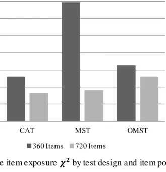
increased constraint complexity. Moreover, CAT and OMST provide higher measurement precision than MST, especially for the large item pool. Finally, CAT is the most secure among the three test designs and the security of MST benefits most from the larger item pool.
TABLE OF CONTENTS
I. INTRODUCTION ... 1
II. LITERATURE REVIEW... 6
Item Response Theory... 6
Dichotomous IRT models. ... 6
Computerized Adaptive Testing... 13
Multistage Testing ... 14
On-the- fly MST. ... 17
Test Specifications ... 17
Item Selection in Adaptive Testing ... 19
Maximum priority index. ... 20
Weighted penalty model. ... 22
MST Module Assembly ... 26 Preassembled MST. ... 26 On-the- fly MST. ... 30 MST by shaping... 31 Research Questions ... 33 III. METHODOLOGY... 35
Item Pool Construction... 35
Test specifications. ... 36
Test Design... 39
MST Preassembly ... 39
Item Response Generation ... 40
CAT simulation. ... 40
Preassembled MST simulation. ... 42
On-the- fly MST simulation. ... 42
Summary. ... 42
Analyses ... 43
Measurement precision. ... 44
Item exposure and test overlap. ... 44
IV. RESULTS ... 46 Content Alignment ... 46 Summary. ... 50 Measurement Precision ... 51 Summary. ... 57 Test Security... 58 Summary. ... 63 V. DISCUSSION ... 64 Content Alignment ... 64 Measurement Precision ... 66 Test Security... 67
Conclusions ... 68
Limitations and Future Directions... 70
REFERENCES ... 73
LIST OF FIGURES
Figure 1. Item Characteristic Curves for three items with varying parameters. ... 7
Figure 2. Item and test information curves for three items with varying parameters. ... 12
Figure 3. Three stage 1-3-3 MST design. ... 15
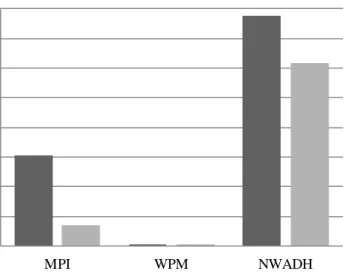
Figure 4. Average number of constraint violations by item selection method and item pool size. ... 48
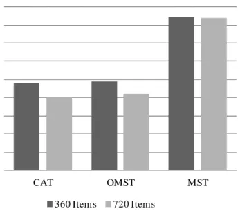
Figure 5. RMSE by test design and item pool size. ... 53
Figure 6. RMSE by test design and test specification complexity. ... 54
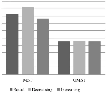
Figure 7. RMSE by test design and stage length. ... 55
Figure 8. Average item exposure by test design and item pool size. ... 59
Figure 9. Average test overlap rate by test design and item pool size. ... 60
Figure 10. Average item exposure by test design and test specification complexity. ... 61
LIST OF TABLES
Table 1 Means, standard deviations, and distributions for item parameter generation ... 36
Table 2 Test blueprint for the baseline content constraint condition ... 36
Table 3 Test blueprint for the simple content constraint condition ... 37
Table 4 Test blueprint for the medium content constraint condition ... 37
Table 5 Test blueprint for the complex content constraint condition ... 37
Table 6 Number of items in each stage across conditions ... 39
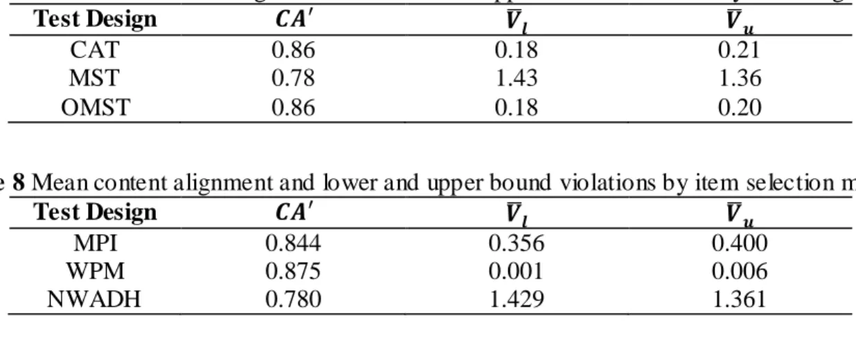
Table 7 Mean content alignment and lower and upper bound violations by test design ... 47
Table 8 Mean content alignment and lower and upper bound violations by item selection method ... 47
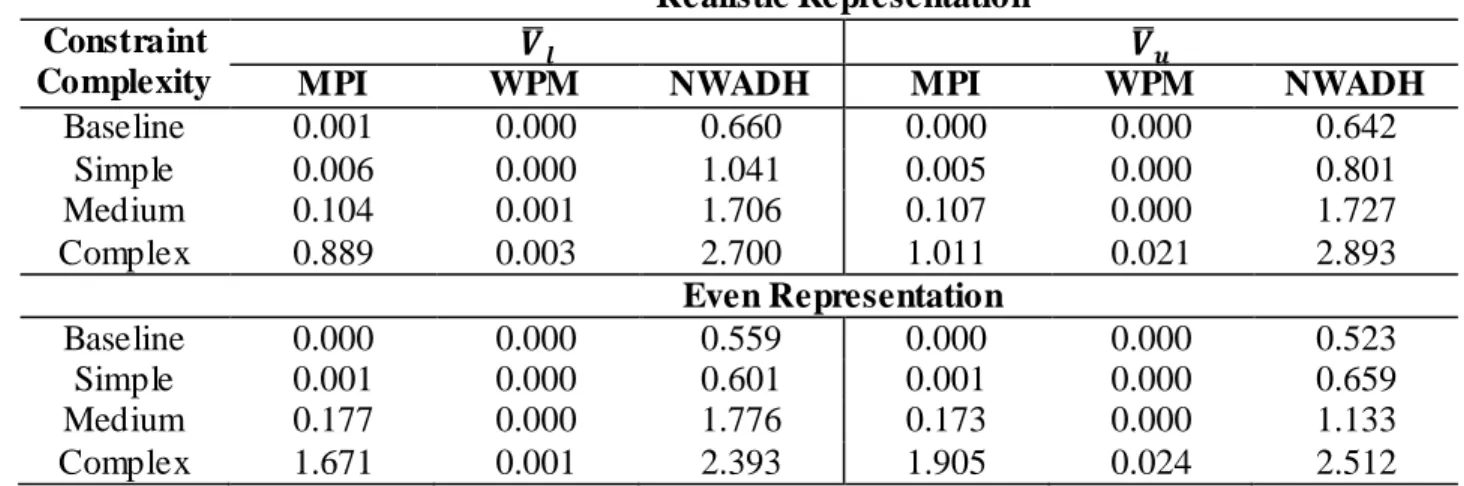
Table 9 Average number of constraint violations by item selection method, constraint complexity, and content representation ... 49
Table 10 Average number of constraint violations by item selection method and stage length .. 50
Table 11 RMSE and bias by test design and item selection method ... 51
Table 12 Average information target by stage and item pool size ... 53
Table 13 Selected and values throughout the test for two average ability examinees ... 56
Table 14 RMSE for the MPI and WPM by test specification complexity... 57
Table 15 Average item exposure , test overlap rate, and proportion of overexposed and unused items by test design ... 58
CHAPTER 1 INTRODUCTION
Over the last several decades, adaptive testing designs, such as computerized adaptive testing (CAT; Lord, 1971b) and multistage testing (MST; Lord, 1971a), have arisen as
mainstream methods for large-scale test administration. These designs adjust the difficulty of the test to the ability of the examinee during test administration. Consequently, compared to the traditional paper-and-pencil linear tests, adaptive tests can provide more precise measurement with fewer items (Stocking, 1994). The traditional CAT is a fully-sequential adaptive design in that items are selected one-at-a-time and ability is estimated after each item. O n the other hand, MST is a group-sequential adaptive design where sets of items, known as modules, are
preassembled at target ability levels and the examinee is routed to the next module based on the ability estimate obtained from responses to the previous module(s).
Both CAT and MST have been successfully implemented in large-scale assessment. Over time, some notable drawbacks of each design have come to light. In CAT, early item responses lead to large changes in estimated ability, as little is initially known about the examinee. Later in the test, changes in estimated ability from one item to the next become smaller. This attribute of CAT makes it difficult for high-ability test takers to recover from early mistakes (Rulison & Loken, 2009). MST is less prone to this issue, as the initial ability estimate is delayed until after a set of items has been completed. As a tradeoff, final ability estimates in MST are often not as precise as those in CAT, as MST modules are designed to be of optimal difficulty only at a limited number of target ability levels (e.g., three levels at low, medium, and high ability). For an examinee whose ability falls between any two target levels (e.g., between low and medium),
difficulty of the modules will not be optimal, and subsequently, ability estimation will not be as accurate as in the CAT design.
To address these issues, researchers have continued to develop new adaptive testing designs. Han and Guo (2014) introduced MST by shaping (MST-S) while Zheng and Chang (2015) proposed “on-the- fly” MST (OMST). Both methods utilize a group-sequential design similar to MST, except that the items are selected during administration, as in CAT. Thus, MST-S and OMMST-ST represent a compromise between CAT and MMST-ST. These new methods still possess many of the advantages of MST but with the additional benefit that final ability estimates can be nearly as precise as CAT. While MST-S and OMST present a promising new direction for adaptive testing, they are relatively new, and more research needs to be done to determine their performance in various testing situations.
Together, CAT, MST, MST-S, and OMST present testing organizations with a myriad of options to achieve precise ability estimation efficiently. However, challenges still exist. For instance, inherent in adaptive testing is a large number of unique test forms. With as many as one unique form per examinee, ensuring that all test forms are equivalent in terms of content can be challenging. Wise, Kingsbury, and Webb (2015) contend that the degree of content alignment for an adaptive test is related to the extent that the test items (1) present an optimal challenge for the examinee, and (2) represent the desired content domain. With respect to the first goal, matching the difficulty of the test to the ability of the examinee is central to adaptive testing. This goal, on its own, can be met in CAT, MST-S, and OMST, and to a somewhat lesser extent in MST. The second goal can be readily accomplished when test forms are created and closely examined before administration, as in linear testing. The challenge in adaptive testing then becomes meeting both goals simultaneously in a test form that is created during administration.
The key to meeting the content alignment standards of adaptive testing lies in the item selection algorithm. Methods that consider item content, in addition to item statistical properties (i.e., information), have been developed for linear testing and preassembled MST (Swanson & Stocking, 1993; Luecht, 1998) as well as CAT (Cheng & Chang, 2009; Shin, Chien, Way, & Swanson, 2009) and OMST (Zheng & Chang, 2015). While these methods have been shown to be effective in many testing situations (He, Diao, & Hauser, 2014), they have not yet been studied for tests with complex content specifications. One example of such constraints comes from the Programme for International Student Assessment (PISA). Its mathematics test uses four indices – content, cognitive process, context, and format type – for each item (OECD, 2012). Each of these categories has 3 or 4 levels and the levels of each category are not exclusive (i.e., items from each content area could be of any cognitive process, context, and format type). Ensuring that each of the levels of each category is adequately represented on every test while also selecting items of optimal difficulty for the examinee can be extremely challenging.
Cheng and Chang (2009) introduced the maximum priority index (MPI) as an item selection method for CAT, which has since been extended to OMST (Zheng & Chang, 2015). The MPI calculates a priority index for each item in the pool based on item content and statistical characteristics. The item with the highest priority index is then selected for administration at each step. The weighted penalty model (WPM; Shin et al., 2009) and normalized weighted absolute deviation heuristic (NWADH; Luecht, 1998) use similar logic to consider both
statistical and non-statistical attributes. The WPM also considers the prevalence of each content area in the item pool in order to account for the quality of the pool while the NWADH aims to assemble multiple test forms that are equivalent in terms of both content and statistical
select items for both linear tests and MSTs. All three methods show potential for assembling tests with very complex content constraints, due to their ability to accommodate situations where items have multiple content indices.
While originally proposed as item selection methods for CAT, the MPI and WPM can be applied to OMST (as in Zheng & Chang, 2015). MST-S, on the other hand, does not use an index to select items; instead, a fixed number of items are randomly s elected from each content area at each stage. This random selection process is repeated a predetermined number of times in order to achieve a desired level of measurement precision and item exposure control. So far, MST-S has only been studied for tests with simple test blueprints (Han & Guo, 2014), as the random nature of MST-S makes it challenging to consider multiple content indices at once.
The main goal of this study is to investigate the effectiveness of item selection methods for adaptive tests with varying levels of test specification complexity. The following five
combinations of item selection method and test design will be studied: MPI and WPM for CAT, NWADH for MST, and MPI and WPM for on-the- fly MST. Evaluation of these methods will be based on the following three criteria: accuracy of ability estimation, satisfaction of test content constraints, and item exposure and test overlap rates. The importance of accurate ability estimation is self-evident. Many score-based decisions depend on the accuracy of latent trait measurement. Satisfaction of test constraints is directly related to the content validity of test scores. Violations of the constraints make the test scores invalid for the target construct and thus difficult to compare across examinees. Item exposure and test overlap rates are test security concerns. Overexposed items and high test overlap rates may result in a testing program that is vulnerable to compromised items due to question sharing between examinees. These three criteria are clearly related and tradeoffs will have to be made among them. For instance,
increasing ability estimation accuracy is likely to co me at the expense of item exposure control, as the best items will be administered more frequently.
The effectiveness of the competing item selection methods may vary by the features of the item pool and test design; hence, these features will be closely examined in this study. Specifically, the size of the item pool, complexity of the test blueprint, representation of each content category in the item pool, number of items in each MST stage, and number of difficulty levels in each preassembled MST stage may all play a role.
CHAPTER 2 LITERATURE REVIEW Item Response Theory
Item Response Theory (IRT) has been the dominant model in large-scale testing since at least the 1970s (Hambleton & Swaminathan, 1985). Different from Classical Test Theory (CTT), which uses number-correct scoring to produce scores that are dependent on the particular set of items included on the test (van der Linden, 1986), IRT focuses on modeling the response probabilities to individual items. Examinee abilities are scored based on the probability of the response pattern instead of the number of correct responses. IRT has many advantages over CTT, such as latent trait estimation that is not dependent on the test and item parameter calibration that is not dependent on the sample.
Dichotomous IRT models. The dichotomous IRT models aim to predict the probability of a correct response to an item. The three-parameter logistic (3PL) model, the most general form, can be expressed as (Birnbaum, in Lord & Novick, 1968):
(1)
The outcome, or , is the conditional probability of a correct response to item
by examinee ( ), given the examinee ability parameter, , and item parameters , ,
and . is a scaling constant used to approximate the normal ogive function by the logistic
function, and is usually set equal to 1.702. The probability of an incorrect response,
or , is simply .
In Equation (1), the item difficulty parameter, , represents the point on the ability ( )
levels and is related to the maximal slope of the item response function. The guessing parameter, , represents the probability of a correct response for an examinee of very low ability (i.e.,
approaching ) (de Ayala, 2009). If , the 3PL model reduces to the two-parameter
logistic (2PL) model. Further nested IRT models are the one-parameter logistic (1PL) model, in
which is restricted to be equal across all items, and the Rasch model, a special case of the 1PL
model where for all items.
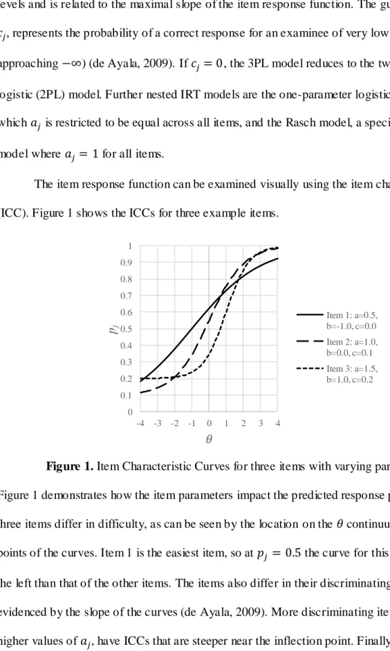
The item response function can be examined visually using the item characteristic curve (ICC). Figure 1 shows the ICCs for three example items.
Figure 1. Item Characteristic Curves for three items with varying parameters.
Figure 1 demonstrates how the item parameters impact the predicted response probabilities. All
three items differ in difficulty, as can be seen by the location on the continuum of the inflection
points of the curves. Item 1 is the easiest item, so at the curve for this item is further to
the left than that of the other items. The items also differ in their discriminating power; this is evidenced by the slope of the curves (de Ayala, 2009). More discriminating items, or items with
higher values of , have ICCs that are steeper near the inflection point. Finally, differences in
0 0.1 0.2 0.3 0.4 0.5 0.6 0.7 0.8 0.9 1 -4 -3 -2 -1 0 1 2 3 4 pj 𝜃 Item 1: a=0.5, b=-1.0, c=0.0 Item 2: a=1.0, b=0.0, c=0.1 Item 3: a=1.5, b=1.0, c=0.2
the guessing parameters can be seen by examining the lower asymptote. The ICC for Item 3 is
nearly flat around , meaning that even very low ability examinees have a nonzero
chance of answering the item correctly by guessing. It should be noted that the presence of a nonzero guessing parameter shifts the entire ICC upward. Thus, the probability of a correct
response at under the 3PL model is not 0.5, but instead can be computed by .
Assumptions. IRT models carry strong assumptions. First, traditional IRT models assume unidimensionality, which states that all items measure only one latent trait. While it might seem impossible for this assumption to be met in practice, due to nuisance factors such as motivation or test-taking skill, this assumption does not need to be met strictly. Generally, it is instead required that there exists one “dominant” trait that accounts for test performance more so than any other trait (Hambleton & Swaminathan, 1985).
The second assumption is local independence, which requires that the response of an examinee to any given test item be independent of all other item responses in the test for any examinee (Birnbaum, in Lord & Novick, 1968). Local independence will be violated when the responses to two or more items are still related after accounting for the target ability. This may occur in situations where several items are related to a common stimulus or responses to later items are made based on responses to earlier items (de Ayala, 2009).
Another important assumption is monotonicity. This assumption requires that the ICC is monotonically increasing and somewhat S-shaped (Hambleton & Swaminathan, 1985).
Monotonicity is important as it demonstrates that the latent trait is being measured by the item(s).
If an examinee has a higher value of , they should have a higher probability of answering the
In general, the form of the ICC should be close to what is specified by the model. The 3PL model thus provides the most relaxed assumptions; items may vary in their difficulty, discrimination, and guessing parameters. For the 2PL model, items may vary in difficulty and discrimination, but should possess a common guessing parameter of 0. Finally, the 1PL and Rasch models have the most stringent assumptions; items must have a guessing parameter of 0 and equal discrimination parameters.
When the above assumptions are met, IRT has the properties of sample- free calibration and test- free measurement. Sample- free calibration means that the values of the item parameters do not depend on the sample of examinees used to calibrate the parameters (Rupp & Zumbo, 2006). Thus, item parameters are invariant across test-takers. The property of test- free measurement indicates that examinee ability estimates do not depend on the particular set of items administered (Hambleton & Swaminathan, 1985). Therefore, unlike in CTT, examinees who respond to different sets of items can still be given comparable scores. These properties are extremely important in adaptive testing, where item parameters are treated as known and
examinees typically see different test forms.
IRT scoring.Ability estimation can be accomplished using maximum likelihood (ML) methods. ML estimation aims to find the model parameters that are most likely to have produced the observed responses. Given local independence, the likelihood of a response pattern is simply the product of the conditional probability of each item response (Hambleton & Swaminathan, 1985):
where is the response to item j and is the Bernoulli distribution for the probability of
an item response. For a correct response, and simplifies to . For an incorrect
response, and becomes .
The probability in Equation (2) is conditional on , meaning each unique value of will
result in a different likelihood for the response pattern. The ML ability estimate is the value of that maximizes the likelihood. One standard method for obtaining the estimate is to set the first
derivative of the log of the likelihood function equal to zero and solve for . As the form of this
derivative is irregular, numerical methods, such as the Newton-Raphson, are often applied (Hambleton & Swaminathan, 1985).
ML estimation can be enhanced by the Bayesian approach that utilizes prior information about the ability distribution in addition to the likelihood function of the response pattern.
Specifically, Bayesian methods multiply the likelihood of the response pattern, given , by the
prior distribution of to obtain the posterior density of . This is expressed as:
(3)
Here is the posterior density of , is the prior distribution, is the marginal
distribution, and is equivalent to in Equation (2). The estimated a
posteriori (EAP) and maximum a posteriori (MAP) estimators, defined as the mean and mode of the posterior distribution, respectively, are commonly used ability estimators in IRT (Hambleton & Swaminathan, 1985).
Bayesian estimation has the distinct advantage of being able to provide an estimate no matter the response pattern. ML estimation will not find a solution if the response pattern is non-mixed (i.e., all 0s or all 1s), as the likelihood function will not have a maximum. A constant
concern with Bayesian estimation, however, is the accuracy of the prior information. In general, research has shown that differences between ML and Bayesian estimates are negligible when items are well- matched to examinee ability, as is the goal in adaptive testing (Wang & Vispoel, 1998; Kim, Moses, & Yoo, 2015).
Information and standard error.Under CTT, measurement accuracy is represented by reliability and the standard error of measurement at the test level. Thus, it is assumed that all examinees are measured to the same degree of accuracy, regardless of ability level. This is rarely true in practice. IRT, on the other hand, provides more localized estimates of measurement error in the form of test information and the standard error of estimate (Embretson, 1996).
Information can be calculated along the continuum at both the item and test levels by
taking the second derivative of the likelihood function with respect to . The formulas for
computing item and test information under the 3PL model, given estimated ability , are given
in Equations (4) and (5), respectively.
(4)
(5)
In Equation (4), item information, , is calculated using the probabilities of a correct and
incorrect response, and , and item parameters and . Equation (5) shows that the test
information, , is simply the sum of item information. Item and test information can also be
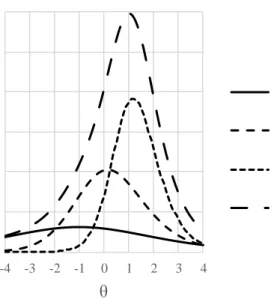
Figure 2. Item and test information curves for three items with varying parameters. Figure 2 clearly shows that item information peaks near the item difficulty parameter while the discrimination parameter determines the amount of information. Guessing introduces noise into the measurement process, thus reducing information (de Ayala, 2009). Accordingly, one way to effectively increase test information is to add items with high discriminating power and difficulty near the examinee’s ability level.
The IRT equivalent of the standard error of measurement is the standard error of
estimate, . Much like the standard error of measurement, represents the uncertainty
associated with the ability estimate and can be used to build confidence intervals for . Equation
(6) shows the relationship between test information and the standard error of estimate (Hambleton & Swaminathan, 1985).
(6)
As is inversely related to test information, the more information that a test provides at ,
the more certain one is about the ability of examinees at . This relationship between
measurement uncertainty and information is critical to item selection in adaptive testing. 0 0.1 0.2 0.3 0.4 0.5 0.6 -4 -3 -2 -1 0 1 2 3 4 Inf or m at ion θ Item 1: a=0.5, b=-1.0, c=0.0 Item 2: a=1.0, b=0.0, c=0.1 Item 3: a=1.5, b=1.0, c=0.2 Test
Computerized Adaptive Testing
Computerized adaptive testing (CAT) aims to select and administer only the most appropriate items for each examinee (Parshall et al., 2002). CAT was originally conceptualized by Lord (1971b) as a method to tailor the test to the examinee by administering items whose difficulties are closely matched to examinee ability. Thanks to increases in computing power, a myriad of options are currently available for CAT administration. Unique design issues, such as the response model, item pool attributes, ability estimation and item selection methods, starting point, and stopping criterion, must be considered when developing a CAT (Weiss & Kingsbury, 1984).
In a CAT administration, items are selected sequentially in a process that can be described in the following steps:
1. Administer the first item from the item pool.
2. Estimate examinee ability based on all item responses.
3. Use the provisional ability estimate to select the best item from the item pool. 4. Administer the item selected in step 3.
5. Repeat steps 2 through 4 until a preset stopping criterion has been reached.
In step 1, the first item can be chosen using the mean of a proposed ability distribution (Mills & Stocking, 1996) or some known information about the examinee (Weiss & Kingsbury, 1984). One can also start the test by simply selecting a relatively easy item to reduce test anxiety (Wainer & Kiely, 1987). Both ML and Bayesian methods can then be used to estimate ability (Wang & Vispoel, 1998). Bayesian methods are typically used at least until a mixed response vector is obtained. In step 3, several algorithms exist for identifying the “best” item.
the item with the highest information at the provisional ability estimate. Algorithms that consider more than just item statistical properties will be discussed in great detail later. Finally, the
stopping criterion can be a fixed number of items, which guarantees an equal test length for all test-takers, an acceptable standard error of estimate, which ensures equal measurement precision for all examinees (Weiss & Kingsubry, 1984), or simply a fixed testing time.
While extremely popular for large-scale testing (Chang, 2015), CAT has received its fair share of criticism. One disadvantage is that ability estimation may be inaccurate at early points in the test, when little information is known about the examinee. These errors in estimation are compounded by the fact that the item selection method depends on the provisional ability estimate. Another downside of CAT is the infeasibility of test form review. In testing, forms are typically reviewed to ensure that test specifications are met and that undesirable characteristics, such as item order or context effects, are not present (Wainer & Kiely, 1987). This is not possible in CAT, as forms are assembled during administration and most examinees will see very
different sets of items, resulting in a large number of unique forms. Finally, examinees are not able to skip items or modify answers to earlier items (Parshall et al., 2002). The issues presented here arise because of the fully-sequential nature of CAT, and can be addressed by a group-sequential adaptive design.
Multistage Testing
Lord (1971a) proposed a two-stage testing design that has since been expanded upon by researchers (e.g., Wainer & Kiely, 1987; Kim & Plake, 1993) and become known as multistage testing (MST). MST adapts in stages, such that ability is estimated only after a set of items has been administered and the next set of items is chosen based on this estimate. In this sense, MST can be considered a compromise between CAT and linear testing, in which all examinees
respond to the same or equivalent test forms. MST utilizes the advantage of tailored testing, adjusting test difficulty to match examinee ability, while also allowing for test form review. These advantages have prompted some testing programs, such as the Graduate Record Examination (GRE), to move completely from CAT to MST (Zheng & Chang, 2014).
In MST, the item sets of differing difficulty levels within each stage are referred to as
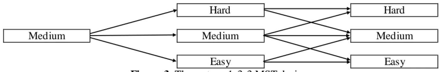
modules. The basic design of an MST can be simply described by the number of stages and the number of modules at each stage. Figure 3 shows a 1-3-3 MST design; that is, a 3-stage MST with one difficulty level in stage 1, and three difficulty levels in both stages 2 and 3.
Stage 1 Stage 2 Stage 3
Hard Hard
Medium Medium Medium
Easy Easy
Figure 3. Three stage 1-3-3 MST design.
Each box in Figure 3 represents a module and the arrows show the possible routes that an examinee can take through the test. Some routes are not permitted; for example, there is no path moving from the hard module in stage 2 to the easy module in stage 3. Such a path would have
indicated an aberrant response pattern. Each route in Figure 3 is called a pathway. Multiple
parallel test forms are usually assembled for each pathway, where each form is called a panel.
Typically, a panel is randomly selected before the first stage (Zheng, Nozawa, Gao, & Chang, 2012). This random assignment helps to ensure even exposure of items in the bank, thus increasing test security. However, since modules at the later stages are chosen based on the provisional ability estimate, examinees of similar ability assigned to the same panel will likely see the same items, increasing the test overlap rate.
MSTs usually begin with a module of medium difficulty, as shown in Figure 3 (stage 1).
After the first module, also known as a routing test, examinees are assigned to the next module
using either number-correct or IRT scoring (Weissman, Belov, & Armstrong, 2007). Typically, routing is accomplished by setting cut points, either by finding the point where the two adjacent module information curves cross (e.g., Zheng et al., 2012) or by using assumptions about the ability distribution to route a certain percentage of examinees to each module (e.g., Jodoin, Zenisky, & Hambleton, 2006). Using the crossing point of the module information curves often results in more precise measurement, as this is akin to choosing the most informative module for the examinee, while routing based on the ability distribution allows for better test security, as
each module can be exposed to a set proportion of examinees. Examinees with (or
number-correct score) below the first cut point, , are routed to the easiest module while examinees with
receive the second easiest module, and so on.
MST presents many advantages over both CAT and linear testing. Compared to CAT, provisional ability estimates are more accurate at early stages, as more items are administered between each estimation point. Second, MST forms can be preassembled and each possible pathway can be carefully reviewed with context and item order effects in mind (Wainer & Kiely, 1987). Third, the MST design allows examinees to skip and review items within a stage (Zheng et al., 2012). Finally, since MST is still adaptive, it provides more precise ability estimation than linear testing. Compared to CAT, one obvious disadvantage of MST lies in having fewer
adaptation points. While CAT adapts after each item, MST adapts only after each stage. Also, as
each module maximizes information at only one point, examinees whose abilities are far from
the target abilities will receive modules that are not of ideal difficulty. This mismatch reduces the accuracy of final ability estimation.
On-the-fly MST. Two methods have been proposed to increase the measurement
precision of MST: MST by shaping (MST-S; Han & Guo, 2014) and “on-the- fly” MST (OMST; Zheng & Chang, 2015). Like MST, MST-S and OMST are administered in stages and examinee ability is estimated only after the completion of each stage. However, in MST-S and OMST, there are no panels, no preassembled modules at fixed difficulty levels, and no routing rules. Instead, items within each stage are chosen during administration, based on the provisional ability estimate. MST-S accomplishes this by randomly selecting items iteratively for inclusion in the next stage. The set of items that minimizes the distance from the target information value is then chosen for administration. OMST, on the other hand, utilizes sequential item selection methods developed for CAT to build MST stages on-the- fly. Both methods have been shown to result in measurement precision close to that of CAT and considerably better than MST (Han & Guo, 2014; Zheng & Chang, 2015).
Test Specifications
Over the last two decades, educational policy, such as No Child Left Behind and Every Student Succeeds, has focused on holding schools accountable via assessments that are aligned to certain content standards. This alignment between educational standards and test content is critical to ensuring that inferences made from test scores are valid. Webb (2006) described four criteria that can be used to judge the alignment of an assessment. Categorical concurrence describes the degree to which topics or categories (e.g., algebra, geometry) within the broader category (e.g., mathematics) are represented both in the standards and on the test. Depth-of-knowledge relates to the cognitive demand, or complexity, of what students are required to do. Finally, range-of-knowledge and balance of representation refer to the span of knowledge required and the distribution of topics on the test, respectively. As they relate to the test content
specifications, the first two criteria describe what levels of content and complexity are to be assessed while the last two criteria define the distribution of these levels across the test.
Evaluation of these criteria are based on judgments made by subject matter experts and are not the same as item statistical properties, which are usually based on the actual testing data.
Content specifications are one aspect of the overall test specifications, which may also include item format, context, or other traits important to the goal of measurement (Webb, 2006). The complexity of test specifications can vary greatly by assessment. For example, the test blueprint for the National Assessment of Educational Progress (NAEP) reading assessment includes two levels of passage type and three levels of cognitive targets (National Assessment Governing Board, 2015b). In comparison, the NAEP mathematics assessment specifies five levels of item content, three levels of cognitive complexity, and two levels of item format (National Assessment Governing Board, 2015a). Thus, the specifications for the mathematics assessment are much more complex than that of the reading assessment, even within the same testing program.
In adaptive tests, content alignment is defined by the agreement between the ability of the examinee and the difficulty of the test form, as well as the representation of the desired content domain (Wise et al., 2015). While the adaptive designs outlined previously were created with the intention of tailoring the test difficulty to match examinee ability, representation of the content domain is not inherent in these designs. That is to say, features like categorical concurrence, depth-of-knowledge, and balance of representation are not explicitly addressed. Additionally, further test specifications, such as item context or format, are also not a utomatically controlled by the test design. If test forms are to be created during administration, the item selection
algorithm will need to ensure that each test is aligned to the content standards and other criteria expressed by the test blueprint.
Item Selection in Adaptive Testing
The item selection algorithm arguably plays the most important role in adaptive testing. This algorithm must balance three elements: measurement precision, test specifications, and item exposure. Unfortunately, these often work against one another. For instance, high measurement precision requires selecting highly informative items, but repeated selection of those items will lead to their overexposure. Additionally, ignoring content specifications may result in tests that differ in content validity (Mills & Stocking, 1996; Wise et al., 2015). Thus, the goal of the item selection algorithm is threefold: to achieve maximum measurement precision, to satisfy test specifications, and to reduce item overexposure and test over lap.
In early versions of adaptive testing, item selection focused only on item information while content balancing was seen as a fairly simple problem. Kingsbury and Zara (1989)
described a mathematics test where addition and subtraction problems were required to make up 30% of the test each while the remaining 40% was divided equally between multiplication and division items. The authors’ proposed solution was simply to select the maximally informative item from the content category that was furthest from meeting its desired percentage. However, as outlined previously, test blueprints often categorize items by more than just the content area. When more than one categorical label is assigned to each item, the simple methods proposed in early CAT studies (e.g., Kingsbury & Zara, 1989) will not suffice.
Item selection in tests with many constraints is typically accomplished using one of two methods: 0-1 linear programming and heuristics. Linear programming methods attempt to maximize information across the test, subject to the test constraints; constructing the entire test
form at once. The shadow test approach (van der Linden & Reese, 1998) is an example of a 0-1 linear programming approach that can be applied to adaptive testing. Heuristic methods, on the other hand, build the test one- item-at-a-time by treating test construction as a series of local optimization problems (Zheng & Chang, 2014). Unlike linear programming methods, heuristics do not attempt to find a perfect solution, but they are generally faster, computationally simpler, and will at the very least minimize constraint violations. When the test blueprint is complex, heuristics can be very useful, as linear programming methods may e ncounter infeasibility issues, where no test is created because no perfect solution can be found (Cheng & Chang, 2009). Accordingly, this study focuses on heuristic methods.
Maximum priority index. The maximum priority index (Cheng & Chang, 2009) combines the statistical and non-statistical attributes of test items by multiplying item
information by a value that measures the item’s contribution toward meeting the test constraints.
The item that maximizes this product is chosen for administration. The priority index for item ,
, given the provisional ability estimate , can be calculated as:
(7)
Here, each constraint is represented by and is dummy coded such that is 1 when constraint
is relevant for item and 0 otherwise. The weights, , are part of the test blueprint and are
assigned based on the importance of each constraint, with larger weights associated with major
content areas. Finally, for each constraint, measures the proportion of the constraint that still
needs to be met. This is calculated by:
(8)
where represents the number of items required from constraint category and is the
Oftentimes, the test blueprint will specify a lower ( ) and upper ( ) bound for each constraint. These bounds represent the minimum and maximum number of items allowed from
category . In these cases, the MPI requires a two-phase selection procedure, where phase one
focuses on meeting the lower bounds and phase two tries not to exceed the upper bounds. In
phase one, items may be selected from content area until , or . Once all content
areas have satisfied their lower bounds (all ), phase one ends. In phase two, items can be
selected from content area until . The two-phase MPI ensures that all lower bounds
will be met as long as the test length is sufficient and upper bounds will not be exceeded unless the test is too long (Cheng & Chang, 2009).
The MPI presents several options for controlling item exposure. Cheng and Chang (2009)
suggested specifying a desired exposure rate as a constraint. To do this, in Equation (8) is
replaced by the desired exposure rate and is updated to represent the current exposure rate,
which is the number of times item has been administered divided by the total number of tests.
Items with current exposure rates higher than the desired rate will have negative values of ,
making them unlikely to be selected. He et al. (2014) applied a randomesque method similar to that of McBride and Martin (1983) in which the administered item is chosen randomly from a
group of items with the highest . All items in the group, including the unselected items, are
then eliminated from the pool for the remainder of the test. Introducing randomness into the selection process ensures that the “best” item is not selected every time, reducing the chance of item overexposure.
The MPI is a very straightforward item selection method that considers all three aspects of item selection. Measurement precision is addressed through the presence of item information, deviations from the content constraints consider the test specifications, and exposure control can
be incorporated as outlined above. Cheng and Chang (2009) likened the MPI to a simple modification of the maximum information method that instead considers the overall
“attractiveness” of the item in terms of both statistical and non-statistical properties. The content
weights, , can be adjusted to control the scale of the priority index. That is, larger weights can
be used if test specifications are deemed to be more important than item information.
Weighted penalty model. Similar to the MPI, the weighted penalty model (Shin et al., 2009) assigns a unique penalty value to each item at each selection point. The item with the
smallest penalty value is then selected for administration. The penalty value for item , , is
calculated as:
(9)
where and represent the standardized penalty values for item content and information,
respectively. The weights associated with content and information, and , control the
trade-off between non-statistical and statistical item properties and can be updated throughout the test. Shin et al. suggested changing the information weight throughout the test based on a logistic or quadratic function so that item selection focuses on meeting test constraints early in the test before giving larger weight to information near the end.
The constraint penalty value, , is computed in five steps. The first step is to compute
, the proportion of items from category that would be administered by the end of the test if
items from were selected in proportion to their prevalence in the remaining item pool. This can
be written as:
Here, and are the number of items administered so far and the number of items administered
from constraint category so far, respectively. The prevalence, , is the proportion of items
from in the complete item pool and is the test length (Shin et al., 2009).
Next, the difference between the projected proportion of items to be administered from and the midpoint of the lower and upper bounds is calculated by:
(11)
where is the midpoint between the lower and upper bounds. For the WPM, the lower and
upper bounds, and , are expressed as proportions; thus, represents the midpoint between
the lowest and highest acceptable proportion of test items from category . The deviation from
the midpoint, , is then used in one of Equations (12) through (14) to calculate , the penalty
value specific to category .
If then (12) If then (13) If then (14)
Shin, Chien, and Way (2012) defined as the quadratic distance between the number of items
administered from so far and the midpoint of the lower and upper bounds of . It can be seen
that when , will be lower, as is always negative. On the other hand,
categories with will have positive values of . Thus, penalty values are lower for items
from categories that may not meet their lower bounds and higher for items from categories that may exceed their upper bounds.
In the third step, the total content penalty value for item is calculated using the
content-specific penalties and weights, and , respectively, and the dummy code for item belonging
to category , :
(15)
Here, is the unstandardized content penalty value and consists of the product of the content
penalty value and its associated weight, summed across all content categories relevant to item .
The weights, , are defined by the test blueprint, as in the MPI (Equation (7)). The final step for
computing is to standardize the penalty value using the minimum ( ) and maximum
( ) content penalty values across all items remaining in the pool (Shin et al., 2009):
(16)
Similarly, the standardized information penalty value, , is calculated using the
information at for item and the maximum information at across all items remaining in the
pool, :
(17)
Note that the standardized information value is multiplied by negative one. Thus, items with more information will have smaller (negative with larger absolute value) penalty values, making
them more likely to be selected (Shin et al., 2009). After computing and , these values are
substituted into Equation (9) to determine . The item that minimizes is chosen for
administration.
The techniques used to control item exposure with the WPM are similar to those applied to the MPI. Shin et al. (2009) recommended using a conditional randomesque procedure where
estimate. Conditioning the item selection group size on ability, as proposed by Kingsbury and Zara (1989), accounts for the fact that the item pool may have more items available at some difficulty levels than others. An unconditional randomesque procedure (i.e., McBride & Martin, 1983) can also be used, or the desired exposure rate could be specified as a constraint, as
recommended for the MPI by Cheng and Chang (2009).
The WPM is not as a simple and straightforward as the MPI. There are, however, some notable advantages to this method. First, the WPM uses the prevalence of the content area in the item pool to project the number of items that will be administered. It is this projection, rather than the current deviation from the bounds, that determines which items will be given more preference. This helps account for any differences in the representation of each content category
in the item pool. Second, since the WPM uses the quadratic distance from the midpoint ( in
Equations (12) and (13)), a relatively larger penalty is assigned to items that violate content constraints and more preference is given to items that do not (Shin et al. 2012). Finally, the WPM standardizes both the content and information penalty values. Thus, these values are on a
similar scale and the content and information weights, and , can more readily be
manipulated to control the tradeoff between statistical and non-statistical attributes.
Both the MPI and WPM have performed well in CATs with simple constraints. They are capable of meeting test specifications and minimizing item overexposure with minimal sacrifices in measurement precision. He et al. (2014) showed that the WPM was able to meet constraints more consistently than the MPI. The two methods did not differ in measurement precision or exposure control. Computationally, the MPI is much simpler than the WPM. However, the WPM possesses many theoretical advantages over the MPI, as discussed above.
MST Module Assembly
The group-sequential nature of MST lends itself to several options for module assembly. Preassembly of MST forms allows for each module and pathway to be reviewed by content area experts and test specialists at the possible expense of measurement precision, as items may not be of optimal difficulty for all examinees. O n-the-fly assembly, on the other hand, prioritizes measurement precision over test form review and thus relies more heavily on the item selection algorithm. Item selection methods for both preassembled and on-the- fly assembled MST are discussed next.
Preassembled MST. When modules are preassembled, MST design aspects, such as the number of stages, the number of difficulty levels within each stage, and the number of parallel panels, will greatly impact measurement precision and item exposure rates. In general, greater precision can be achieved by including more stages, or adaptation points. Designs with more than two stages are recommended, as this gives the test an opportunity to recover from any inappropriate routings that may occur after the initial stage (Zheng & Chang, 2014).
Measurement precision can be greatly impacted by the number of difficulty levels within each stage. Research has shown that a maximum of four difficulty levels at the final stage is desired while three difficulty levels will usually suffice (Armstrong, Jones, Koppel, & Pashley, 2004). Aspects such as the number of items included in each stage can also impact measurement precision. Longer routing tests achieve more accurate routing with the tradeoff of decreased precision by including fewer items in later stages when more is known about the examinee (Kim & Plake, 1993). Finally, it can easily be seen that the number of stages, difficulty levels in each stage, and panels will all impact item exposure and test overlap rates; more stages, difficulty levels, and panels will lead to lower item exposure and test overlap. These features of the MST,
which need to be decided on before assembling the test forms, can be just as important as the item selection method.
Once the details of the MST design have been established, the test assembly method has three goals: (1) to make the information functions of different modules within a stage distinct enough to provide appropriate adaptation; (2) to make the information functions of
corresponding pathways similar across all panels; and (3) to meet all test specifications in every pathway and panel (Zheng, Wang, Culbertson, & Chang, 2014). The first two goals concern the target information function (TIF) of the modules and panels, respectively, while the third goal
considers the test blueprint. These goals can be met using either a bottom-up or top-down
approach (Luecht & Nungester, 1998). In the bottom- up approach, module- level TIFs and constraints are specified and each module is assembled individually to meet these criteria. Thus, any combination of modules should result in a pathway that meets the test-wide TIF and content constraints. Top-down assembly, on the other hand, focuses only on test-wide TIFs and
constraints and attempts to meet these criteria in each pathway and panel. While top-down assembly may be easier when constraints are specified at the test level, bottom- up assembly allows for modules to be mixed and matched, resulting in lower test overlap rates. Since heuristic item selection approaches focus on local optimization, these methods often utilize a bottom- up strategy (Zheng et al., 2012).
Normalized weighted absolute deviation heuristic. While the MPI and the WPM have not been applied to MST preassembly, the normalized weighted absolute deviation heuristic (Luecht, 1998), a similar method, has been used successfully (Zheng et al., 2012). The NWADH can be used to select items one-at-a-time for inclusion in a stage (Zheng & Chang, 2015). The
(18)
where is the normalized weighted absolute deviation. The normalized absolute deviation from
the TIF is represented by while each represents the normalized absolute deviation from
constraint . Once again, is a dummy code representing whether or not item belongs to .
The weights, and , are specified for the TIF and each content constraint, respectively
(Luecht, 1998).
At each selection point, the normalized absolute deviation from the TIF is calculated for every item remaining in the pool as:
(19)
where represents all items in the pool except for the items already included on the
test. The are computed as:
(20)
where represents the target test information at . Subtracted from is the sum of the item
information at for the items included on the test so far. The denominator is the number
of items remaining on the test, where is the total test length. Thus, represents the absolute
deviation for item from the average information required over the remaining test items (Luecht,
1998).
To compute , the normalized absolute deviation from constraint , Luecht (1998)
suggested assigning weights to each constraint, , such that:
if then (21)
if then (22)
Note that these weights are not the same as the used in Equation (18). Items that have not yet met their lower bounds will be given more weight than those that have and items that have met
their upper bounds will be given no weight. A complement to , Wc, is then computed as:
Wc (24)
where is the maximum out of the constraints. Finally, the used in Equation
(18) are calculated by first finding :
Wc (25)
then normalizing to by:
(26)
The NWADH is similar to the MPI and the WPM in that item information and deviations from the content constraints are combined into one index. The differences between the NWADH and the other two heuristics reflect the differences between the goals of CAT item selection and those of MST assembly. First, rather than focusing on information at a provisional estimate, the
NWADH computes information at predetermined target s. This allows for adaptation in the
preassembled test form. Second, the NWADH aims to minimize deviations from the target information function instead of simply maximizing information. This needs to be done to ensure that all modules within a stage and across panels have similar information functions. Finally, when the bottom- up assembly approach is used, the NWADH focuses on meeting content constraints at the module level, rather than across the entire test. Meeting constraints within each module helps to ensure that each pathway meets the test constraints.
The NWADH has been successfully applied to both linear (Luecht, 1998) and MST (Zheng et al., 2012; Zheng & Chang, 2015) assembly. Both MST studies used bottom-up
assembly. Zheng et al. (2012) found that backward assembly of MST modules, where later modules are assembled first, led to higher classification accuracy compared to forward assembly. This was attributed to the fact that the later stages are more complex, in that there are more modules of differing difficulty levels. Assembling these modules may require access to the full item pool. If assembled later, when the pool has shrunk considerably, estimation accuracy may suffer. Zheng and Chang (2015) found that MSTs assembled using the NWADH led to lower measurement precision than CAT and OMST with item selection via the MPI. This, however, is likely an effect of differences in the test design, rather than a deficiency in the test assembly heuristic.
On-the-fly MST. When MST stages are built on-the- fly, CAT item selection methods can be used to choose items for each stage. Zheng and Chang (2015) demonstrated this with the MPI. In their method, items are added to each stage one-at-a-time. Thus, the formulas are the same as those outlined in Equations (8) and (9); however, item information only needs to be calculated once for each item at each stage, since the entire stage is based o n the same
provisional ability estimate. The content constraint deviations ( ), on the other hand, must be
updated after each selection, due to the change in the number of items administered from the content area(s).
After a stage of items is selected, an item replacement step can be added where test specifications for the stage are evaluated and items are replaced as needed. Zheng and Chang (2015) outlined the steps for item replacement when a lower bound violation exists for the stage-specific content constraints. These steps are as follows:
1. For every lower bound violation of constraint , identify a constraint that is above its
2. Replace a randomly selected item from in the current set with the item from with
maximum information at in the item pool.
3. Evaluate the constraints for the current set of items and repeat steps 1 and 2 until a set has
been found that meets all constraints.
By utilizing an item replacement step, it is guaranteed that every test will meet the constraints, provided that meeting all constraints is possible given the test or stage length, test blueprint, and item pool characteristics. Zheng and Chang reported zero constraint violations in their study, but their test specifications were very simple and the authors did not report how often the item replacement step was needed.
The MPI has been shown to result in similar measurement precision when applied to OMST, compared to CAT, while also minimizing constraint violations (Zheng & Chang, 2015). Research on OMST, however, has been limited to tests with very simple constraints. Zheng and Chang’s (2015) study only required that one item be administered per stage from each of eight content areas. As each stage included 15 items, these constraints could be met fairly easily. It is not clear how item selection will work when each item belongs to several categories that must be constrained. Additionally, situations where constraints are specified only at the test level, where the number of constraints may exceed the number of items in each stage, have yet to be
discussed. Finally, other heuristic item selection methods, such as the WPM, have not yet been applied to OMST.
MST by shaping. Han and Guo (2014) proposed MST by shaping, a different method for assembling MST stages during administration. This method aims to create stages that will help meet the test specifications and TIF. Specifically, after a stage of items has been completed, the provisional ability estimate and current test information at this estimate are calculated. Next, the
difference between the current information and the TIF is used to develop a TIF mold, which represents the ideal information function for the next stage. In the item selection step, the number of items required from each category is determined from the test specifications and items are randomly selected in accordance with these constraints.
After the initial set of items is selected, the difference between the information function for the current set of selected items and the TIF mold is calculated as:
(27)
Here, is the information at for the currently selected items and is the information at
for the TIF mold for stage . After calculating for the current set, the first item in the set is
replaced with another random selection from the same content area and is recalculated. If the
new item leads to a decrease in , this item is kept in the stage. If not, the new item is discarded
from the pool for the current stage and the initial item is kept in the stage. This random item replacement is repeated for each item in the stage, and then the entire process is repeated for a fixed number of iterations. The set of items that comprises the stage after the final iteration is then administered to the examinee (Han & Guo, 2014).
MST-S attempts to meet test constraints by selecting the appropriate number of items from each content area in each stage. The tradeoff between measurement precision and item exposure is controlled by the number of iterations in the item selection, or shaping, process. For example, if the item selection process does not iterate, the resulting test will be a random set of items from each content area. Thus, measurement precision will be poor but item exposure will be ideal. On the other hand, if the number of iterations is 100, the resulting stages will likely feature items of near optimal difficulty for the examinee. However, the randomness of the
selection process will be greatly reduced and items with high (i.e., high information) may be selected too frequently.
Results of Han and Guo’s (2014) initial study on MST-S are promising. When the shaping process iterated only three times, the standard error of the resulting ability estimates were comparable to those in a preassembled MST. As the number of iterations increased, results approached the precision levels of CAT. In terms of item exposure, MST-S had more even exposure rates than both preassembled MST and CAT when up to six iterations were used in the shaping process. Predictably, as the number of iterations increased to 100, items with high became overexposed. This overexposure, however, was still not as extreme as in CAT with maximum information item selection. MST-S is still very new; Han and Guo’s study is the lone demonstration of this method. While this method is ideal for controlling the tradeoff between measurement precision and item exposure, MST-S can only be applied to tests with simple content constraints. When items are classified on more than one variable, the random selection required by MST-S does not allow for the consideration of multiple indices for each item. Thus, this method will not be examined in this study.
Research Questions
The main purpose of this study is to evaluate the performance of heuristic item selection methods on adaptive tests with various levels of test specification complexity. Specifically, the following research questions are of interest:
1. How does on-the- fly MST compare to preassembled MST and CAT on tests with
complex constraints?
2. How do the different heuristic item selection methods compare within and between
The test designs to be compared will be: CAT with MPI item selection, CAT with WPM item selection, MST preassembled with the NWADH, OMST with MPI item selection, and OMST with WPM item selection.
CHAPTER 3 METHODOLOGY
A Monte Carlo simulation study was conducted to evaluate the effectiveness of the aforementioned item selection methods and adaptive testing designs. Complexity of the test specifications, representation of each content category, item pool size, the number of items in each stage, and number of difficulty levels in the preassembled MSTs were varied to simulate typical testing conditions. The outcomes of interest were alignment with test specifications, measurement precision, and item exposure and test overlap rates.
The simulation began by randomly generating examinee abilities, item parameters, and item content categorizations. Next, MST forms were preassembled from the item pool.
Responses were then generated for each examinee on each of the testing designs. Each test contained 36 items. Final ability estimates were recorded, along with the items administered on each test and their corresponding content categorizations. This information was used to calculate root mean square error (RMSE) and bias for ability estimation, the number and type of constraint violations, a general index of content alignment, and item exposure and test overlap rates. Item Pool Construction
Previous MST studies have typically used a fixed item pool of moderate size, ranging from 420 to 600 items (Routo, Patsula, Manfred, & Riza vi, 2003; Zheng et al., 2012; Han & Guo, 2014). In this study, the item pool size was varied at two levels – 360 and 720 items – to represent a small and large pool. To make the item pools realistic, item parameters were
generated using real item pools. As described in Table 1, the means and standard deviations were based on the pool used in Zheng et al. (2012) while the distributions followed Edwards, Flora, and Thissen (2012). In both studies, the item parameters came from operational tests.
Table 1 Means, standard deviations, and distributions for item parameter generation
Parameter Mean Standard Deviation Distribution
1.196 0.329 Lognormal
0.060 1.430 Normal
0.153 0.072 Logit-normal
For the and parameters, the means listed in Table 1 represent the means of the parameters
after transforming to the appropriate distribution. Compared to the mean of 1 and standard
deviation of 0.5 often used in simulation studies, the parameters used in this study are larger
and more centered. In other words, the items are better. This is due to the fact that adaptive tests
are very dependent on the quality of the items. The same case can be argued for the parameter
distribution. Similar to most IRT simulation studies, the parameter distribution has a mean
close to 0, but the standard deviation in this study is larger than 1. This distribution has a wide
spread in order to better cover the entire distribution. Examinee abilities were generated from a
standard normal distribution. Sample size was set at 1,000. This size and distribution are similar to those used in Kim, Chung, Dodd, and Park (2012) and Zheng et al. (2012).
Test specifications.Test specification complexity was based on real large-scale test blueprints. The complexity of the test specifications can be summarized by the number of indices associated with each item. Each item is characterized by one, two, three, or four categories for the baseline, simple, medium, and complex specifications, respectively. The baseline condition was based on the blueprint described by Kingsbury and Zara (1989) and is shown in Table 2.
Table 2 Test blueprint for the baseline content constraint condition
Constraint Category Level % of ite ms in pool
Content
Addition 30%
Subtraction 30%
Multiplication 20%
The simple blueprint, shown in Table 3, simulates the one used for the NAEP 12th grade reading test (National Assessment Governing Board, 2015b).
Table 3 Test blueprint for the simple content constraint condition
Constraint Category Level % of ite ms in pool
Passage type Literary 30%
Informational 70%
Cognitive targets
Locate/recall 20%
Integrate/interpret 45%
Critique/evaluate 35%
The medium complexity blueprint simulates the one used in the NAEP 12th grade mathematics
test (National Assessment Governing Board, 2015a). This blueprint is shown in Table 4. Table 4 Test blueprint for the medium content constraint condition
Constraint Category Level % of ite ms in pool
Content
Number properties and operations 10%
Measurement 15%
Geometry 15%
Data analyses, statistics, and probability 25%
Algebra 35%
Complexity
Low 25%
Moderate 50%
High 25%
Format Multiple choice 50%
Constructed response 50%
Table 5 shows the most complex test blueprint condition. These specifications are akin to those used in the PISA mathematics assessment (OECD, 2012).
Table 5 Test blueprint for the complex content constraint condition
Constraint Category Level % of ite ms in pool
Content
Change and relationships 27%
Quantity 26%
Space and shape 24%
Uncertainty and data 23%
Cognitive process Formulate 25% Employ 44% Interpret 31% Context Occupational 23% Personal 29% Public 25%