Henrik Nyman
Context-Specific Independence
in Graphical Models
H
en
rik
N
ym
an
| C
on
te
xt-Sp
ec
ifi
c In
de
pe
nd
en
ce
in
G
ra
ph
ica
l M
od
els
| 2
01
4
Context-Specific Independence
in Graphical Models
Henrik Nyman
Mathematics and Statistics Department of Natural Sciences
Supervisor
Professor Jukka Corander, University of Helsinki, Helsinki
Reviewers
Associate Professor Jose M. Pe˜na, Link¨oping University,
Link¨oping
Professor Emeritus Stefan Arnborg, Royal Institute of Technology, Stockholm
Opponent
Professor Emeritus Stefan Arnborg, Royal Institute of Technology, Stockholm
Preface
This thesis represents the end product of the research I have done at ˚Abo Akademi University during the years 2010 - 2014. During this time I have learned a lot, not only what it means to be a researcher, but as a person as well. Although I have put a lot of time and effort into this thesis I could by no means have done it by myself and much of the credit should go to the people who have supported me in one way or another.
First and foremost I would like to thank my supervisor Jukka Corander. It will never cease to amaze me how one man can work on so many projects at once while still being in complete control of each one. Although we have worked in different cities I have always been able to count on Jukka answering e-mails, both regarding pressing issues and in some cases maybe not so pressing issues, at a moment’s notice.
A very special thanks goes to my closest colleague Johan Pensar. It is safe to say that my work on this thesis only first really came alive when he joined team BAPS ˚Abo division, doubling the number of members of our proud society. When thanking Jukka and Johan it is impossible not to mention mister Moretti and everybody at Hotel Cepina, the site of summer permafrost 2012-2014, where a large part of the ideas culminating in this thesis were hatched.
I would also like to thank everybody at the mathematics and statistics de-partment. Especially G¨oran H¨ogn¨as and Paavo Salminen for helping with all kinds of practical and financial matters. The amount of help I have received during the years from fellow PhD students, Paul, Brita, Mikael, and many other students past and present has also been invaluable. For their financial support I would like to thank the Center of Excellence in Optimization and Systems Engineering at ˚Abo Akademi University and the Foundation of ˚Abo Akademi University.
Of course a big thanks also goes to the other co-authors of the articles included in this thesis, Timo Koski and Jie Xiong. As well as to Jose M. Pe˜na for agreeing to review this thesis and Stefan Arnborg, both for reviewing the thesis and acting as opponent.
Last, but definitely not least, a huge thanks goes to my family and friends for all the support they have given me through the years. I cannot ever thank my parents enough for everything they have done for me. I would not be half the person I am today without your love and guidance. And of course, Sara my guiding light whose support I can always rely on in the good times, and more importantly, in adversity.
Abstract
The theme of this thesis is context-specific independence in graphical models. Considering a system of stochastic variables it is often the case that the variables are dependent of each other. This can, for instance, be seen by measuring the covariance between a pair of variables. Using graphical models, it is possible to visualize the dependence structure found in a set of stochastic variables. Using ordinary graphical models, such as Markov networks, Bayesian networks, and Gaussian graphical models, the type of dependencies that can be modeled is limited to marginal and conditional (in)dependencies. The models introduced in this thesis enable the graphical representation of context-specific independen-cies, i.e. conditional independencies that hold only in a subset of the outcome space of the conditioning variables.
In the articles included in this thesis, we introduce several types of graphi-cal models that can represent context-specific independencies. Models for both discrete variables and continuous variables are considered. A wide range of properties are examined for the introduced models, including identifiability, robustness, scoring, and optimization. In one article, a predictive classifier which utilizes context-specific independence models is introduced. This classi-fier clearly demonstrates the potential benefits of the introduced models. The purpose of the material included in the thesis prior to the articles is to provide the basic theory needed to understand the articles.
Sammanfattning
Temat f¨or den h¨ar avhandlingen ¨ar kontextspecifikt oberoende i grafiska mod-eller. F¨or en m¨angd stokastiska variabler g¨aller det i regel att variablerna ¨ar beroende av varandra. Graden av beroende kan t.ex. m¨atas med kovariansen mellan tv˚a variabler. Med hj¨alp av grafiska modeller ¨ar det m¨ojligt att visualis-era beroendestrukturen f¨or ett system av stokastiska variabler. Med hj¨alp av traditionella grafiska modeller s˚asom Markov n¨atverk, Bayesianska n¨atverk och Gaussiska grafiska modeller ¨ar det m¨ojligt att visualisera marginellt och betingat (o)beroende. De modeller som introduceras i denna avhandling m¨ojligg¨or en grafisk representation av kontextspecifikt oberoende, d.v.s. betingat oberoende som endast h˚aller i en delm¨angd av de betingande variablernas utfallsrum.
I artiklarna som inkluderats i denna avhandling introduceras flera typer av grafiska modeller som kan representera kontextspecifika oberoende. B˚ade diskreta och kontinuerliga system behandlas. F¨or dessa modeller unders¨oks m˚anga egenskaper inklusive identifierbarhet, stabilitet, modellj¨amf¨orelse och optimering. I en artikel introduceras en prediktiv klassificerare som utnyttjar kontextspecifikt oberoende i grafiska modeller. Denna klassificerare visar tydligt hur anv¨andningen av kontextspecifika oberoende kan leda till f¨orb¨attrade resul-tat i praktiska till¨ampningar. M˚alet med materialet som presenteras i avhan-dlingen ut¨over artiklarna ¨ar att ge de grundkunskaper som beh¨ovs f¨or att f¨orst˚a inneh˚allet i artiklarna.
Contents
Preface iii
Abstract iv
Sammanfattning iv
Contents v
List of original articles vi
Authors’ contributions to Articles I-V . . . vi
1 Introduction 1
2 Graphical models 3
2.1 Markov networks and Bayesian networks . . . 3 2.2 Gaussian graphical models . . . 5
3 Context-specific independence 6
4 Using Markov chain Monte Carlo methods to perform model
optimization 8
4.1 Markov chains . . . 8 4.2 Markov chain Monte Carlo methods . . . 9
5 Classification 12
6 Summaries and discussion of Articles I-V 14
6.1 Article I: Stratified graphical models - context-specific indepen-dence in graphical models . . . 14 6.2 Article II: Labeled directed acyclic graphs: a generalization of
context-specific independence in directed graphical models . . . . 14 6.3 Article III: Context-specific independence in graphical log-linear
models . . . 15 6.4 Article IV: Stratified Gaussian graphical models . . . 16 6.5 Article V: Marginal and simultaneous classification using
strati-fied graphical models . . . 17
List of original articles
I Nyman, H., Pensar, J., Koski, T., & Corander, J. (2014). Stratified graph-ical models - context-specific independence in graphgraph-ical models. Bayesian Analysis. doi:10.1214/14-BA882.
II Pensar, J., Nyman, H., Koski, T., & Corander, J. (2014). Labeled di-rected acyclic graphs: a generalization of context-specific independence in directed graphical models. Data Mining and Knowledge Discovery.
doi:10.1007/s10618-014-0355-0.
III Nyman, H., Pensar, J., Koski, T., & Corander, J. (2014). Context-specific independence in graphical log-linear models. arXiv:1409.2713 [stat.ML]. IV Nyman, H., Pensar, J., & Corander, J. (2014). Stratified Gaussian
graph-ical models. arXiv:1409.2262 [math.ST].
V Nyman, H., Xiong, J., Pensar, & Corander, J. (2014). Marginal and simul-taneous classification using stratified graphical models. arXiv:1401.8078 [stat.ML].
Authors’ contributions to Articles I-V
I All authors contributed to the planning of the article. HN had the main responsibility for writing the article. The formula for calculating the marginal likelihood of a dataset given a decomposable stratified graph was developed mainly by HN and JP.
II All authors contributed to the planning of the article. JP had the main responsibility for writing the article. The formula for calculating the marginal likelihood of a dataset given a labeled directed acyclic graph was developed mainly by HN and JP.
III HN had the main responsibility in all aspects of the article. IV HN had the main responsibility in all aspects of the article.
V HN had the main responsibility in planning and writing the article, as well as implementing the numerical experiments. JX provided the proofs of Theorem 1 and Theorem 2.
1
Introduction
The main theme of this thesis is graphical models, and more specifically the inclusion of context-specific independence in graphical models. While the main results are presented in the included articles, Sections 2 - 6 are meant to provide an introduction for the novice reader. While the theory presented here is far from exhaustive, it will hopefully help the reader gain an insight into what is achieved in this thesis, and provide some references to a more comprehensive review of the key material. To start with, we give an introduction to some of the fields pertaining to the thesis, and to the contributions made to these fields. The study of graphical models has flourished in the last three decades with the classic works of Darroch et al. (1980) and Lauritzen & Wermuth (1989) paving the way. Due to their versatility, graphical models are used in a wide range of applications. Traditional graphical models are, however, limited to expressing only marginal and conditional (in)dependencies. This has prompted the introduction of several new types of models that allow for more diverse de-pendence structures, see for instance Corander (2003b), Eriksen (1999), Eriksen (2005), Højsgaard (2003), Højsgaard (2004), Boutilier et al. (1996), or Koller & Friedman (2009). The problem with many of the proposed ideas is that they lack a simple graphical representation, one of the key features of graphical mod-els. The models introduced in this thesis expand the set of available dependence structures while retaining this feature.
While Gaussian graphical models constitute an important tool when per-forming analysis on multivariate continuous systems (Atay-Kayis & Massam, 2005; Dempster, 1972; Giudici & Green, 1999; Lauritzen, 1996; Whittaker, 1990) they are, in addition to the limitations inherited from traditional discrete graph-ical models, also limited by the restrictions imposed by the multivariate Gaus-sian distribution. Compared to discrete graphical models, far less attention has been devoted to generalizing Gaussian graphical models. Introducing the ability to model context-specific independencies in Gaussian graphical models results in a class of models with fewer limitations and a more diverse set of available dependence structures.
Supervised classification is one of the most common tasks considered in ma-chine learning and statistics (Bishop, 2007; Duda et al., 2000; Hastie et al., 2009; Ripley, 1996). A widely used classifier, entitled the naive Bayes classifier, assumes that the features used to perform the classification are conditionally independent of each other given the class labels. This assumption, while re-sulting in a simple classifier with many favorable properties, can in some cases be an oversimplification. On the other hand, assuming that all features are conditionally dependent results in a classifier that is impossible to train using a reasonable size of test data observations. Using graphical models to deter-mine the dependence structure among the features offers an improvement to the naive Bayes classifier as it, in essence, filters out the most important pa-rameters in a joint probability distribution. Using graphical models that can represent context-specific independencies can further be used to improve the classification accuracy.
Before the five articles included in the thesis are presented, some basic the-ory concerning the material included in the articles is covered. In Section 2, graphical models, both for the discrete and continuous setting, are discussed. Section 3 reviews the concept of context-specific independence and how it is
possible to incorporate such independencies in graphical models. Section 4 pro-vides a short introduction to Markov chains and Markov chain Monte Carlo methods. In Section 5 we consider the problem of classification. All of these sections include examples in an attempt to facilitate the learning process. The last section is a summary of the articles included in the thesis.
2
Graphical models
2.1
Markov networks and Bayesian networks
Graphical models utilize graphs to visualize the dependence structure found in a probability distribution over a set of stochastic variables. The graphs can be directed or undirected with the difference being that directed graphs can, in some cases, capture causality (Koski & Noble, 2009, p. 256) whereas undirected graphs cannot. We will in this section present some basic ideas concerning graphical models. For a more in-depth review of the theory concerning proba-bilistic graphical models the reader is referred to Whittaker (1990), Lauritzen (1996), Koski & Noble (2009), and Koller & Friedman (2009).
A graph,G= (∆, E), consists of a set of nodes denoted by ∆ and a set of edges E. In an undirected graph the edges are defined by E ⊆ {∆×∆} and
{δ, γ} ∈E ⇔ {γ, δ} ∈E. In a directed graph the direction of the edges are of significance, we therefore define the set of edges asE⊆(∆×∆) and (δ, γ)∈E
does not imply (γ, δ)∈E. A cycle in a directed graph is a sequence of nodes (v1, v2, . . . , vn), such that v1 = vn and (vi, vi+1) ∈ E, for i = 1,2, . . . , n−1.
A directed graph containing no cycles is termed a directed acyclic graph. In a graphical model each node δ ∈∆ is associated with a stochastic variable Xδ.
A graphical model consists of the pair (G, P∆), whereP∆is a joint distribution over the variables X∆ such that P∆ fulfills a set of marginal and conditional (in)dependencies induced byG. A graphical model whereGis a directed acyclic graph is called a Bayesian network, if G is undirected the model is called a Markov network or Markov random field.
In an undirected graph two nodesγandδare said to be adjacent if{γ, δ} ∈
E, that is an edge exists between them. A path is a sequence of nodes such that for each successive pair within the sequence the nodes are adjacent. A cycle is a path that starts and ends with the same node. A chord in a cycle is an edge between two non-consecutive nodes in the cycle. An undirected graph is defined as chordal or decomposable if there exists no chordless cycle containing four or more unique nodes (Koski & Noble, 2009). Two sets of nodesA andB
are said to be separated by a third set of nodesSif every path between a node in A and a node inB contains at least one node inS. If there exists no path between two sets of nodes A and B the two sets of variables XA and XB are
marginally independent, i.e. P(XA, XB) = P(XA)P(XB). Similarly, two sets
of random variablesXAandXB are conditionally independent given a third set
of variables XS,P(XA, XB |XS) =P(XA |XS)P(XB |XS), ifS separates A
andB in the undirected graphG.
Interpreting conditional (in)dependencies for directed graphs is slightly more challenging and a method known as d-separation is used. A path in a directed graph is defined in the same way as for an undirected graph with two nodes,
δ and γ, being defined as adjacent if (δ, γ) ∈ E or (γ, δ) ∈ E. Just as for undirected graphs, two sets of variablesXAandXB are marginally independent
if there exists no path between the nodes inAand the nodes inB. A node in a path is categorized as a chain, fork or collider node as demonstrated in Figure 1. To determine whether or not two variables, Xδ and Xγ, are conditionally
dependent given a set of variables, XS, it is common to utilize the so called
“Bayes-ball”. If it is possible to pass “the ball” on a path from δtoγ thenXδ
Figure 1: Bayes-ball rules illustrate how information passes through different types of connections in a directed graph.
considering d-separation chain nodes and fork nodes behave the same way, if the node belongs toS the path is blocked and the ball cannot move through, if the node does not belong to S the ball can pass through the node. A collider node is the complete opposite, if it belongs toS the ball may pass through and if it does not belong toS the path is blocked.
We conclude this section with a simple but classic example. Consider a lawn equipped with an automatic sprinkler system. This lawn may be either wet or dry, depending on if the sprinkler system is active and if it is raining. From this scenario we can create a model consisting of three variables. The variable Lawn, denoted byL, indicating whether or not the lawn is wet. The variable Sprinkler, denoted byS, indicating whether or not the sprinkler system is active. And the variable Rain, denoted byR, indicating whether or not it is raining. The graph best suited to represent this system is the directed graph found in Figure 2a. As the sprinkler system is totally automatic its status is completely independent of whether it is raining or not. However, if we know whether or not the lawn is wet knowing if the sprinklers are on or off will affect our confidence towards whether or not it is raining.
Figure 2: Graphs used for modeling the lawn example.
Another, more plausible scenario, is that the sprinkler system is not fully automatic. Given that it has been raining all day someone may decide that turning on the sprinkler system is somewhat redundant. In this case whether or not it is raining will have a direct effect on the sprinklers being turned on and a more accurate directed graph to model the scenario would be the one found in Figure 2b. This graph induces no conditional (in)dependencies and is therefore equivalent to the undirected graph in Figure 2c.
2.2
Gaussian graphical models
A Gaussian graphical model, just like a Markov network, consists of a pair (G, P∆), whereG is an undirected graph and P∆ is a probability distribution satisfying the marginal and conditional independencies induced by G. The difference being thatX∆is a set of continuous variables andP∆is a multivariate Gaussian distribution. The parameters of a multivariate Gaussian distribution are the covariance matrix Σ and the mean vectorµ. The density function can be written as
fµ,Σ(x) = (2π)−d/2|K|1/2e−1/2(x−µ)
TK(x−µ)
,
where K= Σ−1is called the precision matrix anddis the number of variables included inX∆.
Figure 3: Dependence structure of the four variables used in the Gaussian graph-ical model example.
Marginal and conditional independencies can readily be seen from, and im-posed on, a multivariate Gaussian distribution. Consider a system including four variables with the dependence structure determined by the graph in Figure 3. We have a situation where X4 is marginally independent of all of the other variables and X2 and X3 are conditionally independent given X1. Marginal independencies are seen as zeros in the covariance matrix, if Xδ and Xγ are
marginally independent than the corresponding covariance σδγ = 0. For our
example this means that σ14 = σ24 = σ34 = 0. Similarly, conditional inde-pendencies lead to zeros in the precision matrix, i.e. in our case k23 = 0. A covariance matrix satisfying the restrictions induced by the graph in Figure 3 would therefore follow the design
Σ = σ11 σ12 σ13 0 σ12 σ22 σ23 0 σ13 σ23 σ33 0 0 0 0 σ44 , K= k11 k12 k13 0 k12 k22 0 0 k13 0 k33 0 0 0 0 k44 .
3
Context-specific independence
Context-specific models have evolved independently in the statistical literature and machine learning community. Here we give a short review of the basic the-ory presented in Nyman et al. (2014a,b,c) and Pensar et al. (2014). For a more in-depth review of the statistical literature the reader is referred to Corander (2003b), Eriksen (1999, 2005), and Højsgaard (2003, 2004). For the develop-ment of context-dependent Bayesian networks found in the machine learning literature see Boutilier et al. (1996), Friedman & Goldszmidt (1996), and Koller & Friedman (2009).
IfXδ is conditionally independent ofXγ givenXS it holds for any outcome
ofXS that
P(Xδ, Xγ |XS) =P(Xδ|XS)P(Xγ |XS).
A context-specific independence is a conditional independence that holds only in a subset of the outcome space of the conditioning variables. For instance we might have that
P(Xδ, Xγ |XS = 0)6=P(Xδ |XS = 0)P(Xγ |XS= 0), P(Xδ, Xγ |XS = 1) =P(Xδ |XS = 1)P(Xγ |XS= 1).
In this case Xδ and Xγ are conditionally independent given XS = 1 which
can be denoted as Xδ ⊥ Xγ|XS = 1. Using directed and undirected graphs
it is possible to visualize marginal and conditional (in)dependencies. However, these models cannot display context-specific independencies. This acts as the incentive for creating a new class of context-specific graphical models.
For undirected graphs the conditioning variables in a context-specific in-dependence statement of Xδ and Xγ are the variables corresponding to the
nodes adjacent to both δ and γ (Nyman et al., 2014c). These nodes are denoted by L{δ,γ}. A context-specific independence may then be written as
Xδ⊥Xγ|XL{δ,γ} =xL{δ,γ}, for some specific valuexL{δ,γ}.
For directed graphs the parents of a nodeγ are defined as the set of nodes Πγ, such that for each nodeδ∈Πγ it holds that (δ, γ)∈E(Pensar et al., 2014).
A context-specific independence may now occur between a variable Xγ and a
variable in XΠγ, say Xδ. The conditioning variables consist of the set XΠγ\δ,
resulting in a context-specific independence of the form Xδ ⊥ Xγ|XΠγ\δ =
xΠγ\δ, for some specific valuexΠγ\δ.
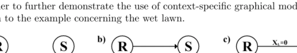
A context-specific independence is displayed in a graph by adding a label to an edge, detailing for which outcomes the context-specific independence holds. In order to further demonstrate the use of context-specific graphical models we return to the example concerning the wet lawn.
Initially, we again assume that the sprinkler system is fully automated, re-calling that the “optimal model” in this scenario is the directed graph in Figure 2a. However, now we are also equipped to consider the occurrence of context-specific independencies. Given that it is raining the lawn is highly likely to be wet independent of whether or not the sprinkler system is active, and similarly if the sprinklers are active the lawn is likely to be wet independent of whether or not it is raining. If we useXR= 1 to denote that it is raining andXS = 1 to
denote that the sprinklers are active we get the context-specific independencies
XL⊥XS|XR= 1 andXL⊥XR|XS = 1. Using the graph in Figure 4a we can
incorporate these context-specific independencies in the graphical model. Considering the scenario where the sprinkler system is only semi-automatic a third context-specific independence becomes plausible. Given that the lawn is dry (XL = 0) it is unlikely that is raining or that the sprinklers are active,
meaning that XR ⊥ XS|XL = 0. Using directed graphs these three
context-specific independences cannot be simultaneously represented and the graph in Figure 4b could be used instead. Using an undirected graph all the context-specific independencies can be displayed, as shown by the graph in Figure 4c.
Context-specific independencies can also be defined for continuous systems as shown in Nyman et al. (2014b). In this case, context-specific independencies are defined to hold not for a specific value but rather in an interval. We might, for instance, have the case that Xδ ⊥Xγ|Xω∈(0,∞).
4
Using Markov chain Monte Carlo methods to
perform model optimization
4.1
Markov chains
In this section we will review the basic theory of Markov chains required for un-derstanding Markov chain Monte Carlo methods. For a more in-depth analysis of the subject the reader is referred to, for instance, Norris (1998). A Markov chain is a sequence of stochastic variables X =X0, X1, X2, . . ., such that each variable assumes its value from the state spaceE, and
P(Xn+1=in+1|Xn=in, Xn−1=in−1, . . . , X0=i0) =
P(Xn+1=in+1|Xn=in),
for all n= 1,2, . . . andi0, i1, . . . , in+1 ∈E. We will only consider cases where the state space E is discrete, resulting in a discrete time Markov chain on a discrete state space. If it holds for allnand statesi, j∈E that
P(X1=j|X0=i) =P(Xn+1=j|Xn=i) =Pij
the Markov chain is said to be time homogeneous or stationary. Pij is called
the transition probability from stateitoj. The transition probabilities satisfy the requirement
X
j∈E
Pij = 1,
for alli∈E. The matrix P with the elementsPij, i, j∈E, is called the
tran-sition probability matrix and is said to be a stochastic matrix as each element is larger than or equal to zero and the sum of each row equals one. A time ho-mogeneous Markov chain is completely determined by its transition probability matrix and its initial distribution, which determines the probabilitiesP(X0=i), for i ∈ E. Given P the probability P(Xm =j|X0 = i) can be calculated as (Pm)
ij.
A statejis said to be accessible from stateiif there exists an integernsuch that P(Xn =j|X0 =i)> 0. A Markov chain is termed as irreducible given that any state is accessible from any other state. If from some state ino other states are accessible, i.e. P(X1 = i|X0 =i) = 1, i is said to be an absorbing state. It follows directly from the definitions that no Markov chain containing an absorbing state can be irreducible. A state i is termed aperiodic if there exists an integer m such that P(Xn = i|X0 = i) >0 for all integers n ≥m. A Markov chain is aperiodic if each state is aperiodic. A time homogeneous Markov chain is reversible if there exists a distribution λover the state space such thatλiPij=λjPji, for alli, j∈E.
A stationary distribution of a Markov chain is a row vectorπsuch thatπ=
πP. For an irreducible and aperiodic Markov chain the stationary distribution is unique. Given that the initial distribution equals the stationary distribution the following property holds
P(X0=i) =P(Xm=i) =πi, for everymandi∈E.
is due to the fact that for the described Markov chain each row ofPmtends to πasmtends to infinity, meaning thatP(Xm=i|X0=j)→πifor allj ∈Eas m→ ∞.
A wide range of interesting real life problems can be modeled using Markov chains. The example that we shall consider next is an example of the so called “Gambler’s ruin” problem. In a game you are given three dice, if you roll at least one six you win one euro, if not you lose one euro. The probability with which you lose one euro is q = (5/6)3 ≈0.58 and the probability with which you win one euro is p= 1−q ≈0.42. A man has three euros and decides to play the game until he has doubled his money or until he is broke.
In order to calculate the probability the man has of obtaining six euros we use a Markov chain to model the problem. The state space is chosen to be
E={0,1,2,3,4,5,6}, i.e. the amount of euros that the man might have at one point. As he initially has three euros the initial distribution is (0,0,0,1,0,0,0). The transition probability matrix is
P = 1 0 0 0 0 0 0 q 0 p 0 0 0 0 0 q 0 p 0 0 0 0 0 q 0 p 0 0 0 0 0 q 0 p 0 0 0 0 0 q 0 p 0 0 0 0 0 0 1 .
From P we can see that states 0 and 6 are absorbing states. This is a logi-cal result as these states translate to the man being broke or satisfied with his winnings and stops playing, respectively. The existence of the absorbing states means that the Markov chain is not irreducible. The Markov chain is not aperi-odic either as for all non-absorbing states it holds that a return to the starting state can only occur after an even number of steps. The chain is, however, reversible. This can be seen by settingλ= (a,0,0,0,0,0, b), witha+b= 1.
To solve the given problem we start by defining N = min{n : Xn =
0 orXn = 6} and ωi = P(XN = 6|X0 = i). We are interested in finding
ω3 = P(XN = 6|X0 = 3). Given the rules of the game we can deduce that
ω0 = 0, ω6 = 1, and if 1 ≤ i ≤ 5 then ωi =qωi−1+pωi+1. By solving the resulting equation system we get that
ω3=
p3−3p4q+ 2p5q2
1−6pq+ 11p2q2−6p3q3 = 0.27840. . .
Clearly, equation systems of this kind lead to rather arduous solutions even for small and simple problems like this one. Fortunately, Markov chains are often easy to model in a computer, using multiple simulations of a problem an approximation of the sought after probability, or other property, can often be found.
4.2
Markov chain Monte Carlo methods
Markov chain Monte Carlo (MCMC) methods are mainly used for two types of problems (MacKay, 2003). Firstly, to draw samples from a probability distri-bution where direct sampling is not possible but the density function can easily
be evaluated at any point. And secondly, to estimate expectations of functions under such a distribution.
One commonly used MCMC method is the Metropolis-Hastings method. By f(x) we denote the density function of the distribution from which we wish to draw a random sample. To start with, a random number x0, for which
f(x0)>0, is selected as the starting state for a Markov chain. At timet+ 1 a candidate state x∗ is generated using a proposal mechanism, Q(x∗|xt) denotes
the probability (or density) with which x∗ is selected as the candidate state given that xtis the current state. With probability
min 1, f(x ∗)Q(x t|x∗) f(xt)Q(x∗|xt) (1)
x∗is accepted as the next state and we setxt+1=x∗, otherwise we setxt+1=xt.
As an example we consider the problem where we want to draw a sample from the standardized normal distribution. The starting state is set to x0 = 0 and the proposal mechanism used is defined by x∗ =xt+y, wherey is drawn
randomly from the uniform distribution with endpoints−2 and 2. This might, for instance, result inx∗= 0.42 which would be accepted with the probability
min 1, f(x ∗)Q(x 0|x∗) f(x0)Q(x∗|x0) = f(0.42) f(0) ≈0.916.
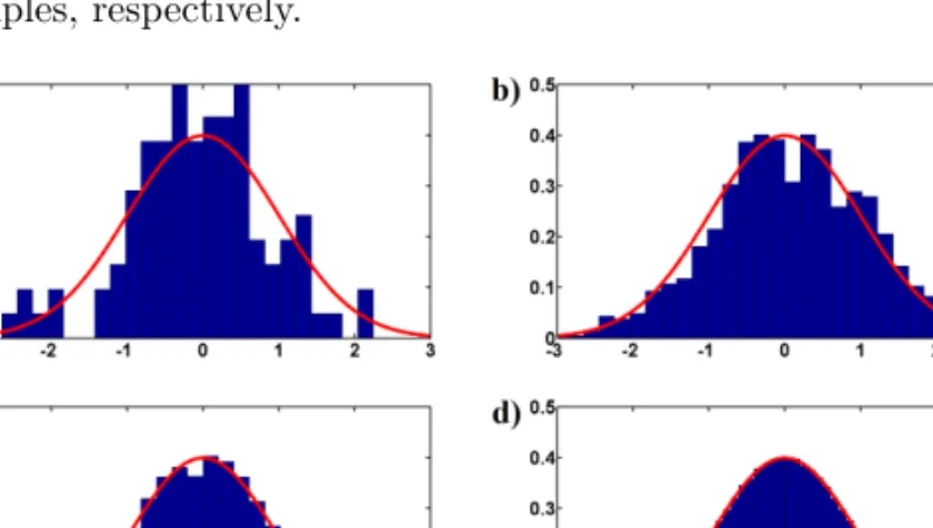
In other words, it is highly likely that the candidate state would be accepted resulting in x1 = 0.42. Continuing the Markov chain in this fashion might result in the vector (0, 0.42, 0.42, −0.15, −0.95, . . .). Although consecutive elements in this vector are not independent of each other selecting, for instance, every 20:th element will result in a sample that is effectively drawn from the standardized normal distribution. This is due to the fact that the stationary distribution of the considered reversible Markov chain equals f(x). This can be visualized by considering a histogram plotted alongside f(x) as is done in Figure 5. Figure 5a-d shows the histogram resulting from 100, 1000, 10000, and 1000000 samples, respectively.
The use of MCMC methods becomes interesting when studying graphical models and you want to find the optimal model given a dataset X. To be able to do this a score function, like the one found in for instance Nyman et al. (2014c), for a given graph is required. The score function usually contains the probability P(X|G) where Gis a graph in the considered model spaceG. The optimal graph is the graph that optimizes the posterior probability
P(G|X) = P P(X|G)P(G)
G∈GP(X|G)P(G)
,
where P(G) is a prior distribution overG. If every aspect of the posterior dis-tribution were known, it would be possible to immediately identify the optimal model, unfortunately, even the seemingly simple task of direct sampling from this distribution is intractable. Therefore, the use of an MCMC method be-comes a viable option as the density function can be evaluated asf(G) =P(G|
X)∝P(X|G)P(G).
Corander et al. (2006) and later Corander et al. (2008) showed that the process of learning the optimal graph can be made more effective by removing the factor concerning Q in the acceptance probability (1), resulting in a new acceptance probability min 1, f(x ∗) f(xt) .
Unfortunately, this leads to the Markov chain being non-reversible, and con-sequently, the stationary distribution not equaling the posterior distribution
P(G|X). However, if the focus of the problem lies in finding the model opti-mizing the posterior distribution this is not a fatal flaw. In addition, Corander et al. (2008) proved, under rather weak conditions, that the posterior probability of a graph can be consistently estimated using
ˆ Pt(G|X) = P(X|G)P(G) P G0∈G tP(X|G 0)P(G0),
whereGtis the set of graphs that has been visited by the Markov chain at time t.
5
Classification
Classifying an element based on a set of observable features (variables) as be-longing to a specific class among a set of predetermined classes, known as su-pervised classification, is one of the most common tasks considered in machine learning and statistics (Bishop, 2007; Duda et al., 2000; Hastie et al., 2009; Rip-ley, 1996). As a result, there exists a wide range of different classifiers. In this section we will consider the difference between two classifiers, the naive Bayes classifier which assumes that the features are independent given the class label and a classifier which models the dependence structure of the features using a graphical model (Nyman et al., 2014d).
An example of a classification problem, considered in Nyman et al. (2014d), is that given the answers that a candidate in the Finnish parliament elections of 2011 gave in a questionnaire, decide which party the candidate belongs to. A widely used method is the naive Bayes classifier which assumes that all the answers to the questions given by a candidate are independent of each other given that the candidate’s party is known. This leads to a simple model that is easy to work with and time-efficient. While the naive Bayes classifier has been shown to work well in practice, in some cases it can be oversimplified. For instance, a candidates opinion on gun control issues may correlate with his opinion on government spending, a correlation that the naive Bayes model does not take into account. In such a case using a graphical model to determine the dependence structure among the features for each class may increase the prediction accuracy.
Again, to illuminate the problem of classification we turn to the example with the variables rain (R) and sprinkler system (S). Given the outcomes of these two variables the problem is to determine the probability that the sprinkler system is fully automated, with the alternative being that the system is semi-automated. The notationR= 0 means that it is not raining andR= 1 that it is raining, similarly S = 0 means that the sprinklers are not active and S = 1 that they are active. For the new variable A we have that A = 0 means that the system is semi-automated andA= 1 that it is fully automated.
In a classification problem, we have two sets of data, the training data and the test data. For the test data we know which class each observation belongs to, in our case whetherA= 0 or A= 1. Using the training data, the parameters used in the selected model are tuned, for the sake of simplicity we use the maximum likelihood estimate of the parameters. For the test data the value of
Ais unknown. We generate data using the conditional distributions
P(R= 1) = 0.5, P(A= 1) = 0.5, P(S = 1|R= 1, A= 0) = 0.2, P(S = 1|R= 0, A= 0) = 0.5, P(S = 1|R= 0, A= 1) = 0.5, P(S = 1|R= 1, A= 1) = 0.5,
resulting in the joint distribution listed in Table 1.
R S A P(R, S, A) R S A P(R, S, A)
0 0 0 0.125 1 0 0 0.2
0 0 1 0.125 1 0 1 0.125
0 1 0 0.125 1 1 0 0.05
0 1 1 0.125 1 1 1 0.125
Table 1: Joint distribution used in the classification example.
accurate representationR⊥S|A= 1 andR6⊥S|A= 0. Given the training data we can approximate the distribution in Table 1, for sake of simplicity we assume that the size of the training data is extremely large and that the distribution can be perfectly recreated. Classification of the observations in the training data can be performed by calculating
P(A=a|R=r, S=s) = P(A=a, R=r, S=s)
P(R=r, S =s)
= PP(R=r, S=s|A=a)P(A=a)
a0P(R=r, S=s|A=a0)P(A=a0)
.
Using the naive Bayes method
P(R=r, S=s|A=a)
is calculated as
P(R=r|A=a)P(S=s|A=a).
Using the graphical model we consider the joint distribution ofR andS given
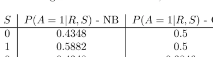
A = 0. The two methods lead to small differences in the probabilities with which an observation is assigned to the two classes, as shown in Table 2. Using
R S P(A= 1|R, S) - NB P(A= 1|R, S) - GM
0 0 0.4348 0.5
0 1 0.5882 0.5
1 0 0.4348 0.3846
1 1 0.5882 0.7142
Table 2: Probabilities with whichA= 1 givenRand S according to the naive Bayes classifier (NB) and the graphical model classifier (GM).
these probabilities when assigning an observation in the test data to a class results in the naive Bayes classifier having a success rate of 51.2% compared to 52.6% for the graphical model classifier.
6
Summaries and discussion of Articles I-V
6.1
Article I: Stratified graphical models - context-specific
independence in graphical models
The original manuscript written about stratified graphical models included much of what would later become Article I and Article III. The decision to split the material into two separate articles was made at the realization that the subject was simply too extensive to consider in a single article. Article II was conceived at roughly the same time as Article I with the difference being that Article I focuses on context-specific independence in undirected graphs and Article II on context-specific independence in directed acyclic graphs.
The ideas presented in Articles I-III are based on the work done in Corander (2003b). In that article labeled graphical models, which allow for the graphi-cal representation of context-specific independencies, are introduced. Article I introduces the concept of stratified graphical models, which also allow for the graphical representation of context-specific independencies. Different proper-ties are investigated for stratified graphical models and the term decomposable stratified graph is introduced. Decomposable stratified graphs are subject to fairly strong restriction with one of the advantages being that the induced de-pendence structure between the variables is easy to interpret. However, the main reason for introducing decomposable stratified graphs is that for these graphs the marginal likelihood of a dataset can be analytically calculated. The main contribution of this article is the introduction of a formula, based on sim-ilar works in Cooper & Herskovits (1992), Friedman & Goldszmidt (1996) and Chickering et al. (1997), for calculating the marginal likelihood of a dataset given a decomposable stratified graph.
A non-reversible MCMC approach (Corander et al., 2008, 2006) is used to identify the optimal decomposable stratified graph given a dataset. In this search a non-uniform prior is applied over the model space to penalize dense graphs as such graphs have the advantage of a wider range of parameter restric-tion compared to sparse graphs. The introduced theory is applied to a range of synthetic and real datasets with the result showing that context-specific in-dependencies occur naturally in data. Using the examples, further experiments are conducted to deduce the robustness of the inferred models. As one could expect, as the model space grows much more quickly for stratified graphs than for ordinary undirected graphs, results show that model inference is more chal-lenging for stratified graphs and larger datasets are required in order to obtain reliable results.
6.2
Article II: Labeled directed acyclic graphs: a
gener-alization of context-specific independence in directed
graphical models
This article introduces context-specific independencies to directed acyclic graphs using labeled directed acyclic graphs. Although some features are the same for stratified graphical models and labeled directed acyclic graphs, the dependence structures that can be represented vary somewhat, just as is the case for Markov networks and Bayesian networks. One such difference is that the set of
condi-differently for the two model classes.
A formula, very similar to the one used in Article I, is introduced to calcu-late the marginal likelihood of a dataset given a labeled directed acyclic graph. Model optimization is performed to identify the optimal dependence structure for a dataset. The optimization process utilizes a non-reversible MCMC method (Corander et al., 2008, 2006) combined with a greedy hill climbing method, see for instance Heckerman et al. (1995). The non-reversible MCMC method uses a Markov chain with the state space constituted by the set of all directed acyclic graphs. Given a directed acyclic graph the greedy hill climbing method is used to identify the optimal set of context-specific independencies applicable to that graph.
The problem of model identifiability is considered in the article. This prob-lem concerns labeled directed acyclic graphs that have different appearances while inducing identical parameter restrictions. Of course, model identifiability is also an issue with ordinary directed graphs as we recall that chain nodes and fork nodes are identical in terms of the marginal and conditional dependencies that they induce. One reason why model identifiability is important is that when performing model inference two graphs that might have significant dif-ferences in appearance may result in equal marginal likelihoods due to the fact that their induced dependence structures are identical.
The article also introduces a novel non-uniform prior over the model space. Just like the prior used in Article I, this prior penalizes excessive use of labels, encouraging the optimization process to express the dependence structure pri-marily using the graph and secondarily using labels. To deduce the effect of the prior distribution experiments are performed under priors of varying strength for a range of sample sizes.
6.3
Article III: Context-specific independence in
graphi-cal log-linear models
As previously mentioned this article and Article I were at first intended to be part of the same manuscript as they cover roughly the same subject, stratified graphical models. The article starts by covering the basic properties of stratified graphical models that were introduced in Article I. However, as the name of the article suggests, the emphasis is then moved to graphical log-linear models (Lau-ritzen, 1996; Whittaker, 1990) and the restrictions imposed by context-specific independencies to the log-linear parameterization. A number of theorems con-cerning the properties of stratified graphs and the log-linear parameterization is presented. Perhaps the most interesting of these theorems shows that some stratified graphs induce non-hierarchical models, a class of models that Whit-taker (1990) deemed as “. . . not necessarily uninteresting; it is just that the focus of interest is something other than independence”.
In Article I, we introduced decomposable stratified graphs to enable the calculation of the marginal likelihood of a dataset. Here we use an alternative method for model scoring, the Bayesian information criterion (Schwarz, 1978). This score function requires that the maximum likelihood estimate of the model parameters can be calculated given any model in the model space. A method is used where the maximum likelihood estimate, attained without imposing any restrictions, is cyclically projected to fulfill one parameter restriction at a time until the process converges. Using this method it is shown that the desired
probability distribution can be attained while removing most of the restrictions imposed by decomposable stratified graphs. The method of cyclical projection is based on the general works of Csisz´ar (1975) and Csisz´ar & Mat´u˘s (2003), and Corander (2003a) and Rudas (1998) who used the same method for non-chordal undirected graphs.
Model optimization, using the Bayesian information criterion to approxi-mate the marginal likelihood, is performed on some of the same datasets as in Article I. While the results are similar it is clear that removing the restrictions introduced for decomposable stratified graphs further increases the model space and differences between the inferred models do exist.
6.4
Article IV: Stratified Gaussian graphical models
The aim of this article is to translate stratified graphical models to the continu-ous setting, creating a new model class termed as stratified Gaussian graphical models. The obvious approach is to apply context-specific independencies to Gaussian graphical models, which constitute the preferred class of models when analyzing continuous multivariate systems, see for instance Dempster (1972), Giudici & Green (1999), and Atay-Kayis & Massam (2005). This is a novel ap-proach as context-specific independencies have previously not been considered for Gaussian graphical models.
The article begins by reviewing the basic concepts of Gaussian graphical models and discrete stratified graphical models. Next, context-specific indepen-dencies are introduced for continuous variables. While most of the properties found for stratified graphical models are also valid in the continuous setting, due to the restrictive nature of the multivariate Gaussian distribution some features are a bit more complicated to deal with. One such feature concerns interpret-ing the dependence structure in the presence of multiple context-specific inde-pendencies. The introduced algorithm used for this purpose involves imposing the restrictions of a decomposable stratified graph, transforming all included context-specific independencies to the discrete setting, where the dependence structure can be readily determined, and then transforming back to the con-tinuous setting. The result is a partitioning of the joint outcome space of the included variables, such that each part is associated with its own dependence structure in the form of an undirected graph.
Given that the dependence structure induced by the inclusion of context-specific independencies can be readily determined, a family of probability den-sity functions, using the same parameters as a multivariate Gaussian distribu-tion, can be found for each continuous stratified graph. It is proved in the article that the density functions belong to the curved exponential family. This is of relevance as Haughton (1988) showed that for density functions belonging to the curved exponential family model selection using the Bayesian information criterion (Schwarz, 1978) produces consistent results.
One of the datasets considered in the article contains the marks received by students in different areas of mathematics. The dataset has been analyzed by numerous different sources (Edwards, 2000; Mardia et al., 1979; Whittaker, 1990) with the general consensus regarding the marginal and conditional de-pendencies matching the ones identified in this article. However, using the introduced theory of stratified Gaussian graphical models, evidence supporting
discovered.
6.5
Article V: Marginal and simultaneous classification
using stratified graphical models
The concept of this article is to use the theory from Article I to construct a predictive classifier. The considered classifier is a supervised classifier as it is assumed that the total number of classes is known before any data is regarded. As the posterior distribution of the class labels is attained via first modeling the joint distribution of the class labels and variables conditional on the training data, rather than directly modeling the posterior distribution of the class labels, the classifier is termed a generative classifier.
When creating the classifier we operate under the assumption that the de-pendence structure among the variables varies from class to class, contrary to the dependence structure being identical for each class or the variables being independent given the class label. In some cases, it is possible that the different dependence structures are known beforehand, but a more realistic scenario is that the dependence structure needs to be learned using the available training data. The question, whether or not it is better to consider the variables depen-dent of each other or not, has received substantial attention over the years. For instance, Friedman et al. (1997) concluded that modeling the dependence struc-ture using Bayesian networks did not improve the performance of the classifier compared to naive Bayes classifiers which considers the variables as indepen-dent of each other. However, Madden (2009) later concluded that the results by Friedman et al. (1997) where due to use of maximum likelihood estimation of the parameters and that smoothing the estimated parameters with a prior could in some cases result in a greatly improved classification accuracy.
Two separate types of classifiers are considered, a marginal classifier and a simultaneous classifier (Corander et al., 2013). For the marginal classifier, all observations in the test data are treated separately, i.e. assigned to a class independently of the other observations in the test data. For the simultaneous classifier, all observations in the test data are considered simultaneously, mean-ing that assignmean-ing one observation to a certain class will affect the probability of assigning any other observation to that class.
Simultaneous and marginal classifiers are implemented using both ordinary undirected graphs and decomposable stratified graphs to encode the dependence structure. Experiments using synthetic data show the vast potential that the considered classifiers have of improving classification accuracy compared to, for instance, the naive Bayes classifier. Experiments on real datasets confirm that the introduced classifiers clearly outperform the out-of-the-box classifiers to which they are compared.
References
Atay-Kayis, A. & Massam, H. (2005). A Monte Carlo method for comput-ing the marginal likelihood in nondecomposable Gaussian graphical models. Biometrika92, 317–335.
Bishop, C. M. (2007). Pattern Recognition and Machine Learning. New York: Springer.
Boutilier, C., Friedman, N., Goldszmidt, M. & Koller, D. (1996). Context-specific independence in Bayesian networks. In Proceedings of the Twelfth Annual Conference on Uncertainty in Artificial Intelligence, 115–123. Chickering, D. M., Heckerman, D. & Meek, C. (1997). A Bayesian approach
to learning Bayesian networks with local structure. In Proceedings of the Thirteenth Annual Conference on Uncertainty in Artificial Intelligence, 80– 89.
Cooper, G. F. & Herskovits, E. (1992). A Bayesian method for the induction of probabilistic networks from data. Machine learning9, 309–347.
Corander, J. (2003a). Bayesian graphical model determination using decision theory. Journal of multivariate analysis85, 253–266.
Corander, J. (2003b). Labelled graphical models. Scandinavian Journal of Statistics30, 493–508.
Corander, J., Cui, Y., Koski, T. & Sir´en, J. (2013). Have I seen you before? Principles of Bayesian predictive classification revisited. Statistics and Com-puting 23, 59–73.
Corander, J., Ekdahl, M. & Koski, T. (2008). Parallell interacting MCMC for learning of topologies of graphical models. Data Mining and Knowledge Discovery17, 431–456.
Corander, J., Gyllenberg, M. & Koski, T. (2006). Bayesian model learning based on a parallel MCMC strategy. Statistics and Computing16, 355–362. Csisz´ar, I. (1975). I-divergence geometry of probability distributions and
mini-mization problems. The Annals of Probability3, 146–158.
Csisz´ar, I. & Mat´u˘s, F. (2003). Information projections revisited. IEEE Trans-actions on Information Theory49, 1474–1490.
Darroch, J. N., Lauritzen, S. L. & Speed, T. (1980). Markov fields and log-linear interaction models for contingency tables. The Annals of Statistics 522–539. Dempster, A. (1972). Covariance selection. Biometrics 28, 157–175.
Duda, R. O., Hart, P. E. & Stork, D. G. (2000). Pattern Classification, 2nd edn. New York: Wiley.
Edwards, D. (2000). Introduction to Graphical Modelling (2nd ed.). New York: Springer-Verlag.
Eriksen, P. S. Context specific interaction models. Technical report, Department of Mathematical Sciences, Aalborg University, Aalborg (1999).
Eriksen, P. S. Decomposable log-linear models. Technical report, Department of Mathematical Sciences, Aalborg University, Aalborg (2005).
Friedman, N., Geiger, D. & Goldszmidt, M. (1997). Bayesian network classifiers. Machine Learning 29, 131–163.
Friedman, N. & Goldszmidt, M. (1996). Learning Bayesian networks with local structure. In Proceedings of the Twelfth Annual Conference on Uncertainty in Artificial Intelligence, 252–262.
Giudici, P. & Green, P. (1999). Decomposable graphical Gaussian model deter-mination. Biometrika86, 785–801.
Hastie, T., Tibshirani, R. & Friedman, J. (2009). The Elements of Statisti-cal Learning: Data Mining, Inference, and Prediction, 2nd edn. New York: Springer.
Haughton, D. (1988). On the choice of a model to fit data from an exponential family. The Annals of Statistics16, 342–355.
Heckerman, D., Geiger, D. & Chickering, D. M. (1995). Learning Bayesian net-works: The combination of knowledge and statistical data. Machine Learning
20, 197–243.
Højsgaard, S. (2003). Split models for contingency tables. Computational Statis-tics & Data Analysis42, 621–645.
Højsgaard, S. (2004). Statistical inference in context specific interaction models for contingency tables. Scandinavian Journal of Statistics31, 143–158. Koller, D. & Friedman, N. (2009).Probabilistic graphical models: principles and
techniques. London: The MIT Press.
Koski, T. & Noble, J. (2009).Bayesian networks: an introduction. Chippenham: Wiley.
Lauritzen, S. L. (1996). Graphical models. Oxford: Oxford University Press. Lauritzen, S. L. & Wermuth, N. (1989). Graphical models for associations
between variables, some of which are qualitative and some quantitative. The Annals of Statistics 31–57.
MacKay, D. J. C. (2003). Information theory, inference, and learning algo-rithms. Cambridge: Cambridge University Press.
Madden, M. G. (2009). On the classification performance of TAN and general Bayesian networks. Knowledge-Based Systems22, 489–495.
Mardia, K. V., Kent, J. T. & Bibby, J. M. (1979). Multivariate Analysis. Lon-don: Academic Press.
Nyman, H., Pensar, J. & Corander, J. (2014a). Context-specific independence in graphical log-linear models. arXiv:1409.2713 [stat.ML] .
Nyman, H., Pensar, J. & Corander, J. (2014b). Stratified Gaussian graphical models. arXiv:1409.2262 [math.ST] .
Nyman, H., Pensar, J., Koski, T. & Corander, J. (2014c). Stratified graphical models - context-specific independence in graphical models. Bayesian Analysis doi:10.1214/14-BA882.
Nyman, H., Xiong, J., Pensar, J. & Corander, J. (2014d). Marginal and simultaneous predictive classification using stratified graphical models. arXiv:1401.8078 [stat.ML] .
Pensar, J., Nyman, H., Koski, T. & Corander, J. (2014). Labeled directed acyclic graphs: a generalization of context-specific independence in directed graphical models. Data Mining and Knowledge Discovery doi:10.1007/s10618-014-0355-0.
Ripley, B. D. (1996). Pattern Recognition and Neural Networks. Cambridge: Cambridge University Press.
Rudas, T. (1998). A new algorithm for the maximum likelihood estimation of graphical log-linear models. Computational Statistics 13, 529–537.
Schwarz, G. (1978). Estimating the dimension of a model. The Annals of Statistics6, 461–464.
Whittaker, J. (1990).Graphical models in applied multivariate statistics. Chich-ester: Wiley.