DOI 10.1007/s11634-008-0020-9
R E G U L A R A RT I C L E
SVM-Maj: a majorization approach to linear support
vector machines with different hinge errors
P. J. F. Groenen · G. Nalbantov · J. C. Bioch
Received: 3 November 2007 / Revised: 23 February 2008 / Accepted: 25 February 2008 Published online: 27 March 2008
© The Author(s) 2008
Abstract Support vector machines (SVM) are becoming increasingly popular for
the prediction of a binary dependent variable. SVMs perform very well with respect to competing techniques. Often, the solution of an SVM is obtained by switching to the dual. In this paper, we stick to the primal support vector machine problem, study its effective aspects, and propose varieties of convex loss functions such as the standard for SVM with the absolute hinge error as well as the quadratic hinge and the Huber hinge errors. We present an iterative majorization algorithm that minimizes each of the adaptations. In addition, we show that many of the features of an SVM are also obtained by an optimal scaling approach to regression. We illustrate this with an example from the literature and do a comparison of different methods on several empirical data sets.
Keywords Support vector machines·Iterative majorization·Absolute hinge error·
Quadratic hinge error·Huber hinge error·Optimal scaling
Mathematics Subject Classification (2000) 90C30·62H30·68T05
P. J. F. Groenen (
B
)·J. C. BiochEconometric Institute, Erasmus University Rotterdam, P. O. Box 1738, 3000 DR, Rotterdam, The Netherlands e-mail: [email protected]
J. C. Bioch
e-mail: [email protected] G. Nalbantov
ERIM and Econometric Institute, Erasmus University Rotterdam, P. O. Box 1738, 3000 DR, Rotterdam, The Netherlands e-mail: [email protected]
1 Introduction
An increasingly more popular technique for the prediction of two groups from a set of predictor variables is the support vector machines (SVM, see, e.g.,Vapnik 2000). Although alternative techniques such as linear and quadratic discriminant analysis, neural networks, and logistic regression can also be used to analyze this data analysis problem, the prediction quality of SVMs seems to compare favorably with respect to these competing models. Another advantage of SVMs is that they are formulated as a well-defined optimization problem that can be solved through a quadratic program. A second valuable property of the SVM is that the derived classification rule is relatively simple and can be readily applied to new, unseen samples. A potential disadvantage is that the interpretation in terms of the predictor variables in nonlinear SVM is not always possible. In addition, the usual dual formulation of an SVM may not be so easy to grasp.
In this paper, we restrict our focus to linear SVMs. We believe that this paper makes several contributions on three themes. First, we offer a nonstandard way of looking at linear SVMs that makes the interpretation easier. To do so, we stick to the primal problem and formulate the SVM in terms of a loss function that is reg-ularized by a penalty term. From this formulation, it can be seen that SVMs use robustified errors. Apart from the standard SVM loss function that uses the absolute hinge error, we advocate two other hinge errors, the Huber and quadratic hinge errors, and show the relation with ridge regression. Note that recently, Rosset and Zhu (2007) also discusses the use of different errors in SVMs including these two hinge errors.
The second theme of this paper is to show the connection between optimal scaling regression and SVMs. The idea of optimally transforming a variable so that a criterion is being optimized has been around for more than 30 years (see, e.g.,Young 1981; Gifi 1990). We show that optimal scaling regression using an ordinal transformation with the primary approach to ties comes close to the objective of SVMs. We discuss the similarities between both approaches and give a formulation of SVM in terms of optimal scaling.
A third theme is to develop and extend the majorization algorithm ofGroenen et al. (2007) to minimize the loss for any of the hinge errors. We call this general algorithm SVM-Maj. The advantage of majorization is that each iteration is guaranteed to reduce the SVM loss function until convergence is reached. As the SVM loss functions with convex hinge errors such as the quadratic and Huber hinge errors are convex, the majorization algorithm stops at a minimum after a sufficient number of iterations. For the case of the Huber and quadratic hinge, the SVM-Maj algorithm turns out to yield computationally very efficient updates amounting to a single matrix multiplication per iteration. Through SVM-Maj, we contribute to the discussion on how to approach the linear SVM quadratic problem.
Finally, we provide numerical experiments on a suite of 14 empirical data sets to study the predictive performance of the different errors in SVMs and compare it to optimal scaling regression. We also compare the computational efficiency of the majorization approach for the SVM to several standard SVM solvers.
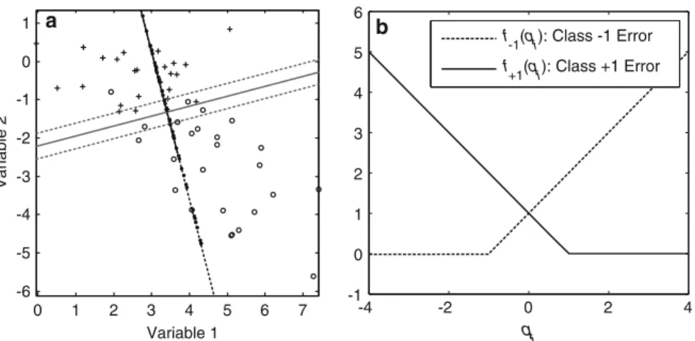
0 1 2 3 4 5 6 7 -6 -5 -4 -3 -2 -1 0 1 Variable 1 Variable 2 -4 -2 0 2 4 -1 0 1 2 3 4 5 6 q i f -1(qi): Class -1 Error f+1(qi): Class +1 Error b a
Fig. 1 a Projections of the observations in groups 1 (+) and−1 (o) onto the line given byw1andw2.
b The absolute hinge error function f1(qi)for class 1 objects (solid line) and f−1(qi)for class−1 objects
(dashed line)
2 The SVM loss function
Here, we present a rather non-mainstream view on explaining how SVM work. There is a quite close relationship between SVM and regression. We first introduce some notation. Let the matrix of quantitative predictor variables be represented by the n×m
matrix X of n objects and m variables. The grouping of the objects into two classes is given by the n×1 vector y, that is, yi = 1 if object i belongs to class 1 and
yi = −1 if object i belongs to class−1. The exact labeling−1 and 1 to distinguish
the classes is not important. The weights used to make a linear combination of the predictor variables is represented by the m×1 vector w. Then, the predicted value qi
for object i is
qi =c+xiw, (1)
where xi is row i of X and c is an intercept. As an illustrative example, consider Fig.1a with a scatterplot of two predictor variables, where each row i is represented by a point labelled ‘+’ for the class 1 and ‘o’ for class−1. Every combination ofw1and
w2defines a direction in this scatter plot. Then, each point i can be projected onto this line. The main idea of the SVM is to choose this line in such a way that the projections of the points of class 1 are well separated from those of class−1. The line of separation is orthogonal to the line with projections and the intercept c determines where exactly it occurs. The lengthwof w has the following significance. If w has length 1, that is,w = (ww)1/2 = 1, then Fig.1a explains fully the linear combination (1). If
w does not have length 1, then the scale values along the projection line should be
multiplied byw. The dotted lines in Fig.1a show all those points that project to the lines at qi = −1 and qi =1. These dotted lines are called the margin lines in SVMs.
With three predictor variables, the objects are points in a three dimensional space,
form a plane and in higher dimensionality form a hyperplane. Thus, with more than two predictor variables, there will be a separation hyperplane and the margins are also hyperplanes. Summarizing, the SVM has three sets of parameters that determine its solution: (1) the weights normalized to have length 1, that is, w/w, (2) the length of w, that is,w, and (3) the intercept c.
An error is counted in SVMs as follows. Every object i from class 1 that projects such that qi ≥1 yields a zero error. However, if qi <1, then the error is linear with
1−qi. Similarly, objects in class−1 with qi ≤ −1 do not contribute to the error,
but those with qi >−1 contribute linearly with qi+1. Thus, objects that project on
the wrong side of their margin contribute to the error, whereas objects that project on the correct side of their margin yield zero error. Figure1b shows the error functions for the two classes. Because of its hinge form, we call this error function the absolute
hinge error.
As the length of w controls how close the margin lines are to each other, it can be beneficial for the number of errors to choose the largestwpossible, so that fewer points contribute to the error. To control thew, a penalty term that is dependent onwis added to the loss function. The penalty term also avoids overfitting of the data.
Let G1and G−1respectively denote the sets of class 1 and−1 objects. Then, the SVM loss function can be written as
LSVM(c,w) =i∈G1max(0,1−qi)+ i∈G−1max(0,qi +1)+λw w =i∈G1 f1(qi) + i∈G−1 f−1(qi) +λw w
=Class 1 errors +Class−1 errors +Penalty for
nonzero w,
(2)
whereλ >0 determines the strength of the penalty term. In this notation, the arguments
(c,w)indicate that LSVM(c,w)needs to be minimized with respect to the arguments
c and w. For similar expressions, seeHastie et al.(2001) andVapnik(2000). Note that (2) can also be expressed as
LSVM(c,w)=
n
i=1
max(0,1−yiqi)+λww,
which is closer to the expressions used in the SVM literature.
Once a solution c and w is found that minimizes (2), we can determine how each object contributes to the error. Each object i that projects on the correct side of its mar-gin contributes with zero error to the loss. Therefore, these objects could be removed from the analysis without changing the minimum of (2) and the values of c and w where this minimum is reached. The only objects determining the solution are those projecting on or at the wrong side of their margin thereby inducing error. Such objects are called support vectors as they form the fundament of the SVM solution. Unfor-tunately, these objects (the support vectors) are not known in advance and, therefore, the analysis needs to be carried out with all n objects present in the analysis. It is the
very essence of the SVM definition that error free data points have no influence on the solution.
From (2) it can be seen that any error is punished linearly, not quadratically. There-fore, SVMs are more robust against outliers than a least-squares loss function. The idea of introducing robustness by absolute errors is not new. For more information on robust multivariate analysis, we refer toHuber(1981),Vapnik(2000), andRousseeuw and Leroy(2003). In the next section, we discuss two other error functions, one of which is robust.
In the SVM literature, the SVM loss function is usually presented as follows (Burges 1998): LSVMClas(c,w, ξ)=C i∈G1 ξi+C i∈G2 ξi + 1 2w w, (3) subject to 1+(c+wxi)≤ξi for i ∈G−1 (4) 1−(c+wxi)≤ξi for i ∈G1 (5) ξi ≥0, (6)
where C is a nonnegative parameter set by the user to weigh the importance of the errors represented by the so-called slack variablesξi. If object i in G1projects at the
correct side of its margin, that is, qi =c+wxi ≥1, then 1−(c+wxi)≤0 so that
the correspondingξi can be chosen as 0. If i projects on the wrong side of its margin,
then qi =c+wxi <1 so that 1−(c+wxi) >0. Choosingξi =1−(c+wxi)gives the
smallestξisatisfying the restrictions in (4), (5), and (6). Therefore,ξi =max(0,1−qi)
and is a measure of error. For class−1 objects, a similar derivation can be made. Note that in the SVM literature (3) and (6) are often expressed more compactly as
LSVMClas(c,w, ξ)=C n i=1 ξi+ 1 2w w, subject to yi(c+wxi)≤1−ξi for i =1, . . . ,n ξi ≥0. If we choose C as(2λ)−1then LSVMClas(c,w, ξ) =(2λ)−1 ⎛ ⎝ i∈G1 ξi+ i∈G−1 ξi+2λ 1 2w w ⎞ ⎠ =(2λ)−1 ⎛ ⎝ i∈G1 max(0,1−qi)+ i∈G−1 max(0,qi+1)+λww ⎞ ⎠ =(2λ)−1L (c,w).
-4 -2 0 2 4 -1 0 1 2 3 4 5 6 -4 -2 0 2 4 -1 0 1 2 3 4 5 6 -4 -2 0 2 4 -1 0 1 2 3 4 5 6 -4 -2 0 2 4 -1 0 1 2 3 4 5 6 a
Absolute hinge error
c
b
d
Quadratic hinge error
Quadratic error Huber hinge error
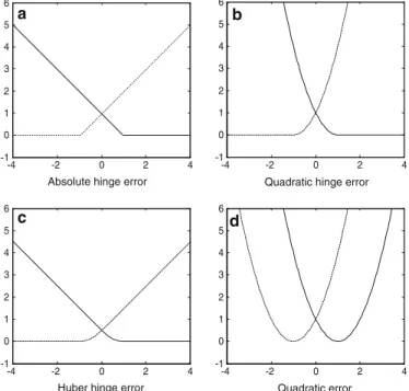
Fig. 2 Four error functions: a the absolute hinge error, b the quadratic hinge error, c the Huber hinge error,
and d the quadratic error
showing that the two formulations (2) and (3) are exactly the same up to a scaling factor(2λ)−1and yield the same c and w. The advantage of (2) lies in that it can be interpreted as a (robust) error function with a penalty. This quadratic penalty term is used for regularization much in the same way as in ridge regression, that is, to force thewj to be close to zero. The penalty is particularly useful to avoid overfitting.
Furthermore, it can be easily seen that LSVM(c,w)is a convex function in c and w as all three terms are convex in c and w. The minimum of LSVM(c,w)must be a global one as the function is convex and bounded below by zero. Note that the formulation in (3) allows the problem to be treated as a quadratic program. However, in Sect.5, we optimize (2) directly by the method of iterative majorization.
3 Other error functions
An advantage of clearly separating error from penalty is that it is easy to apply other error functions. Instead of the absolute hinge error in Fig.2a, we can use different definitions for the errors f1(qi) and f−1(qi). A straightforward alternative for the
absolute hinge error is the quadratic hinge error, see Fig.2b. This error simply squares the absolute hinge error, yielding the loss function
LQ−SVM(c,w)= i∈G1 max(0,1−qi)2+ i∈G−1 max(0,qi +1)2+λww, (7)
Table 1 Definition of error functions that can be used in the context of SVMs
Error f−1(qi)
Absolute hinge max(0,qi+1) Quadratic hinge max(0,qi+1)2
Huber hinge h−1(qi)=(1/2)(k+1)−1max(0,qi+1)2 if qi≤k
h−1(qi)=qi+1−(k+1)/2 if qi>k
Quadratic (qi+1)2
f+1(qi)
Absolute hinge max(0,1−qi) Quadratic hinge max(0,1−qi)2
Huber hinge h+1(qi)=1−qi−(k+1)/2 if qi≤ −k
h+1(qi)=(1/2)(k+1)−1max(0,1−qi)2 if qi>−k
Quadratic (1−qi)2
see also,Vapnik(2000) andCristianini and Shawe-Taylor(2000). It uses the quadratic error for objects that have prediction error and zero error for correctly predicted objects. An advantage of this loss function is that both error and penalty terms are quadratic. In Sect.5, we see that the majorizing algorithm is very efficient because in each iteration a linear system is solved very efficiently. A disadvantage of the quadratic hinge error is that outliers can have a large influence on the solution.
An alternative that is smooth and robust is the Huber hinge error, see Fig.2c. This hinge error was called “Huberized squared hinge loss” byRosset and Zhu (2007). Note thatChu et al.(2003) proposed a similar function for support vector regression. The definition of the Huber hinge is found in Table1and the corresponding SVM problem is defined by LH−SVM(c,w)= i∈G1 h+1(qi)+ i∈G−1 h−1(qi)+λww. (8)
The Huber hinge error is characterized by a linearly increasing error if the error is large, a smooth quadratic error for errors between 0 and the linear part, and zero for objects that are correctly predicted. The smoothness is governed by a value k≥ −1. The Huber hinge approaches the absolute hinge for k ↓ −1, so that the Huber hinge SVM loss solution can approach the classical SVM solution. If k is chosen too large, then the Huber hinge error essentially approaches the quadratic hinge function. Thus, the Huber hinge error can be seen as a compromise between the absolute and quadratic hinge errors. As we will see in Sect.5, it is advantageous to choose k sufficiently large, for example, k =1, as is done in Fig.2c. A similar computational efficiency as for the quadratic hinge error is also available for the Huber hinge error.
In principle, any robust error can be used. To inherit as much of the nice properties of the standard SVM it is advantageous that the error function has two properties: (1) if the error function is convex in q (and hence in w), then the total loss function
is also convex and hence has a global minimum that can be reached, (2) the error function should be asymmetric and have the form of a hinge so that objects that are predicted correctly induce zero error.
In Fig.2d the quadratic error is used, defined in Table1. The quadratic error alone simply equals a multiple regression problem with a dependent variable yi = −1 if
i ∈G−1and yi =1 if i ∈G1, that is,
LMReg(c,w)= i∈G1 (1−qi)2+ i∈G−1 (1+qi)2+λww = i∈G1 (yi−qi)2+ i∈G−1 (yi −qi)2+λww = i (yi −c−xiw) 2+λ ww = y−c1−Xw2+λww. (9) Note that for i ∈G−1we have the equality(1+qi)2=((−1)(1+qi))2=(−1−qi)2= (yi −qi)2. LMReg(c,w)has been extensively discussed inSuykens et al.(2002). To show that (9) is equivalent to ridge regression, we center the columns of X and use
JX with J=I−n−111being the centering matrix. Then (9) is equivalent to
LMReg(c,w)= y−c1−JXw2n−111+ y−c1−JXw2J+λww
= y−c12n−111+ Jy−JXw
2+λ
ww, (10) where the norm notation is defined as Z2
A = tr ZAZ = n i=1 n j=1 K k=1ai j
zi kzj k. Note that (10) is a decomposition in three terms with the intercept c appearing
alone in the first term so that it can be estimated independently of w. The optimal c in (10) equals n−11y. The remaining optimization of (10) in w simplifies into a standard ridge regression problem. Hence, the SVM with quadratic errors is equivalent to ridge regression. As the quadratic error has no hinge, even properly predicted objects with
qi < −1 for i ∈ G−1or qi > 1 for i ∈ G1 can receive high error. In addition, the quadratic error is nonrobust, hence can be sensitive to outliers. Therefore, ridge regression is more restrictive than the quadratic hinge error and expected to give worse predictions in general.
4 Optimal scaling and SVM
Several ideas that are used in SVMs are not entirely new. In this section, we show that the application of optimal scaling known since the 1970s has almost the same aim as the SVM. Optimal scaling in a regression context goes back to the models MONANOVA (Kruskal 1965), ADDALS (Young et al. 1976a), MORALS (Young et al. 1976b), and, more recently, CatREG (Van der Kooij et al. 2006;Van der Kooij 2007). The main idea of optimal scaling regression (OS-Reg) is that a variable y is replaced by an optimally transformed variabley. The regression loss function is not
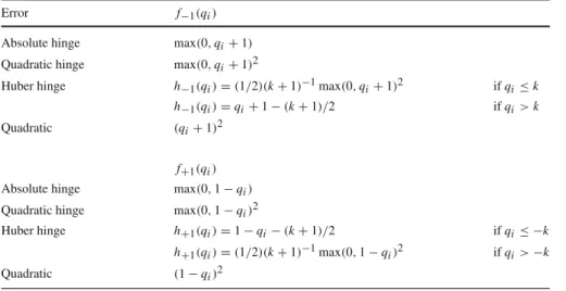
-2 -1 0 1 2 -3 -2 -1 0 1 2 3 qi y i -2 -1 0 1 2 -3 -2 -1 0 1 2 3 qi y ^ i a approach to ties b ^
Optimal scaling transformation for SVMs Optimal scaling transformation by primary
Fig. 3 Optimal scaling transformationy of the dependent variable y. a An example transformation for the
OS-Reg, b An example transformation for SVM
only optimized over the usual weights, but also over the optimally scaled variabley.
Many transformations are possible, see, for example,Gifi(1990). However, to make OS-Reg suitable for the binary classification problem, we use the so-called ordinal transformation with the primary approach to ties that allows to untie the tied data. This transformation was proposed in the context of multidimensional scaling to optimally scale the ordinal dissimilarities. As we are dealing with two groups only, this means that the only requirement is to constrain allyi in G−1to be smaller than or equal to allyj in G1. An example of such a transformation is given in Fig.3a.
OS-Reg can be formalized by minimizing
LOS−Reg(y,w)=
n
i=1
(yi −xiw)2+λww= y−Xw2+λww (11)
subject toyi ≤yj for all combinations of i ∈ G−1and j ∈ G1andyy = n. The latter requirement is necessary to avoid the degenerate zero-loss solution ofy=0 and w=0. Without loss of generality, we assume that X is column centered here. In the
usual formulation, no penalty term is present in (11), but here we add it because of ease of comparison with SVMs.
The error part of an SVM can also be expressed in terms of an optimally scaled variabley. Then, the SVM loss becomes
LSVM−Abs(y,w,c)=
n
i=1
|yi −xiw−c| +λww (12)
subject toyi ≤ −1 if i∈G−1andyi ≥1 if i∈G1. Clearly, for i∈G−1a zero error is obtained if xiw+c≤ −1 by choosingyi =xiw+c. If xiw+c>−1, then the
restrictionyi ≤ −1 becomes active so thatyimust be chosen as−1. Similar reasoning
holds for i∈G1, whereyi =xiw+c if xiw+c≥1 (yielding zero error) andyi =1
Just as the SVM, OS-Reg also has a limited number of support vectors. All objects
i that are below or above the horizontal line yield zero error. All objects i that are
have a valueyi that is on the horizontal line generally give error, hence are support
vectors.
The resemblances of SVM and OS-Reg is that both can be used for the binary classification problem, both solutions only use the support vectors, and both can be expressed in terms of an optimal scaled variabley. Although, the SVM estimates
the intercept c, OS-Reg implicitly estimates c by leaving the position free where the horizontal line occurs, whereas the SVM attains this freedom by estimating c. One of the main differences is that OS-Reg uses squared error whereas SVM uses the absolute error. Also, in its standard formλ=0 so that OS-Reg does not have a penalty term. A final difference is that OS-Reg solves the degenerate zero loss solution ofy=0 and w=0 by imposing the length constraintyy=n whereas the SVM does this through
setting a minimum difference of 2 betweenyi andyj if i and j are from different
groups.
In some cases withλ=0, we found occasionally OS-Reg solutions where one of the groups collapsed at the horizontal line and the some objects of the other group were split into two points: one also at the horizontal line, the other at a distinctly different location. In this way, the length constraint is satisfied, but it is hardly possible to distinguish the groups. Fortunately, these solutions do not occur often and they never occurred with an active penalty term (λ >0).
5 SVM-Maj: a majorizing algorithm for SVM with robust hinge errors
The SVM literature often solves the SVM problem by changing to the dual of (3) and expressing it as a quadratic program that subsequently is solved by special quadratic program solvers. A disadvantage of these solvers is that they may become computa-tionally slow for large number of objects n (although fast specialized solvers exist). Here, we use a different minimization approach based on iterative majorization (IM) algorithm applied to the primal SVM problem. One of the advantages of IM algo-rithms is that they guarantee descent, that is, in each iteration the SVM loss function is reduced until no improvement is possible. As the resulting SVM loss function for each of the three hinge errors is convex, the IM algorithm will stop when the estimates are sufficiently close to the global minimum. The combination of these properties forms the main strength of the majorization algorithm. In principle, a majorization algorithm can be derived for any error function that has a bounded second derivative as most robust errors have.
The general method of iterative majorization can be understood as follows. Let
f(q)be the function to be minimized. Then, iterative majorization makes use of an auxiliary function, called the majorizing function g(q,q), that is dependent on q and the previous (known) estimate q. There are requirements on the majorizing function
g(q,q): (1) it should touch f at the supporting point y, that is, f(q) = g(q,q), (2) it should never be below f , that is, f(q) ≤ g(q,q), and (3) g(q,q)should be simple, preferably linear or quadratic in q. Let q∗be such that g(q∗,q)≤g(q,q), for example, by choosing q∗ =arg minqg(q,q∗). As the majorizing function is never
below the original function, we obtain the so called sandwich inequality
f(q∗)≤g(q∗,q)≤g(q,q)= f(q).
This chain of inequalities shows that the update q∗obtained by minimizing the majoriz-ing function never increases f and usually decreases it. This constitutes a smajoriz-ingle iteration. By repeating these iterations, a monotonically nonincreasing (generally a decreasing) series of loss function values f is obtained. For convex f and after a suffi-cient number of iterations, the IM algorithm stops at a global minimum. More detailed information on iterative majorization can be found inDe Leeuw(1994),Heiser(1995), Lange et al.(2000),Kiers(2002), andHunter and Lange(2004) and an introduction inBorg and Groenen(2005).
An additional property of IM is useful for developing the algorithm. Suppose we have two functions, f1(q)and f2(q), and each of these functions can be majorized, that is, f1(q)≤g1(q,q)and f2(q)≤g1(q,q). Then, the function f(q)= f1(q)+f2(q) can be majorized by g(q) = g1(q,q)+g2(q,q)so that the following majorizing inequality holds:
f(q)= f1(q)+ f2(q)≤g1(q,q)+g2(q,q)=g(q,q).
For notational convenience, we refer in the sequel to the majorizing function as g(q)
without the implicit argument q.
To find an algorithm, we need to find a majorizing function for (2). For the moment, we assume that a quadratic majorizing function exists for each individual error term of the form
f−1(qi)≤a−1iqi2−2b−1iqi+c−1i =g−1(qi) (13)
f1(qi)≤a1iqi2−2b1iqi+ci =g1(qi). (14)
Then, we combine the results for all terms and come up with the total majorizing function that is quadratic in c and w so that an update can be readily derived. In the next subsection, we derive the SVM-Maj algorithm for general hinge errors assuming that (13) and (14) are known for the specific hinge error. In the appendix, we derive
g−1(qi)and g1(qi)for the absolute, quadratic, and Huber hinge error SVM.
5.1 The SVM-Maj algorithm
Equation (2) was derived with the absolute hinge error in mind. Here, we generalize the definitions of the error functions f−1(q)and f1(q)in (2) to be any of the three hinge errors discussed above so that LQ−SVMand LH−SVMbecome special cases of
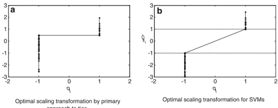
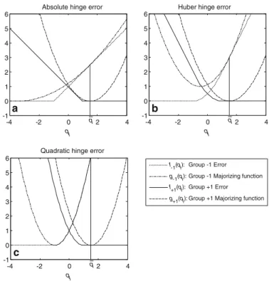
LSVM. For deriving the SVM-Maj algorithm, we assume that (13) and (14) are known for these hinge losses. Figure4shows that this is the case indeed. Then, let
f-1(qi): Group -1 Error
g-1(qi): Group -1 Majorizing function
f+1(qi): Group +1 Error
g+1(qi): Group +1 Majorizing function
-4 -2 0 2 4 -1 0 1 2 3 4 5 6 qi q a -4 -2 0 2 4 -1 0 1 2 3 4 5 6 qi q b -4 -2 0 2 4 -1 0 1 2 3 4 5 6 qi q c
Quadratic hinge error
Absolute hinge error Huber hinge error
Fig. 4 Quadratic majorization functions for a the absolute hinge error, b the Huber hinge error, and c
the quadratic hinge error. The supporting point is q=1.5 both for the Group−1 and 1 error so that the majorizing functions touch at q=q=1.5
ai = max(δ,a−1i) if i∈G−1, max(δ,a1i) if i∈G1, (15) bi = b−1i if i ∈G−1, b1i if i ∈G1, (16) ci = c−1i if i ∈G−1, c1i if i ∈G1. (17)
Summing all the individual terms leads to the majorization inequality
LSVM(c,w)≤ n i=1 aiqi2−2 n i=1 biqi + n i=1 ci+λ m j=1 w2 j. (18)
It is useful to add an extra column of ones as the first column of X so that X becomes
n×(m+1). Let v= [c w]so that qi =c+xiwican be expressed as q=Xv. Then,
LSVM(v)≤ n i=1 ai(xiv)2−2 n i=1 bixiv+ n i=1 ci+λ m+1 j=2 v2 j =vXAXv−2vXb+cm+λvPv =v(XAX+λP)v−2vXb+cm, (19)
where A is a diagonal matrix with elements ai on the diagonal, b is a vector with
elements bi, and cm = ni=1ci, and P is the identity matrix except for element
p11 =0. If P were I, then the last line of (19) would be of the same form as a ridge regression. Differentating the last line of (19) with respect to v yields the system of equalities linear in v
(XAX+λP)v=Xb. (20)
The update v+solves this set of linear equalities, for example, by Gaussian elimination, or, less efficiently, by
v+=(XAX+λP)−1Xb. (21) Because of the substitution v = [c w], the update of the intercept is c+ =v1 and
w+j = v+j+1for j = 1, . . . ,m. The update v+ forms the heart of the majorization algorithm for SVMs.
Extra computational efficiency can be obtained for the quadratic and Huber hinge errors for which a−1i =a1i =a for all i and this a does not depend on q. In these cases, (21) simplifies into
v+=(aXX+λP)−1Xb.
Thus, the m×n matrix S=(aXX+λP)−1Xcan be computed once and stored in memory, so that the update (21) simply amounts to setting v+ =Sb. In this case, a
single matrix multiplication of the m×n matrix S with the n×1 vector b is required to obtain an update in each iteration. Therefore, SVM-Maj for the Huber and quadratic hinge will be particularly efficient, even for large n as long as m is not too large.
The SVM-Maj algorithm for minimizing the SVM loss function in (2) is sum-marized in Algorithm 1. Note that SVM-Maj handles the absolute, quadratic, and Huber hinge errors. The advantages of SVM-Maj are the following. First, SVM-Maj approaches the global minimum closer in each iteration. In contrast, quadratic pro-gramming of the dual problem needs to solve the dual problem completely to have the global minimum of the original primal problem. Secondly, the progress can be moni-tored, for example, in terms of the changes in the number of misclassified objects. If no changes occur, then the iterations can be stopped. Thirdly, the computational time could be reduced, for example, by using smart initial estimates of c and w available from a previous cross validation run. Note that in each majorization iteration a ridge regression problem is solved so that the SVM-Maj algorithm can be seen as a solution to the SVM problem via successive solutions of ridge regressions.
Algorithm: SVM-Maj input : y,X, λ, , Hinge, k
output: ct,wt
t=0;
Setto a small positive value; Set w0and c0to random initial values;
if Hinge = Huber or Quadratic then if Hinge = Quadratic then a=1;
if Hinge = Huber then a=(1/2)(k+1)−1;
S=(aXX+λP)−1X; end Compute LSVM(c0,w0)according to (2); while t=0 or(Lt−1−LSVM(ct,wt))/LSVM(ct,wt) > do t=t+1; Lt−1=LSVM(ct−1,wt−1);
Comment:Compute A and b for different hinge errors
if Hinge = Absolute then
Compute aiby (22) if i∈G−1and by (25) if i∈G1;
Compute biby (23) if i∈G−1and by (26) if i∈G1;
else if Hinge = Quadratic then
Compute biby (29) if i∈G−1and by (32) if i∈G1;
else if Hinge = Huber then
Compute biby (35) if i∈G−1and by (38) if i∈G1;
end
Make the diagonal matrix A with elements ai; Comment:Compute update
if Hinge = Absolute then
Find v by that solves (20):(XAX+λP)v=Xb; else if Hinge = Huber or Quadratic then
v=Sb; end
Set ct=v1andwt j=vj+1for j=1, . . . ,m;
end
Algorithm 1: The SVM majorization algorithm SVM-Maj
A visual illustration of a single iteration of the SVM-Maj algorithm is given in Fig.5 for the absolute hinge SVM. We fixed c at its optimal value and the minimization is done only over w, that is, overw1 andw2. Therefore, each point in the horizontal plane represents a combination ofw1andw2. In the same horizontal plane, the class 1 points are represented as open circles and the class−1 points as closed circles. The horizontal plane also shows the separation line and the margins corresponding to the current estimates ofw1andw2. It can be seen that the majorization function is indeed located above the original function and touches it at the dotted line, that is, at the currentw1andw2. At the location(w1, w2)where this majorization function finds its minimum, LSVM(c,w)is lower than at the previous estimate, so LSVM(c,w)has decreased.
6 Experiments
To investigate the performance of the various variants of SVM algorithms, we report experiments on several data sets from the UCI repository (Newman et al. 1998) and
Fig. 5 Illustrative example of the iterative majorization algorithm for SVMs in action where c is fixed and
w1andw2are being optimized. The majorization function touches LSVM(c,w)at the previous estimates
of w (the dotted line) and a solid line is lowered at the minimum of the majorizing function showing a decrease in LSVM(c,w)as well
the home page of LibSVM software (Chang and Lin 2006). These data sets cover a wide range of characteristics such as extent of being unbalanced (one group is larger than the other), number of observations n, ratio of observations to attributes m/n, and
sparsity (the percentage of nonzero attribute values xi j). More information on the data
sets are given in Table2.
In the experiments, we applied the standard absolute hinge (-insensitive), the Huber hinge and quadratic hinge SVM loss functions. All experiments have been carried out in Matlab 7.2, on a 2.8 Ghz Intel processor with 2 GB of memory under Windows XP. The performance of the majorization algorithms is compared to those of the off-the-shelf programs LibSVM, BSVM (Hsu and Lin 2006), SVM-Light (Joachims 1999), and SVM-Perf (Joachims 2006). Although these programs can handle nonlinearity of the predictor variables by using special kernels, we limit our experiments to the linear kernel. Note that not all of these SVM-solvers are optimized for the linear kernel. In addition, no comparison between majorization is possible for the Huber hinge loss function as it is not supported by these solvers.
The numerical experiments address several issues. First, how well are the different hinge losses capable of predicting the two groups? Second, we focus on the perfor-mance of the majorization algorithm with respect to its competitors. We would like to know how the time needed for the algorithm to converge scales with the number of observations n, the strictness of the stopping criterion, and withλ; what is a suitable level for the stopping criterion.
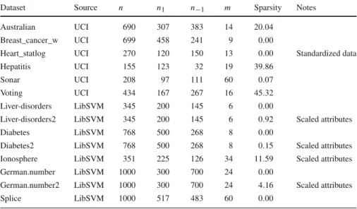
Table 2 Information on the 14 data sets used in the experiments
Dataset Source n n1 n−1 m Sparsity Notes
Australian UCI 690 307 383 14 20.04
Breast_cancer_w UCI 699 458 241 9 0.00
Heart_statlog UCI 270 120 150 13 0.00 Standardized data
Hepatitis UCI 155 123 32 19 39.86
Sonar UCI 208 97 111 60 0.07
Voting UCI 434 167 267 16 45.32
Liver-disorders LibSVM 345 200 145 6 0.00
Liver-disorders2 LibSVM 345 200 145 6 0.92 Scaled attributes
Diabetes LibSVM 768 500 268 8 0.00
Diabetes2 LibSVM 768 500 268 8 0.15 Scaled attributes
Ionosphere LibSVM 351 225 126 34 11.59 Scaled attributes
German.number LibSVM 1000 300 700 24 0.00
German.number2 LibSVM 1000 300 700 24 4.16 Scaled attributes
Splice LibSVM 1000 517 483 60 0.00
n1and n−1are the number of observations with yi =1 and yi = −1, respectively. Sparsity equals the percentage of zeros in the data set. A data set with scaled attributes has maximum values+1 and minimum values−1
To answer these questions, we consider the following measures. First, we define convergence between two steps as the relative decrease in loss between two subsequent steps, that is, by Ldiff = (Lt−1−Lt)/Lt. The error rate in the training data set is
defined as the number of misclassified cases. To measure how well a solution predicts, we define the accuracy as the percentage correctly predicted out-of-sample cases in fivefold cross validation.
6.1 Predictive performance for the three hinge errors
It is interesting to compare the performance of the three hinge loss functions. Con-sider Table 3, which compares the fivefold cross-validation accuracy for the three different loss function. For each data set, we tried a grid of λvalues (λ = 2p for
p = −15,−14.5,−14, . . . ,7.5,8 where 2−15 = 0.000030518 and 28 = 256).
Alongside are given the values of the optimal λ’s and times to convergence (stop whenever Ldiff<3×10⁻⁷). From the accuracy, we see that there is no one best loss function that is suitable for all data sets. The absolute hinge is best in 5 of the cases, the Huber hinge is best in 4 of the cases, and the quadratic hinge is best in 7 of the cases. The total number is greater than 14 due to equal accuracies. In terms of computational speed, the order invariably is: absolute hinge is the slowest, Huber hinge is faster, and the quadratic hinge is the fastest.
The implementation of optimal scaling regression was also done in MatLab, but the update in each iteration fory by monotone regression using the primary approach
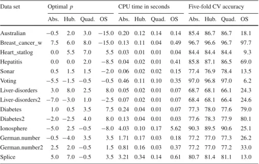
Table 3 Performance of SVM models for the three hinge loss functions (Abs., Hub., and Quad.) and
optimal scaling regression (OS)
Data set Optimal p CPU time in seconds Five-fold CV accuracy Abs. Hub. Quad. OS Abs. Hub. Quad. OS Abs. Hub. Quad. OS Australian −0.5 2.0 3.0 −15.0 0.20 0.12 0.14 0.14 85.4 86.7 86.7 18.1 Breast_cancer_w 7.5 6.0 8.0 −15.0 0.13 0.11 0.04 0.49 96.7 96.6 96.7 97.7 Heart_statlog 0.0 5.5 7.0 5.5 0.03 0.01 0.01 0.04 84.4 84.4 84.4 9.3 Hepatitis 0.0 0.0 2.0 −8.5 0.04 0.02 0.01 0.41 85.8 87.1 86.5 69.0 Sonar 0.5 1.5 1.5 −2.0 0.06 0.02 0.02 0.15 77.4 76.9 78.4 13.5 Voting −5.5 −1.5 −0.5 −0.5 0.46 0.11 0.10 0.35 97.0 96.8 97.0 6.2 Liver-disorders 3.0 8.0 2.5 8.0 0.05 0.02 0.01 0.07 68.7 68.1 66.1 24.3 Liver-disorders2 −7.0 −3.0 1.0 −2.5 0.07 0.02 0.01 0.07 68.4 68.1 66.4 24.6 Diabetes 1.0 0.5 3.5 7.5 0.24 0.04 0.01 0.07 77.3 78.0 77.6 79.0 Diabetes2 −2.0 −2.5 4.0 8.0 0.13 0.04 0.01 0.03 77.6 78.3 77.9 80.1 Ionosphere −5.0 2.5 −0.5 −8.0 4.03 0.10 0.17 5.62 90.3 89.5 90.6 25.1 German.number −0.5 −4.0 3.5 3.5 1.71 0.17 0.03 0.18 77.2 77.0 77.3 26.2 German.number2 2.5 2.0 −0.5 1.5 0.81 0.16 0.03 0.37 77.2 77.0 77.2 33.0 Splice 5.0 7.0 −0.5 3.5 3.21 0.34 0.14 0.61 80.7 81.4 81.1 13.0 The optimalλ=2pis computed by fivefold cross validation. CPU-time to convergence for the optimalλ and the prediction accuracy (in %) is obtained for the 14 different test data sets from Table2
not comparable to those of the other SVM methods that were solely programmed in MatLab. Optimal scaling regression performs well on three data sets (Breast cancer, Diabetes and Diabetes2) where the accuracy is better than the three SVM methods. On the remaining data sets, the accuracy is worse or much worse when compared to the SVM methods. It seems that in some cases OS regression can predict well, but its poor performance for the majority of the data sets makes it hard to use it as a standard method for the binary classification problem. One of the reasons for the poor performance could be due to solutions where allyˆis of one of the two classes collapses
in the inequality constraint and theyˆis of the other class remain to have variance. In
a transformation plot like Fig.3this situation means that the vertical scatter of either the−1 or 1 class collapses into a single point. By definition, the SVM transformation cannot suffer from this problem. More study is needed to understand if the collapse is the only reason for bad performance of OS-Reg, and, if possible, provide adaptations that make it work better for more data sets.
6.2 Computational efficiency of SVM-Maj
To see how computationally efficient the majorization algorithms are, two types of experiments were done. In the first experiment, the majorization algorithm is studied and tuned. In the second, the majorization algorithm SVM-Maj for the absolute hinge error is compared with several off-the-shelf programs that minimize the same loss function.
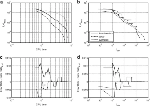
10-3 10-2 10-1 10-8 10-6 10-4 10-2 100 CPU time Lt -Lfinal 10-8 10-6 10-4 10-2 100 102 10-8 10-6 10-4 10-2 100 L diff Lt -Lfinal 10-3 10-2 10-1 -0.01 -0.005 0 0.005 0.01 0.015 CPU time
Error Rate - Error Rate
final 10-8 10-6 10-4 10-2 100 102 -0.01 -0.005 0 0.005 0.01 0.015 Ldiff
Error Rate - Error Rate
final liver disorders sonar australian a b c d
Fig. 6 The evolution of several statistics (see text for details) of three datasets: Australian (dotted lines),
Sonar (dash-dot lines), and Liver Disorders (scaled, solid lines). Values ofλ’s are fixed at optimal levels for each dataset. Loss function used: absolute hinge
As the majorization algorithm is guaranteed to improve the LSVM(c,w)in each iteration by taking a step closer to the final solution, the computational efficiency of SVM-Maj is determined by its stopping criterion. The iterations of SVM-Maj stop whenever Ldiff < . It is also known that majorization algorithms have a linear convergence rate (De Leeuw 1994), which can be slow especially for very small. Therefore, we study the relations between four measures as they change during the iterations: (a) the difference between present and final loss, Lt −Lfinal, (b) the
con-vergence Ldiff, (c) CPU time spent sofar, and (d) the difference between current and final within sample error rate.
Figure6shows the relationships between these measures for three exemplary data sets: Liver disorders, Sonar and Australian. Note that in Fig.6c, d the direction of the horizontal axis is reversed so that in all four panels the right side of the horizontal axis means more computational investment. Figure6a draws the relationship between CPU-time and Lt−Lfinal, with Lfinalthe objective function values obtained at convergence
with = 3×10⁻⁷. Notice that in most of the cases the first few iterations are responsible for the bulk of the decreases in the objective function values and most of the CPU time is spent to obtain small decreases in loss function values. Figure 6b shows the relationship between Lt−Lfinaland the convergence Ldiffthat is used as a stopping criterion. The two lower panels show the development of the within sample error rate and CPU time (Fig.6c) and convergence Ldiff(Fig.6d). To evaluate whether it is worthwhile using a looser stopping criterion, it is in instructive to observe
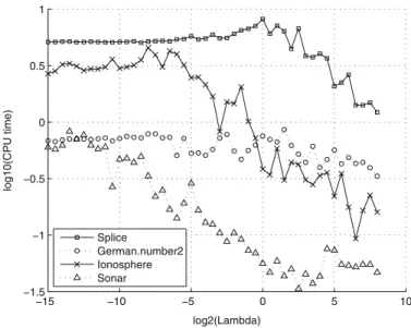
−15 −10 −5 0 5 10 −1.5 −1 −0.5 0 0.5 1 log2(Lambda) log10(CPU time) Splice German.number2 Ionosphere Sonar
Fig. 7 The effect of changingλon CPU time taken by SVM-Maj to converge. Loss function used: absolute hinge
the path of the error rate over the iterations (the lower right panel). It seems that the error rate stabilizes for values of Ldiff below 10−6. Nevertheless, late-time changes sometimes occur in other data sets. Therefore, it does not seem recommendable to stop the algorithm much earlier, hence our recommendation of using=3×10⁻⁷.
The analogues of Figs.6and7were also produced for the Huber hinge and quadratic hinge loss functions. Overall, the same patterns as for the absolute hinge function can be distinguished, with several differences: the objective function decreases much faster (relative to CPU time), and the error rate stabilizes already at slightly greater values for the convergence criterion. In addition, the number of iterations until convergence by and large decline (vis-a-vis the absolute hinge function).
Figure7investigates how sensitive the speed of SVM-Maj is relative to changes in the values ofλfor four illustrative datasets (Splice, German-number with scaled attributed, Ionosphere, and Sonar). As expected, the relationship appears to be decreas-ing. Thus, for large λ the penalty term dominates LSV M and SVM-Maj with the
absolute hinge does not need too many iterations to converge. Note that the same phe-nomenon is in general observed for the other SVM-solvers as well so that, apparently, the case for largeλis an easier problem to solve.
6.3 Comparing efficiency of SVM-Maj with absolute hinge
The efficiency of SVM-Maj can be compared with off-the-shelf programs for the absolute hinge error. As competitors of Maj, we use LibSVM, BSVM, SVM-Light, and SVM-Perf. Note that the BSVM loss function differs from the standard SVM loss function by additionally penalizing the intercept. Nevertheless, we keep BSVM in our comparison to compare its speed against the others. We use the same
14 data sets as before. As SVM-Maj, LibSVM, SVM-Light, and SVM-Perf minimize exactly the same loss function LSVMthey all should have the same global minimum. In addition to LSVM, the methods are compared on speed (CPU-time in seconds) at optimal levels of theλ=2p(or equivalent) parameter. Note that the optimal levels of λcould differ slightly between methods as the off-the-shelf programs perform their own grid search for determining the optimalλ, that could be slightly different from those reported in Table3. We note that the relationship between theλparameter in SVM-Maj and the C parameter in LibSVM and SVM-light is given byλ=0.5/C.
For SVM-Maj, we choose three stopping criteria, that is, the algorithm is stopped whenever Ldiffis respectively smaller than 10−4,10−5, and 10−6.
For some data sets, it was not possible to run the off-the-shelf programs, sometimes because the memory requirements were too large, sometimes because no convergence was obtained. Such problems occurred for three data sets with SVM-Perf and two data sets with SVM-Light. Table4shows the results. Especially for=10−6, SVM-Maj gives solutions that are close to the best minimum found. Generally, Lib-SVM and SVM-Light obtain the lowest LSVM. SVM-Maj performs well with = 10−6, but even better values can be obtained by a stronger convergence criterion. Even though the loss function is slightly different, BSVM finds proper minima but is not able to handle all data sets. In terms of speed SVM-Maj is faster than its competitors in almost all cases. Of course, a smallerincreases the CPU-time of SVM-Maj. Nevertheless, even for=0.0001 good solutions can be found in a short CPU-time.
These results are also summarized in Fig.8, where SVM-Maj is used with the default convergence criterion of =3×10⁻⁷. As far as speed is concerned (see Fig.8a), SVM-Maj ranks consistently amongst the fastest method. The quality of SVM-Maj is also consistently good as it has the same loss function as the global minimum with differences occurring less then 0.01. Note that SVM-Perf finds consistently much higher loss function values than SVM-Maj, LibSVM and SVM-Light. Generally, the best quality solutions are obtained by LibSVM and SVM-Light although they tend to use more CPU time reaching it.
7 Conclusions and discussion
We have discussed how linear SVM can be viewed as a the minimization of a robust error function with a regularization penalty. The regularization is needed to avoid overfitting in the case when the number of predictor variables increases. We provided a new majorization algorithm for the minimization of the primal SVM problem. This algorithm handles the standard absolute hinge error, the quadratic hinge error, and the newly proposed Huber hinge error. The latter hinge is smooth everywhere yet is linear for large errors. The majorizing algorithm has the advantage that it operates on the primal, is easy to program, and can easily be adapted for robust hinge errors. We also showed that optimal scaling regression has several features in common with SVMs. Numerical experiments on fourteen empirical data sets showed that there is no clear difference between the three hinge errors in terms of cross validated accuracy. The speed of SVM-Maj for the absolute hinge error is similar or compares favorably to the off-the-shelf programs for solving linear SVMs.
Ta b le 4 Comparisons between SVM solv ers: time to con v er g ence in CPU seconds and objecti v e v alues Dataset p T ime to con v er ge, in C PU seconds LSVM SVM-Maj Lib-BSVM SVM-SVM-Maj Lib-BSVM SVM-SVM Light Perf SVM Light Perf 10 − 4 10 − 5 10 − 6 10 − 4 10 − 5 10 − 6 Australian 0 0 .07 0 .08 0 .11 6395 . 27 0.30 76 . 80 − 202 . 67 202 . 69 202 . 66 220 . 81 203 . 17 202 . 07 − Breast_cancer_w 6 0 .03 0 .06 0 .10 0 . 06 0.18 0 . 09 0 . 89 58 . 21 58 . 05 58 . 02 58 . 03 205 . 03 58 . 03 205 . 03 Heart_statlog 0 0.02 0.02 0.02 0 . 08 0.14 0 . 10 1 . 43 91 . 50 91 . 49 91 . 49 91 . 48 91 . 52 91 . 48 91 . 52 Hepatitis 0 0 .01 0 .02 0 .03 0 . 05 0.09 0 . 06 62 . 14 46 . 31 46 . 29 46 . 28 46 . 28 48 . 43 46 . 28 48 . 43 Sonar 0 0.02 0.04 0.05 0 . 13 0.30 0 . 15 31 . 08 114 . 54 114 . 51 114 . 51 114 . 51 116 . 83 114 . 51 116 . 83 V o ting − 5 0 .06 0 .11 0 .11 0 . 09 0.13 0 . 12 5 . 15 26 . 46 25 . 76 25 . 76 25 . 76 25 . 76 25 . 76 25 . 76 Li v er -disorders 3 0.04 0.06 0.06 0 . 49 1.25 −− 248 . 56 248 . 43 248 . 42 248 . 42 253 . 03 −− Li v er -disorders2 − 6 0 .03 0 .04 0 .07 0 . 11 0.15 −− 249 . 67 249 . 62 249 . 59 249 . 59 249 . 63 −− Diabetes 1 0 .06 0 .09 0 .15 3 3 . 05 1.88 10 . 30 407 . 81 396 . 73 396 . 60 396 . 57 396 . 81 444 . 18 396 . 57 444 . 18 Diabetes2 − 2 0 .05 0 .07 0 .12 0 . 14 0.23 0 . 26 77 . 35 399 . 81 399 . 69 399 . 66 399 . 66 399 . 67 399 . 66 399 . 67 Ionosphere − 5 0 .12 0 .15 0 .38 0 . 24 0.67 0 . 88 233 . 19 55 . 63 55 . 51 55 . 33 55 . 32 56 . 56 55 . 32 56 . 56 German.number 0 0.13 0.35 0.55 15 . 21 0.54 1 . 87 87 . 73 522 . 37 521 . 94 521 . 89 521 . 88 524 . 33 521 . 88 524 . 33 German.number2 3 0 .14 0 .22 0 .38 0 . 27 0.39 0 . 23 82 . 49 539 . 51 539 . 44 539 . 40 539 . 39 539 . 63 539 . 39 539 . 63 Splice 5 0 .55 1 .01 1 .55 0 . 47 0.87 0 . 33 11 . 50 427 . 37 427 . 21 427 . 19 427 . 18 433 . 68 427 . 18 433 . 68 The v alues of λ = 2 p’s are fi x ed at le v els close to the optimal ones o f T able 3
Fig. 8 Difference in
performance of SVM algorithms with absolute hinge and SVM-Maj using=3×10⁻⁷.
a The CPU time used in seconds
and b the difference of L and the lowest L amongst the methods
10-2 100 102 104 Splice German.number2 German.number Ionosphere Diabetes2 Diabetes Liver-disorders2 Liver-disorders Voting Sonar Hepatitis Heart_statlog Breast_cancer_w Australian
CPU time in sec
10-10 10-5 100 105 Splice German.number2 German.number Ionosphere Diabetes2 Diabetes Liver-disorders2 Liver-disorders Voting Sonar Hepatitis Heart_statlog Breast_cancer_w Australian L - Llowest SVM-Maj LibSVM BSVM SVM-Light SVM-Perf a b
There are several open issues and possible extensions. First, the SVM-Maj algorithm is good for situations where the number of objects n is (much) larger than the number of variables m. The reason is that each iteration solves an(m+1)×(m+1)linear system. As m grows, each iteration becomes slower. Other majorization inequalities can be used to solve this problem yielding fast iterations at the cost of making (much) smaller steps in each iteration. A second limitation is the size of n. Eventually, when
n gets large, the iterations will become slow. The good thing about SVM-Maj is that
each iteration is guaranteed to improve the SVM-Loss. The bad thing is that at most linear convergence can be reached so that for large n one has to be satisfied with an approximate solution only. However, for m not too large and even reasonably large n, SVM-Maj should work fine and be competitive. The SVM-Maj for the quadratic and Huber hinge are computationally more efficient than the absolute hinge, so they result in a faster algorithm, even for reasonably large n.
Second, this paper has focussed on linear SVMs. Nonlinearity can be brought in in two ways. InGroenen et al. (2007), we proposed to use optimal scaling for the transformation of the predictor variables. Instead of using kernels, we propose to use I-splines to accommodate nonlinearity in the predictor space. The advantage of this approach is that it can be readily applied in any linear SVM algorithm. The standard way of introducing nonlinearity in SVMs is by using kernels. We believe that this is also possible for SVM-Maj and intend to study this possibility in future publications.
SVMs can be extended to problems with more than two classes in several ways. If the extension has error terms of the form f1(q)or f−1(q)then the present majorization results can be readily applied for an algorithm. We believe that applying majorization to SVMs is a fruitful idea that opens new applications and extensions to this area of research.
Open Access This article is distributed under the terms of the Creative Commons Attribution
Noncom-mercial License which permits any noncomNoncom-mercial use, distribution, and reproduction in any medium, provided the original author(s) and source are credited.
Appendix: Majorizing the hinge errors
Here we derive the quadratic majorizing functions for the three hinge functions.
A.1 Majorizing the absolute hinge error
Consider the term f−1(q)=max(0,q+1). For notational convenience, we drop the subscript i for the moment. The solid line in Fig.2a shows f−1(q). Because of its shape of a hinge, we have called this function the absolute hinge function. Let q be the known error q of the previous iteration. Then, a majorizing function for f−1(q) is given by g−1(q,q)at the supporting point q=2. We want g−1(q)to be quadratic so that it is of the form g−1(q) = a−1q2−2b−1q +c−1. To find a−1,b−1, and
c−1, we impose two supporting points, one at q and the other at−2−q. These two
supporting points are located symmetrically around−1. Note that the hinge function is linear at both supporting points, albeit with different gradients. Because g−1(q)is quadratic, the additional requirement that f−1(q) ≤ g−1(q)is satisfied if a−1 > 0 and the derivatives at the two supporting points of f−1(q)and g−1(q)are the same. More formally, the requirements are that
f−1(q)=g−1(q),
f−1(q)=g−1(q), f−1(−2−q)=g−1(−2−q),
f−1(−2−q)=g−1(−2−q), f−1(q)≤g−1(q). It can be verified that the choice of
a−1= 1 4|q+1| −1, (22) b−1= −a−1− 1 4, (23) c−1=a−1+ 1 +1|q+1|, (24)
satisfies all these requirements. Figure4a shows the majorizing function g−1(q)with supporting points q =1.5 as the dotted line.
For Class 1, a similar majorizing function can be found for f1(q)=max(0,1−q). However, in this case, we require equal function values and first derivative at q and at 2−q, that is, symmetric around 1. The requirements are
f1(q)=g1(q), f1(q)=g1(q), f1(2−q)=g1(2−q), f1(2−q)=g1(2−q), f1(q)≤g1(q). Choosing a1= 1 4|1−q| −1 (25) b1=a1+ 1 4 (26) c1=a1+ 1 2+ 1 4|1−q| (27)
satisfies these requirements. The functions f1(q)and g1(q)with supporting points
q =2 or q=0 are plotted in Fig.4a.
Note that a−1is not defined if q = −1. In that case, we choose a−1 as a small positive constantδthat is smaller than the convergence criterion(introduced later). Strictly speaking, the majorization requirements are violated. However, by choosing
δ small enough, the monotone convergence of the sequence of LSVM(w)will be no problem. The same holds for a1if q=1.
A.2 Majorizing the quadratic hinge error
The majorizing algorithm for the SVM with the quadratic hinge function is developed along the same lines as for the absolute hinge function. However, because of its struc-ture, each iteration boils down to a matrix multiplication of a fixed m×n matrix with
an n×1 vector that changes over the iterations. Therefore, the computation of the update is of order O(nm)which is more efficient than the majorizing algorithm for the absolute hinge error.
To majorize the term f−1(q) = max(0,q +1)2 is relatively easy. For q > −1,
f−1(q) coincides with(q +1)2. Therefore, if q > −1, (q +1)2 can be used to majorize max(0,q +1)2. Note that(q +1)2 ≥ 0 so that(q+1)2also satisfies the majorizing requirements for q < 1. For the case q ≤ −1, we want a majorizing function that has the same curvature as(q +1)2but touches at q, which is obtained by the majorizing function(q+1−(q+1))2=(q−q)2. Therefore, the majorizing
function g−1=a−1q2−2b−1q+c−1has coefficients a−1=1, (28) b−1= q if q≤ −1 −1 if q>−1 , (29) c−1= 1−2(q+1)+(q+1)2 if q≤ −1 1 if q>−1 . (30)
Similar reasoning can be held for f1(q) = max(0,1−q)2 which has majorizing function g1=a1q2−2b1q+c1and coefficients
a1=1, (31)
b1= 1 if q ≤1
q if q >1 , (32)
c1= 1 if q≤1
1−2(1−q)+(1−q)2 if q>1 . (33)
Again, ai,bi,and ciare defined as in (15), (16), and (17), except thatδin (15) can be
set to 0, so that ai =1=a for all i .
A.3 Majorizing the Huber hinge error
The majorizing algorithm of the Huber hinge error function shares a similar efficiency as for the quadratic hinge: the coefficients a1and a−1are the same for all i , so that again an update boils down to a matrix multiplication of a matrix of order m×n with
an n×1 vector.
To majorize h−1(q)we use the fact that the second derivative of h−1(q)is bounded. For q ≥ k, h−1(q)is linear with first derivative h−1(q) = 1, so that its second derivative h−1(q) = 0. For q ≤ −1, h−1(q) = 0, so that here too h−1(q) = 0. Therefore, h−1(q) >0 only exists for−1<q <k, where h−1(q)=1. Therefore, for −1 < q < k, the quadratic majorizing function is equal to h−1(q), for q ≤ −1 and q ≥ k, a quadratic majorizing function with the same second derivative of
(1/2)(k+1)−1is produced that touches at the current estimate q. Let the majorizing function g−1=a−1q2−2b−1q+c−1has coefficients
a−1=(1/2)(k+1)−1, (34) b−1= ⎧ ⎨ ⎩ a−1q if q ≤ −1 −a−1 if −1<q <k a−1q−1/2 if q ≥k , (35) c−1= ⎧ ⎨ ⎩ a−1q2 if q≤ −1 a−1 if −1<q <k 1−(k+1)/2+a q2 if q≥ −k . (36)
It may be verified for any q from the three intervals that h−1(q) = g−1(q) and
h−1(q)= g− 1(q)hold. In addition, g−1(q) =(1/2)(k+1)−1 ≥ h−1(q)for all q (as long as k >−1) so that the second derivative d−1(q)of the difference function
d−1(q)= g−1(q)−h−1(q)equals g−1(q)−h−1(q)≥ 0 indicating that d−1(q)is convex. As g−1(q)touches h−1(q)at q, d−1(q)=0, so that, combined with convexity of d−1(q)the inequality d−1(q)≥ 0 must hold implying the majorizing inequality
h−1(q)≤g−1(q)for all q with equality at q.
For h1(q)similar reasoning can be held. Let the majorizing function g1=a−1q2− 2b−1q+c−1has coefficients a1=(1/2)(k+1)−1, (37) b1= ⎧ ⎨ ⎩ 1/2+a1q if q ≤ −k a1 if −k<q<1 a1q if q ≥1 , (38) c1= ⎧ ⎨ ⎩ 1−(k+1)/2+a−1q2 if q ≤ −k a1 if −k<q <1 a1q2 if q ≥1 . (39)
Note that a−1and a1are exactly the same and both independent of q. Therefore, the curvature of the majorizing functions for all Huber hinge errors is the same. This property is exploited in the simple update derived from (22).
References
Borg I, Groenen PJF (2005) Modern multidimensional scaling: theory and applications, 2nd edn. Springer, New York
Burges CJC (1998) A tutorial on support vector machines for pattern recognition. Knowl Discov Data Min 2:121–167
Chang C-C, Lin C-J (2006) LIBSVM: a library for support vector machines (Software available athttp://
www.csie.ntu.edu.tw/~cjlin/libsvm)
Chu W, Keerthi S, Ong C (2003) Bayesian trigonometric support vector classifier. Neural Comput 15(9):2227–2254
Cristianini N, Shawe-Taylor J (2000) An introduction to support vector machines. Cambridge University Press, Cambridge
De Leeuw J (1994) Block relaxation algorithms in statistics. In: Bock H-H, Lenski W, Richter MM (eds) Information systems and data analysis. Springer, Berlin pp 308–324
Gifi A (1990) Nonlinear multivariate analysis. Wiley, Chichester
Groenen PJF, Nalbantov G, Bioch JC (2007) Nonlinear support vector machines through iterative majoriza-tion. In: Decker R, Lenz H-J (eds) Advances in data analysis. Springer, Berlin pp 149–162 Hastie T, Tibshirani R, Friedman J (2001) The elements of statistical learning. Springer, New York Heiser WJ (1995) Convergent computation by iterative majorization: theory and applications in
multidi-mensional data analysis. In: Krzanowski WJ (ed) Recent advances in descriptive multivariate analysis. Oxford University Press, Oxford pp 157–189
Hsu C-W, Lin C-J (2006) BSVM: bound-constrained support vector machines (Software available athttp://
www.csie.ntu.edu.tw/~cjlin/bsvm/index.html)
Huber PJ (1981) Robust statistics. Wiley, New York
Hunter DR, Lange K (2004) A tutorial on MM algorithms. Am Stat 39:30–37
Joachims T (1999) Making large-scale SVM learning practical. In: Schölkopf B, Burges C, Smola A (eds) Advances in kernel methods—support vector learning. MIT-Press, Cambridge (http://www-ai.