Comparative Analysis of Scattering and Random Features in Hyperspectral Image Classification

(1)

Procedia Computer Science 58 ( 2015 ) 307 – 314

Peer-review under responsibility of organizing committee of the Second International Symposium on Computer Vision and the Internet (VisionNet’15) doi: 10.1016/j.procs.2015.08.025

ScienceDirect

Second International Symposium on Computer Vision and the Internet

(VisionNet’15)

Comparative Analysis of Scattering and Random

Features in Hyperspectral Image Classification

Nikhila Haridas*, V Sowmya, Soman K P

Centre for Excellence in Computational Engineering and Networking, Amrita Vishwa Vidyapeetham, Amritanagar, Coimbatore-641112, India

Abstract

Hyperspectral images (HSI) contains extremely rich spectral and spatial information that offers great potential to discriminate between various land cover classes. The inherent high dimensionality and insufficient training samples in such images introduces Hughes phenomenon. In order to deal with this issue, several preprocessing techniques have been integrated in processing chain of HSI prior to classification. Supervised feature extraction is one such method which mitigates the curse of dimensionality induced by Hughes effect. In recent years, new strategies for feature extraction based on scattering transform and Random Kitchen Sink have been introduced, which can be used in context of hyperspectral image classification. This paper presents a comparative analysis of scattering and random features in hyperspectral image classification. The classification is performed using simple linear classifier such as Regularized Least Square (RLS) accessed through Grand Unified Regularized Least Squares (GURLS) library. The proposed approach is tested on two standard hyperspectral datasets namely, Salinas-A and Indian Pines subset scene captured by NASAs AVIRIS sensor (Airborne Visible Infrared Imaging Spectrometer). In order to show the effectiveness of proposed method, a comparative analysis is performed based on feature dimension, classification accuracy measures and computational time. From the comparative assessment, it is evident that classification using random features achieve excellent classification results with less computation time when compared with raw pixels(without feature extraction) and scattering features for both the datasets.

Peer-review under responsibility of organizing committee of the Second International Symposium on Computer Vision and the Internet (VisionNet’15).

Keywords: Classification; Feature Extraction; Hyperspectral; Random Kitchen Sink;Scattering transform

* Corresponding author. Tel.: +0-999-500-8969 E-mail address: [email protected]

Peer-review under responsibility of organizing committee of the Second International Symposium on Computer Vision and the Internet (VisionNet’15)

(2)

1.Introduction

The recent advance in sensor technology in the field of remote sensing has made it possible to capture images in a broad range of the electromagnetic spectrum, covering the visible and infrared region (0.4 to 2.5 μm). Hyperspectral sensors acquire data of a scene in hundreds to thousands of contiguous narrow spectral bands with high spectral and spatial resolution. Among the various hyperspectral image processing tasks, HSI classification has drawn much attention in recent years. The abundant spatial and spectral information present in hyperspectral images allows identification and discrimination of materials in the scene with great precision. However, the well-known difficulty in classification of hyperspectral images is Hughes phenomenon (curse of dimensionality) where, only limited training information is available for higher number of spectral channels. Moreover, the presence of redundant information and the increase in computational time due to high dimensionality may have a bad effect on HSI classification. Thus, the use of preprocessing techniques such as denoising, feature extraction, dimensionality reduction etc. has become an integral part of hyperspectral image classification systems.

In literature, a number of different approaches exist for preprocessing and feature extraction in HSI. Jiangfeng Bao et al. in1_{used spectral derivative features for classification of hyperspectral data. Other well- known techniques}

for preprocessing in hyperspectral imagery include Principal Component Analysis (PCA)2_{, Singular Value}

Decomposition (SVD) and Independent Component Analysis (ICA). Yuan Yan Tang et al. in3_{proposed three}

dimensional scattering wavelet transform which captures the spectral spatial information for HSI classification. Ali Rahimi et.al4_{introduced Random Kitchen Sink algorithm to significantly reduce the computation time needed for}

training kernel machines and for improving the classification accuracy. Inmaculada Dpido et al. in5_{performed a}

comparative study of different unmixing based feature extraction techniques for HSI classification. This paper presents the performance comparison of different feature extraction techniques in HSI classification. Three different features of hyperspectral images including raw pixels, scattering features and random features were considered for the assessment. The parameters used in the analysis of proposed work are feature dimension, classification accuracy and computational time. The study demonstrates that Random Kitchen Sink is a fast and efficient feature extraction mechanism which improves the performance of large scale HSI classification. Rest of the paper is outlined as follows. An overview of feature extraction techniques is given in section 2. A brief introduction to GURLS library is presented in section 3. Section 4 describes the methodology of the proposed work. Section 5 reports the experimental results and analysis and finally, section 6 concludes the paper.

2.Feature Extraction Techniques

This section gives a brief description about the conceptual basics of the feature extraction algorithms namely, Scattering Transform and Random Kitchen Sink.

2.1.Scattering Transform

An important characteristic required for features extracted for classification is that, they need to be translation invariant which do not affect the human ability to recognize. Apart from translation invariance, signal representation also need to be continuous with respect to transformations such as scaling or rotations and should contain enough information in order to discriminate between various signal classes. Scattering features6_{build informative signal}

representations through a nonlinear unitary transform which are stable and invariant with respect to small deformations. Scattering transform is therefore an efficient method to extract features based on the translational, rotational and convolutional invariance of image pixels. These informative invariant features are well adapted for image classification. The rich information present in hyperspectral image pixels is scattered along multiple paths implemented in a convolutional network architecture. A scattering vector is computed by cascading wavelet transform convolutions, modulus operators and local averaging. An open source software library called ScatNet is available for the computation of scattering vector.The detailed mathematical description of scattering operator is given by Bruna and Mallat6_{. Scattering Network output is given by,}

(3)

where ’x’ is the input pixel vector, ψ is the wavelet, φ is the scaling function and λ is the scale factor.

2.2.Random Kitchen Sink

Random Kitchen Sink is an efficient algorithm used to generate randomized features whose inner products approximate popular kernels4_{. The key idea behind the use of Random Kitchen Sink algorithm is that, it captures}

nonlinear properties of the data by mapping it to a high dimensional feature space probably an infinite dimensional space by using a mapping function, φ. Consider RBF kernel in defining Random Kitchen Sink algorithm. The expression for RBF kernel is given as

2 ₁

2 ( ) ( )

( , ) ( ) ( ) x y x yT x y z z ( )

k x y _{I I}x y eV eV e₆ k z (2)

where z = x −y i.e. the kernel function is completely dependent on the difference between two data points and

1_I

V

¦ is the covariance matrix and I is an N × N identity matrix with mean zero. This can be equivalently written in the form of 1 1 2 2 1 1 2 2 cos( ) cos( ) cos( ) cos( ) : : cos( ) cos( ) 1 1 ( ) , ( ), ( ) sin( ) sin( ) sin( ) sin( ) : : sin( ) sin( ) T T T T T T m m T T T T T T m m x y x y x y k x y x y m x m y x y x y I I ª : º ª : º « » « » : : « » « » « » « » « » « » « _: » « _: » « » « » | « : » « : » « » « » : : « » « » « » « » « » « » « _: » « _: » ¬ ¼ ¬ ¼ (3)

That is, each data point is mapped to cosines and sines to form a 2 m-tuple vector. Further, the inner product of the mapped data points is used to approximate the Gaussian kernel. The detailed mathematical description of RKS is given by Ali Rahimi et.al4.

3.GURLS- A Least Squares Library for Supervised Learning

Grand Unified Regularized Least Squares commonly known as GURLS is a software library used for supervised learning. The library is suited for multi-category/multi-label problems for machine learning tasks such as classification, regression etc. The fact that it reduces a learning problem into a simple linear algebraic problem makes it computationally efficient for learning tasks. GURLS library exploits the use of latest tools in linear algebra for generating solution7. The library is based on the Regularized Least Squares (RLS) which can easily handle large scale/high dimensional datasets which are difficult to manage for other linear learning methods. The favourable properties of RLS makes it an obvious choice as compared to many existing learning algorithms which go complicated when dealing with multi-classification problems.

Regularized Least Squares: RLS takes the input hyperspectral data and calculates the weight matrix W required for the classification. The objective function can be equivalently expressed in terms of the Frobenius norm of a matrix as, 2 2 min _F _F W WX Y OW (4) 1 1 2 1 2 3 ( ) ( ) ( ) ( ) ... x x t x t S x t x t O O O O O O I \ I \ \ I \ \ \ I § · ¨ ¸ ¨ ¸ ¨ ¸ ¨ ¸ ¨ ¸ ¨ ¸ ¨ ¸ ¨ ¸ © ¹ (1)

(4)

This expression is equivalent to

min (( )( ) )T ( T )

W tr WX Y WX Y tr W WO (5)

That is weight matrix W can be obtained as,

1 ( ) b b b b b b T T p n p N N n n N N n n n W Y X X X OI u u u u u u (6)

where X is the input hyperspectral data, Y is the label vector, p is the number of class and nb represents the number

of bands.

4.Methodology

Preprocessing : In this stage, the entire 3D hyperspectral cube, _X n n n1u u2 b_{is loaded for processing. Each image}

in HSI cube is of size n1un2 and contains total nb bands. Highly noisy bands in the HSI data are removed manually

in advance as they lack detailed information for land cover classification. For the ease of processing, the data is further represented in 2D form as_Xn Nbu _{where, N is the total number of pixels in the image. Each pixel vector}

i

x

belongs to nb_.

Feature Extraction: Scattering Transform and Random Kitchen Sink are the two feature extraction techniques used.

Scattering transform: Scattering features are extracted from the 2D hyperspectral image, X using ScatNet software package implemented in matlab. The scat function takes each pixel, xi for i = 1, 2, 3..., N as its input along with set

of linear operators corresponding to wavelet transforms. The informative signal representations of input data can be computed by varying the linear operators such as wavelet operators. Furthermore, scattering features can be generated by varying the filter types and its parameters. Morlet filter 2D is used in this experiment. The scattering coefficients are computed with a cascade of wavelet modulus operators and is implemented in a convolutional network architecture where the wavelet operator gives filter coefficients.

Random Kitchen Sink: Random features are generated using Random Kitchen Sink algorithm where the input hyperspectral data is mapped to a higher dimensional feature space i.e., each pixel vector xi is mapped to k

dimensional space where k!!nb by taking the sines and cosines of each pixel. When the data is projected to a

higher dimensional feature space, the data separability increases which helps in better classification.

Classification: The data points and labels for training and testing are generated from the extracted features and

ground truth information. Let the training data, training labels, testing data and predicted labels be represented by Xtr, Ytr, Xte and Yprrespectively. The weight matrix, Wis calculated from training data Xtr, and training labels, Ytr

according to the Eq. 6. With the calculated weight matrix, Wthe output class labels are predicted using the equation Ypr= WXte. The predicted labels are used for quantitative and qualitative assessment

5.Experimental Results

This section describes about the dataset, accuracy assessment measures and experimental results obtained by the proposed technique.

5.1.Dataset Description

The experiment is performed on the on two standard hyperspectral datasets namely, Salinas A and Indian Pines subset. Salinas A contains 86 x 83 pixels located within the Salinas scene at [samples, lines] = [591-676, 158-240]. The ground truth contains 6 classes which are mutually exclusive. A subset portion of the Indian Pines image, called the subset scene was also used to evaluate the performance of the proposed method. The subset is a part of 145 x 145 scene and contains pixels located within Indian pines scene at [27-94] [31-116]. The size of subset portion is 68 x 86 with 224 spectral channels. The subset scene contains 4 different classes with similar spectral signatures.

(5)

5.2. Accuracy Assessment Measures

In hyperspectral image classification, accuracy assessment is done both qualitatively and quantitatively. In qualitative assessment, a thematic map generated with the classification is considered to be accurate if it gives an unbiased representation of the ground truth image. Classification error in this case is the visual discrepancy between the generated thematic map and the reality. In order to quantify the accuracy assessment, a confusion matrix or error matrix is generated for the entire testing data. The classification accuracy measures such as Class wise Accuracy, Overall Accuracy, Average Accuracy and Kappa Coefficient may be derived from the confusion matrix9_.

5.3. Results and Discussion

This section presents comparative and quantitative assessment of different feature extraction methods in hyperspectral image classification. The study investigates the role of scattering (SF) and random features (RF) for improving the classification accuracy in HSI. In order to show the effectiveness of the feature extraction, raw pixels of hyperspectral image are also adopted for comparison. The analysis is based on the feature dimension, quantitative accuracy assessment measures and computational time.

5.3.1. Analysis of feature dimension

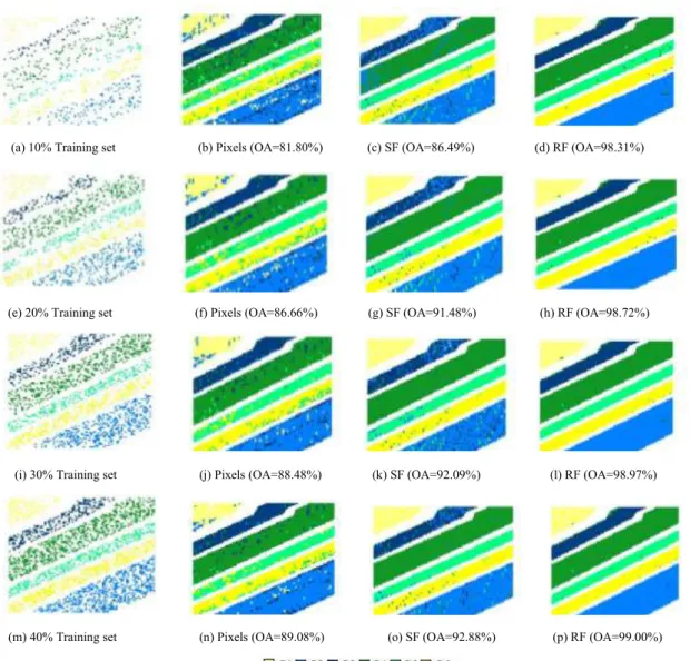
The role of feature dimension in increasing the classification accuracy is evaluated by empirically varying the number of input features given for classification. The training sets for the experiment are generated by randomly selecting samples from each class in equal ratio. The experiment is carried out on both the datasets with 10%, 20%, 30% and 40% training set. Fig. 1 and 2 shows the classification maps of the same. All the pixels other than the background pixels were used for validation. In the experiment with Salinas-A, a total of 5348 pixels were used to generate the training set excluding the background pixels. From the obtained results, it is clear that Salinas A produce excellent classification results for all the three input features even with 10% training set. The experiments with Indian pines subset scene demonstrates that better classification results are attained only with the larger training set (40%). This is because of the similarity in spectral signatures of various classes which leads to misclassification. The analysis of feature dimension shows that classification accuracy increases with the increase in feature dimensionality for both the datasets. Also, higher classification accuracies are obtained for Salinas A with limited number of training samples.

5.3.2. Analysis of accuracy assessment results

Based on the aforementioned training sets, quantitative assessment measures such as Overall Accuracy (OA), Classwise Accuracy (CA), Average Accuracy (AA) and Kappa Coefficient (K) were computed for both the data sets. Classification maps were also generated in each case for qualitative assessment. In order to assure statistical stability, the average classification results of three runs are given. Table 1 and 2 shows the comparison of land cover classification results of Salinas-A and Indian pines subset with 10%, 20%, 30% and 40% training set. It is worth noting that, CA, OA, AA and K of random features dominates for both datasets compared to other feature extraction approaches. Even though Salinas A produce satisfactory results without feature extraction (OA=81.80%, AA=81.95% and K = 0.7753), use of scattering and random features surpass the results produced by raw pixels. In the case of Indian pines subset scene, significant improvement in classification accuracy is obtained after incorporating feature extraction i.e for 40% training set OA improved from 61.78% to 74.92% and 93.34% by using scattering and random features. Despite the fact that scattering features improves the classification accuracy when compared to pixel features, they are computationally complex and time consuming. In comparison with raw pixels, the increments in OA for Salinas A dataset with limited training set (10%) of scattering and random features are 4.69% and 16.51% respectively and in the case Indian pines subset scene, OA shows significant increment of 19.6% and 41.22% for scattering and random features respectively.

(6)

`

Fig. 1: Training set, Classification map (without feature extraction (Pixels), Scattering Features (SF), Random Features(RF)) of Salinas A scene. C1, C2, C3, C4, C5, C6 represents the corresponding class numbers as given in Table 1.

Class name 10% 20% Percentage of training set 30% 40% Pixel SF RF Pixel SF RF Pixel SF RF Pixel SF RF 1 Brocoli green weeds 1 81.58 99.91 99.57 83.12 100 99.48 85.42 100 99.57 85.93 100 99.74 2 Corn senesced green

weeds 76.99 82.67 99.32 83.39 87.16 99.42 85.25 87.16 99.47 86.37 86.87 99.70 3 Lettuce_romaine_4wk 88.14 62.44 93.99 90.90 72.34 95.67 92.53 72.34 95.88 93.99 76.56 95.45 4 Lettuce_romaine_5wk 85.31 87.93 99.67 91.21 98.22 99.69 92.39 98.22 99.80 93.44 99.45 99.80 5 Lettuce_romaine_6wk 78.33 95.99 95.15 86.64 96.09 97.13 87.68 96.09 98.12 86.49 96.43 98.17 6 Lettuce_romaine_7wk 81.35 94.11 99.41 81.97 96.66 98.99 85.48 96.66 99.37 85.23 96.57 99.37 Overall Accuracy 81.80 86.49 98.31 86.66 91.48 98.72 88.48 92.09 98.97 89.08 92.88 99.00 Average Accuracy 81.95 87.18 97.85 86.21 91.42 98.40 88.12 90.43 98.70 88.57 92.65 98.70 Kappa Coefficient 0.775 0.830 0.978 0.834 0.893 0.983 0.856 0.900 0.987 0.864 0.910 0.987

(m) 40% Training set (n) Pixels (OA=89.08%) (o) SF (OA=92.88%) (p) RF (OA=99.00%) (a) 10% Training set (b) Pixels (OA=81.80%) (c) SF (OA=86.49%) (d) RF (OA=98.31%)

(e) 20% Training set (f) Pixels (OA=86.66%) (g) SF (OA=91.48%) (h) RF (OA=98.72%)

(i) 30% Training set (j) Pixels (OA=88.48%) (k) SF (OA=92.09%) (l) RF (OA=98.97%)

(7)

No Class name 10% 20% Percentage of training set 30% 40%

Pixels SF RF Pixels SF RF Pixels SF RF Pixels SF RF

1 Corn notill 36.81 67.33 80.59 44.37 51.64 85.24 46.16 51.54 87.19 45.27 47.06 87.82 2 Grass trees 57.12 99.26 97.48 70.95 99.63 97.67 74.79 99.90 99.26 75.20 100 99.40 3 Soybean notill 52.73 69.89 86.29 61.33 67.80 88.88 67.21 70.08 89.52 70.90 70.62 91.53 4 Soybean mintill 49.44 84.88 92.59 56.69 73.02 93.90 58.17 79.52 93.67 61.84 81.67 94.62 Overall Accuracy 48.37 67.97 89.59 57.02 71.67 91.70 59.70 74.91 92.42 61.78 74.92 93.34 Average Accuracy 32.68 69.87 89.24 38.89 73.02 91.42 41.05 75.26 92.41 42.20 74.84 93.34 Kappa Coefficent 0.328 0.548 0.850 0.428 0.597 0.880 0.463 0.639 0.891 0.489 0.730 0.904 (e) 20% Training set (f) Pixels (OA=57.02%) (g) SF (OA=71.67%) (h) RF (OA=91.70%)

(i) 30% Training set (j) Pixels (OA=59.70%) (k) SF (OA=74.91%) (l) RF (OA=92.42%)

(m) 40% Training set (n) Pixels (OA=61.78%) (o) SF (OA=74.92%) (p) RF (OA=93.34%) (a) 10% Training set (b) Pixels (OA=48.37%) (c) SF (OA=67.97%) (d) RF (OA=89.59%)

Fig. 2: Training set, Classification map (without feature extraction (Pixels), Scattering Features(SF), Random Features(RF)) of Indian Pines subset scene. C1, C2, C3, C4 represents the corresponding class numbers as given in Table 2.

(8)

5.3.3. Analysis of computation time

This section describes about the computation time required by each method for both the data sets. The experiment is performed on Intel(R) Core(TM) i7-4790S CPU, 8.00 GB memory, and 64 bit OS using MATLAB 2013. The running time includes the time required for feature extraction and classification. Table 3 shows the time analysis of raw pixels, scattering features and random features and Fig 3.shows the time analysis plot for classification of Salinas A. Among the three methods, random features (RF) have faster prediction time. The analysis clearly shows that scattering features (SF) are highly time consuming compared to raw pixels and random features.

6.Conclusion

This paper presents comparative analysis of feature extraction techniques such as scattering transform and Random Kitchen Sink for supervised land cover classification in hyperspectral images. In the experiment, we propose the benefit of feature extraction for improving the classification accuracy of remotely sensed hyperspectral data. The study demonstrates that scattering and random features accelerates the performance of simple linear classifiers such as Regularized Least Squares. Among the three methods( raw pixels, scattering transform and Random Kitchen Sink) used for comparison, random features proved to be efficient and powerful feature extraction technique with less computation time and excellent classification results. The scattering transform is observed to be computationally complex and time consuming method for feature extraction for high dimensional classification. As future work, the feature extraction techniques such as scattering transform can be implemented in GPU to save the processing time.

References

1. J. Bao, M. Chi, and J. A. Benediktsson, “Spectral derivative features for classification of hyperspectral remote sensing images:

Experimental evaluation,” IEEE Journal of Selected Topics in Applied Earth Observations and Remote Sensing, vol. 6, no. 2, pp. 594–601, 2013”.

2. G. Chen and S.-E. Qian, “Denoising of hyperspectral imagery using principal component analysis and wavelet shrinkage,” IEEE Transactions on Geoscience and Remote Sensing, vol. 49, no. 3, pp. 973–980, 2011.

3. Y. Y. Tang, Y. Lu, and H. Yuan, “Hyperspectral image classification based on three-dimensional scattering wavelet transform,” 2015

4. A. Rahimi and B. Recht, “Random features for large-scale kernel machines,” in Advances in neural informationprocessing systems, 2007, pp. 1177–1184.

5. I. Dopido, A. Villa, A. Plaza, and P. Gamba, “A quantitative and comparative assessment of unmixing-based feature extraction techniques for

hyperspectral image classification,” Selected Topics in Applied Earth Observations andRemote Sensing, IEEE Journal of, vol. 5, no. 2, pp.

421–435, 2012.

6. J. Bruna and S. Mallat, “Classification with scattering operators,” arXiv preprint arXiv:1011.3023, 2010.

7. A. Tacchetti, P. Mallapragada, M. Santoro, and L. Rosasco, “Gurls: a toolbox for large scale multiclass learning,” in NIPS 2011 workshop on parallel and large-scale machine learning. http://cbcl. mit. edu/gurls, 2011.

8. J. Li, J. M. Bioucas-Dias, and A. Plaza, “Exploiting spatial information in semi-supervised hyperspectral image segmentation,” in

Hyperspectral Image and Signal Processing: Evolution in Remote Sensing (WHISPERS), 2nd_{Workshop on}_{, 2010, pp. 1}_–_4.

9 S. K. Kavitha Balakrishnan, Sowmya, “Spatial preprocessing for improved sparsity based hyperspectral image classification,” in International Journal of Engineering Research and Technology, vol. 1, no. 5. ESRSA, July 2012

Dataset Feature 10 Time(sec) for different % of training data 20 30 40 Salinas A Pixels 20.59 100.92 275.57 552.81 SF 1024.59 1235.24 1562.83 1713.62 RF 14.60 77.69 227.20 494.29 Indian Pines Pixels 18.78 71.36 128.26 240.35 SF 996.40 1162.33 1388.46 1420.25 RF 12.82 66.37 115.75 232.48

Table 3. Time analysis of feature extraction techniques

Fig 3 Time analysis plot of Salinas A 0 500 1000 1500 2000 10 20 30 40 Ti m e( se c)

Percentage of training set(%) Raw pixels

Scattering features Random features