Break-Even Volatility

(1)

Break-Even Volatility

Nicolas Mitoulis

A dissertation submitted to the Faculty of Commerce, University of Cape Town, in partial fulfilment of the requirements for the degree of Master of Philosophy.

July 26, 2019

MPhil in Mathematical Finance, University of Cape Town.

University

of

Cape

(2)

The copyright of this thesis vests in the author. No

quotation from it or information derived from it is to be

published without full acknowledgement of the source.

The thesis is to be used for private study or

non-commercial research purposes only.

Published by the University of Cape Town (UCT) in terms

of the non-exclusive license granted to UCT by the author.

University

of

Cape

(3)

Declaration

I declare that this dissertation is my own, unaided work. It is being submitted for the Degree of Master of Philosophy at the University of Cape Town. It has not been submitted before for any degree or examination at any other University.

(4)

Abstract

A profit or loss (P&L) of a dynamically hedged option depends on the implied volatility used to price the option and implement the hedges. Break-even volatil-ity is a method of solving for the volatilvolatil-ity which yields no profit or loss based on replicating the hedging procedure of an option on a historical share price time series. This dissertation investigates the traditional break-even volatility method on simulated data, how the break-even formula is derived and details the imple-mentation with reference to MATLAB. We extend the methodology to the Heston model by changing the reference model in the hedging process. Resultantly, the need to employ characteristic function pricing methods arises to calculate the Hes-ton model sensitivities. The break-even volatility solution is then found by means of an optimisation of the continuously delta hedgedP&Lover the Heston model parameters.

(5)

Acknowledgements

I would like to express my gratitude to my supervisors at the African Institute of Financial Markets and Risk Management, Professor David Taylor and Obeid Ma-homed, for their guidance throughout the MPhil degree. I would also like to thank Emlyn Flint for proposing the topic of this dissertation. Lastly, my appreciation is extended to my family and friends for all the support they have given me.

(6)

List of Figures

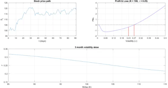
2.1 Three-month GBM price path with delta hedgedP&Lof a short call (K = 100) as a function ofσand corresponding break-even volatility skew. . . 4

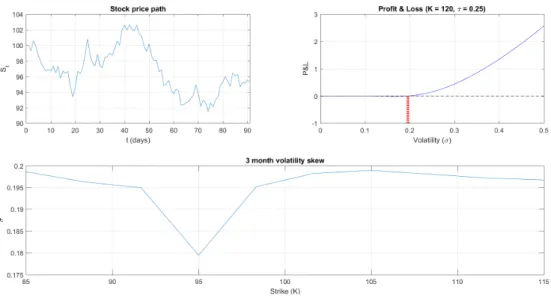
2.2 A GBM price path (with dynamics as in Section 2.1), a call option’s

P&Las function ofσand volatility skew plot. . . 11

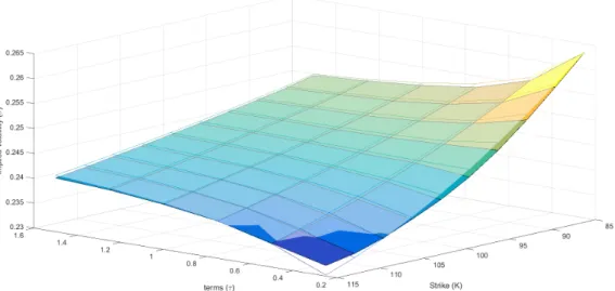
3.1 True implied volatility (transparent) and break-even volatility esti-mated surface (10 000 paths, MSE: 3.7873e-07). . . 17

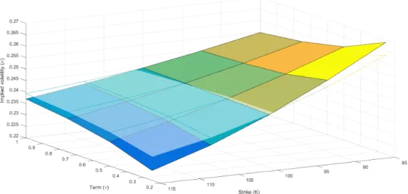
4.1 Optimising the whole surface: True implied volatility surface (trans-parent) and break-even volatility surface, averaged over all options (50 paths). MSE = 3.0074e-05. . . 21

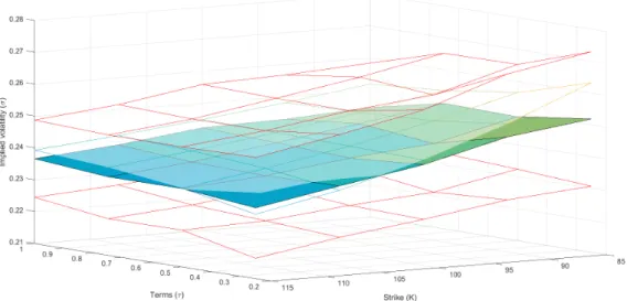
4.2 Point-wise optimisation: True implied volatility surface (transpar-ent) and break-even volatility surface, zeroing each path’sP&Lfor a specific option seperately (50 paths), in between 3 standard devia-tion bounds (red). MSE = 2.2235e-05. . . 22

4.3 Break-even volatility distributions for two options of 1-year term (sample size: 50). . . 23

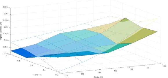
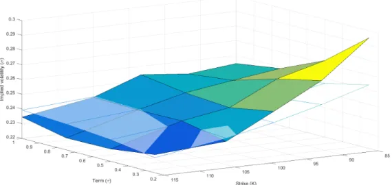
4.4 Point-wise optimisation: True implied volatility surface (transpar-ent) and point-wise optimised for Heston parameters, zeroing each options’ averageP&L(50 paths). MSE = 2.6976e-05. . . 25

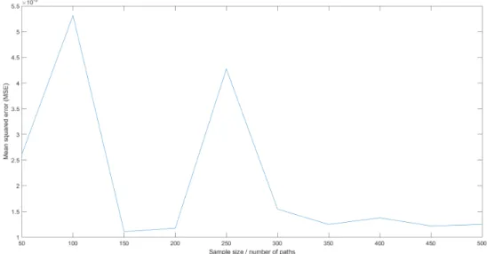
4.5 MSE as a function of sample size for the 3-month volatility skew, with strike price range 85% – 115% ofS0. . . 25

4.6 Optimising the whole surface: True implied volatility surface (trans-parent) and full surface optimised for Heston parameters, averaging all options’P&L’s (50 paths). MSE = 8.6556e-06. . . 27

4.7 True implied volatility surface (transparent) and point-wise optimised over Heston parameters (50 paths) using the realised variance in place of the actual variance path. MSE = 1.0397e-04. . . 28

(8)

List of Tables

4.1 Break-even volatility estimates for two options (50 sample paths). . . 23

4.2 Parameter estimates for 3-month skew with increasing sample size. . 26

(9)

Chapter 1 Introduction

Traditional option volatility estimation involves calculating the annualised stan-dard deviation of daily realised log returns from a historical time series of stock price data. This is only sensible in light of the constant volatility assumption of geometric Brownian motion (GBM). Naively, the realised volatility over a chosen period of time can be used in the Black-Scholes formula to yield a price, for any given strike or maturity. This ignores any market skew, where the implied volatil-ity (the volatilvolatil-ity input which equates the Black-Scholes option price to the market price) is not constant for options with different strikes and maturities on the same underlying.

A dynamically hedged option recoups the difference between realised volatility and the implied volatility, this is captured as either a profit or a loss. To do this, one must implement the correct hedge and an accurate method of estimating the option volatility. The traditional estimate of volatility gives no indication of how the market is actually pricing options on the underlying as it is not contingent on the option’s strike or maturity. This makes the differential between the implied and realised volatility difficult to discern.

Dupire (2006) presents a method using dynamic (delta) hedging to calculate break-even volatility (BEV) surfaces. He explains that this estimate is the fair volatil-ity to both sides of an option contract, as it is the volatilvolatil-ity which zeroes the option’s profit or loss. The paper highlights BEV surfaces as a tool to understand market volatility surfaces. Dupire assesses the level of evident mispricing and severity of market skews by comparing the implied volatilities to what the fair break-even volatility would have been over the option’s life. Subsequently, break-even volatil-ity has evolved from a historical analysis tool to become a volatilvolatil-ity estimation procedure, mostly for longer maturity options or where similar option information is unavailable.

It is difficult to obtain a realised volatility estimate for different strikes or matu-rities. This is precisely what the break-even volatility methodology aims to achieve.

(10)

Chapter 1. Introduction 2

It is shown in Section2.2from the calculation of BEV, any profit or loss arising dur-ing a dynamically hedged option is influenced by the option’s Gamma and is thus linked to strike and time to expiry. Solely based on past data, the methodology creates option specific, constant volatility estimates representing how the market should have been pricing and hedging if it were fair. Comparing these estimates with implied volatilities gives an indication of market sentiment and the degree of mispricing on an option.

The standard BEV methodology makes no assumptions about the data gen-erating process, it merely examines a time series of historical stock price data to produce an estimate of an option’s volatility. The method entails retrospectively delta hedging an option over a historical stock price path using the Black-Scholes model and solving for the volatility which makes the hedge a fair game. How-ever, if we have additional information about which type of process is generating the data, changing the reference model to match should in theory result in an im-proved hedge. With imim-proved replication of the profit/loss of the option, we would then find a better break-even estimate of the volatility used to price and hedge the option.

The stochastic volatility model ofHeston(1993) introduces an interesting exten-sion of the break-even volatility methodology. The standard method of break-even volatility is data intensive and typically employs statistical bootstrapping of his-torical stock returns to simulate more price time series and increase the data size. This cannot be done with a stochastic volatility process where the time series must stay unbroken to maintain the serial correlation structure. The Heston model is commonly used and makes for a challenging adaptation to the standard methodol-ogy due to its high parameter dimensionality and associated data problems for the break-even methodology.

Break-even volatilities are constant estimates for each option, much like im-plied volatilities, and do not provide a term-structure of volatilities. In essence, they serve as a base pricing platform. It is therefore important for an accurate ini-tial price/volatility to be estimated, by employing an appropriate reference model, not necessarily Black-Scholes. This dissertation reviews and examines the standard BEV methodology, providing notes of its implementation in MATLAB and high-lighting its shortcomings. In an attempt to improve BEV estimates, we analyse the effect of changing the reference model from Black-Scholes to Heston. This is done by a comparison of each method’s efficacy at returning the true implied volatility surface of the Heston process which generated the data.

(11)

Chapter 2 Break-Even Volatility

The former financial market model of choice has been the Black-Scholes model to calculate an initial option premium and subsequent hedges, where historical volatility has been used to determine the volatilityσ. Not only does this assume the future will be as volatile as the past, the constant volatility assumption neces-sitates that options on the same underlying will be priced with the same volatility. Due to many market models being used and in most cases when the assumption of constant volatility is violated, the historical volatility estimate would produce a premium unsuitable to the volatility risk and hedging cost.

The attempt to find an accurate price or volatility for an option leads to a more critical problem of finding what the fair volatility to both sides of the option con-tract should be, this would be the volatility which causes the option to break even.

Suzuki and Vyas(2011) note that in empirical tests (where the stock price process is known) using the historical volatility over the life of an option or even the market implied volatility at the time were insufficient in matching the total hedging costs without market friction. The report focuses on extending the break-even method-ology to incorporate transaction costs and other market conventions, as well as showing break-even volatility to be an efficient and fair pricing platform.

2.1 Basic methodology via discrete delta hedging

In his seminal paper on break-even volatility,Dupire(2006) formalised the method-ology as a means of finding the fair market volatility skew or surface. The volatility estimates which form the skew are solved for and equate the profit or loss (P&L) of a dynamically hedged option to zero.

This can be visualised in a toy example using a simulated GBM price path with dynamics

dSt= 0.08Stdt+ 0.2StdWt.

(12)

2.1 Basic methodology via discrete delta hedging 4

Fig. 2.1:Three-month GBM price path with delta hedgedP&Lof a short call (K = 100) as a function ofσand corresponding break-even volatility skew. sold a call option on the share with strikeK = 100and a term of three months. After performing a daily delta hedging experiment on this data until maturity using the Black-Scholes model and a chosen constant volatility, the hedge profit or loss then depends on the choice of volatility used to price and hedge the option. The solution which zeroes the hedge is the break-even volatility.

In Figure2.1the option expires deep in the money as seen in the top left three-month price path. By calculating theP&L as a function of the chosen volatility σ, we construct the graph on the top right of Figure 2.1. From the P&L graph, the break-even volatility is 0.27, which is considerably higher than the volatility used to simulate the data (0.2). The break-even estimate seems sensible due to the option expiring deep in the money, as such a volatile stock path requires the initial premium to be inflated as well as to calculate the necessary delta holdings in the stock. Even the historical volatility over the period of0.23is not sufficient to allow the hedge to break-even. Regardless of the level of moneyness, this historical estimate would have been the same and is thus a misleading estimate with which to price and hedge due to its inability to account for option specifics (strike and term). This lends weight to the use of break-even volatility estimates which in essence is a reweighting of the asset returns used in the historical estimate, where the weights depend on strike and maturity.

By finding the break-even volatility for different moneyness levels, one obtains a volatility skew all from this three-month price path. This skew is naturally highly dependent on the path used to create it and one could obtain an unrealistic view

(13)

2.2 Traditional BEV formula 5

of how an option should be priced by simply observing one price path. In Figure

2.1the stock price increases substantially within three months, lower strikes corre-spond to the option being deeper in the money and thus a higher premium must be charged to account for this as depicted in the skew.

This process can be repeated for different option maturities to create an entire volatility surface for a given asset. Results can then be smoothed by averaging over a number of historical periods. This can be done as follows:

1. Specify a strikeKand maturityτ, delta hedge (using Black-Scholes) an option daily over a period in history and compute theP&L(σ).

2. Find the break-even volatilityσK,τ such thatP&L(σK,τ) = 0.

3. Repeat 1 and 2 over all strikes and terms to create the volatility surface for that specific period.

4. Repeat above steps over all historical periods and average the results to arrive at the final break-even volatility surface.

By implementing the process above, a separate surface is created for each historical period which is useful to see prices or volatilities changing over time. This means one obtains a distribution of volatility surfaces from the individual distributions of break-even volatilities for each option. The break-even volatility surface is usually found by averaging the surfaces, alternatively for a single option the average break-even volatility would be the final estimate.

2.2 Traditional BEV formula

Discrete delta hedging a historical price path can be used to find break-even volatil-ities, however this method is not often used by practitioners. In this section, we show a method of deriving a formula for theP&Lwhich stems from a continuous delta hedging argument. In practice a discretised version of this formula is used to find break-even volatilities, where an integral is approximated with a summation.

2.2.1 Derivation

Suppose the true dynamics of an underlying stock price process are given by dSt=µtStdt+σtStdWt,

whereµt and σt are non-negative adapted/predictable processes. Since this is a general process that we assume for the stock and no assumptions are put on the

(14)

form ofµtandσt, break-even volatility is seen as a non-parametric volatility esti-mation procedure.

Assuming a constant risk-free rater, we sell and hedge a European option on the underlying using the Black-Scholes model with constant volatilityσ.

LetYt=C(t, St)be the Black-Scholes price process of this option. LetXtbe the value of the hedge portfolioΘ = (θ_t(0), θ_t(1)), consisting of the bank account growing at the risk-free rate and the stock, whereθ(1)_t = ∂C_∂S(t, St) = ∆t.

By accumulating the hedging errorZt := Xt−Ytto maturityT, we derive an approximate formula for the delta-hedged option’s profit/loss. To do this, we first need the dynamics of the hedge portfolio and of the Black-Scholes price.

Using

Xt=θ(0)_t ert+ ∆tSt =⇒ θ(0)_t =e−rt(Xt−∆tSt),

to ensure the portfolio is self-financing, the SDE for the hedge portfolio is dXt=θ_t(0)rertdt+θ(1)_t dSt

=r(Xt−∆tSt)dt+ ∆t(µtStdt+σtStdWt) = (rXt+ ∆t(µt−r)St)dt+ ∆tσtStdWt.

Using It ˆo’s lemma on the Black-Scholes price process and substituting the option price sensitivities for the standard Greek letters gives us

dYt=dC(t, St) = ∂C ∂t(t, St)dt+ ∂C ∂S(t, St)dSt+ 1 2 ∂2C ∂S2(t, St)d[S]t = Θtdt+ ∆t(µtStdt+σtStdWt) + 1 2Γtσ 2 tSt2dt = (Θt+ ∆tµtSt+ 1 2Γtσ 2 tSt2)dt+ ∆tσtStdWt.

NowC(t, St)satisfies the Black-Scholes PDE (shown in AppendixA.1) with con-stant volatilityσ and risk-free rater. The price sensitivities in the first term above are dictated by the pricing model (Black-Scholes in this case) and by substituting forΘtfrom the Black-Scholes PDE allowsdYtto be written as

dYt= (rYt+ ∆t(µt−r)St+ 1 2Γt(σ

2

t −σ2)St2)dt+ ∆tσtStdWt.

The expression fordZtis then found by eliminating the like terms indXtanddYt dZt=dXt−dYt=r(Xt−Yt)dt− 1 2Γt(σ 2 t −σ2)St2)dt =rZtdt+ 1 2ΓtS 2 t(σ2−σt2)dt.

(15)

Solving withe−rt as an integrating factor and integrating from 0–T, the P&L at maturity is obtained as e−rtdZt−re−rtZtdt= 1 2e −rt ΓtS2_t(σ2−σ_t2)dt Z T 0 d(e−rtZt) = Z T 0 1 2e −rt_Γ tS2t(σ2−σt2)dt ZT = 1 2 Z T 0 er(T−t)ΓtSt2(σ2−σt2)dt. (1) In the final step shown above, Z0 = 0due to the hedge portfolio being initially equal to the Black-Scholes price. Naturally the formula for theP&Lin Equation (1) is approximated by a daily sum using market stock price data. We can acquire the instantaneous varianceσ2_t with the relationship(dSt_St )2=σ2_tdtand obtain a formula for theP&Lin terms of the volatilityσused to price and hedge as

P&L(σ) = 1 2 N−1 X i=0 er(T−ti)ΓtiSti2 σ2∆ti− ∆Sti Sti 2! , (2)

wheretN =T is the maturity of the option,∆ti =δtare all equal daily increments and∆Sti =Sti+1−Sti.

A strength of the break-even methodology is it is non-parametric in nature, it makes no assumptions as to the true underlying stock price process. This is outright stated in the derivation of Equation (1), where we assume general stock dynamics and drift and volatility processes. By using the Black-Scholes model to price and hedge the option does not mean it is assumed the stock follows GBM, the Black-Scholes model acts as a converter in the same way the model is used to transform a price into an implied volatility.

To construct a volatility surface, one follows the same procedure as in the dis-crete hedging case and finds the volatility which zeroes Equation (2) for a specific option. This formula yields similar, if not slightly more stable, results than the discrete hedging method. Additionally, when concisely implemented, it is not as computationally expensive.

2.2.2 BEV as aΓ-weighted average

If we equate Equation (2) to zero and solve forσwe arrive at the following equation σ2δt= N−1 X i=0 wi ∆Sti Sti 2 , wherewi= er(T−ti)ΓtiSti2 PN−1 j=0 er(T−tj)ΓtjStj2 . (3)

We see that the break-even volatility is a weighted average of squared returns or realised variances. For a specific volatility i.e specific strike and term, the

(16)

aver-2.3 Implementation notes 8

age will be dominated by the returns where theΓt values are highest. This hap-pens for price changes close to the strike price and towards maturity of the option; these price changes have arguably the greatest effect on the outcome of the option. Thus, points on a break-even skew are averages of the same returns with differ-ent weights due toΓ’s dependence on the strike. The downside of this is that an average of break-even volatilities for a specific option term leads back to the histor-ical volatility for that period. Constructing the skew is then susceptible to sample variation because it depends on the chosen period. A different period is seen as a different sample and will result in a different estimate of the break-even volatility skew in the same way historical volatility changes for each period. This is to be considered when obtaining an estimate, however it is of little consequence as the method’s aim is to form an estimate of where the level of the market skew should have been.

2.3 Implementation notes

2.3.1 Fixed-point iteration

In Equation (3), theσfor which we are trying to solve is needed to calculate theΓti values. Thus if one chooses to find break-even volatility using this equation, then a fixed-point iterative algorithm (e.g. Newton’s method) is needed.

Likewise for Equation (2), an iterative algorithm is best for accuracy. In the interest of speed and if outright accuracy is not required (i.e. if the break-even volatility is a base estimate which will be adjusted), a simple grid search can be used to find the intercept region where theP&L is zero and interpolated to the desired accuracy.

2.3.2 Uniqueness of solution

In the implementation of the standard methodology, for complete accuracy, we use a combination of a grid search and MATLAB’s fzero function which employs the bisection method (amongst other iterative methods) to find the root of Equation (2).Dupire(2006) mentions that the root may not be unique, but a strictly positive root is guaranteed. We see this in Figure2.1where zero is also a solution. In some cases it appears that theP&Lis non-negative, such as in Figure2.2. This is due to machine precision where extremely small negative values of theP&Lfunction are returned as zero. A fine enough grid search is also not feasible as this becomes too computationally expensive when repeated for multiple options. To combat this, the MATLAB optimizer fmincon is used alongside the grid search and root finding

(17)

2.3 Implementation notes 9

algorithms, specifically for these occurrences. When a root cannot be found, the solution is then the largestσsuch that theP&Lis zero.

2.3.3 Aggregation of results

Time windows

Once a period in history is chosen for which the break-even volatility levels will be calculated, the next step is to subdivide this time series into smaller time windows with length corresponding to the term of the option. This presents another possi-bility as to whether these time windows are overlapping or not. The BEV method-ology provides more accurate and smoother results with a larger dataset, and over-lapping time windows might allow this. Consequently, the break-even volatilities for each time window will no longer be identically and independently distribution (i.i.d.) as they will be averages of the same squared returns. This would render the distribution of break-even volatilities misleading and may not be appropriate for finding interval bound estimates for the break-even volatility of an option.

In practice, it is common to use independent time series to find each break-even volatility estimate and assemble a distribution or average to obtain a final estimate. In doing this, one must either rebase the stock price at the beginning of each time series to a common value or alternatively work with relative option strike prices.

Another commonly used method of data aggregation involves both statistical bootstrapping and Monte Carlo simulation. One can convert a time series of share prices into a time series of returns

S={S0, S1, S2, . . . , SN} =⇒ R={r1, r2, r3, . . . , rN},

whereri = log(_SiSi₋₁)fori∈ {1,2, . . . , N}.

With sufficient evidence ofi.i.d.returns, one can randomly sample fromRand create a new time series of returns

R? ={r?₁, r?₂, . . . , r_M? },

where eachr?_i ∈RandM corresponds to the option term under consideration i.e. tM = T the option maturity. The time series of returnsR?is used to create a new sample path of share prices

S? ={S₀?, S₁?, S₂?, . . . , S_N?}, whereS₀?=S0andS_i?=S_i−1? exp(r_i?).

This can be repeated to create multiple sample paths, each with a break-even volatility. This is similar to bootstrapping where the initial sample size of the re-turns is increased and then Monte Carlo simulation is performed to the desired

(18)

2.3 Implementation notes 10

accuracy by repeatedly sampling returns to create share price paths to find break-even volatilities and the results averaged. Likewise, with the subdivision into inde-pendent time series, it is important to base the initial value of each generated path to a common value as we have done withS0above.

Averaging methods

When the break-even volatility is found for each independent period of history, a distribution of volatilities is created for a specific option from the accumulation of these estimates and the final estimate is the mean of the distribution.

Another method is to average the option’sP&L’s for all historical periods con-sidered and find the single volatility, which applies to all periods, that zeroes this average. In tests using simulated data, this method provides benefits in computa-tional efficiency, yields smoother surfaces and converges faster to the true implied volatility surface. The drawback of this method is that we will no longer have a distribution of break-even volatilities for each point on a skew/surface to provide a certain level of confidence in an estimate.

In finding a break-even volatility estimate, we would like this volatility to imply an option price such that the optionP&Lis zero on average. In simply averaging periodical break-even volatilities instead, we are zeroing eachP&Lbut with differ-ent volatilities all for the same option. Thus it makes sense to apply one volatility to all historical periods so that the averageP&Lis nil.

A reason why the latter method may be more desirable, we are forcing the dis-tribution of theP&L’s to be centred around zero for a given volatility. It seems that an outlying share price time series would have an associated break-even volatility which skews the volatility distribution more so than the correspondingP&L can influence the break-even volatility estimate which zeroes the averageP&L. This is especially evident in short maturities where a few large returns may dominate the weighted average in Equation (3) in finding the volatility, thus causing a radical estimate. Adding to this, large negative and positive P&L’s from different time periods may offset each other linearly in the average whereas these P&L’s may not translate linearly to their respective break-even volatilities so that the average volatility is equivalently balanced.

2.3.4 Caveats

As stated previously, machine precision may play a part in making the root finding more difficult and tedious, thus one must make use of a combination of algorithms to account for this. For instance, we noticed in a few cases theP&Lfunction

(19)

re-2.3 Implementation notes 11

peatedly returns slightly positive values before going back to zero, for increasing σ values. This is precisely what arises in theP&Lplot in Figure 2.2, causing ini-tial root finding to be incorrect. This may not occur often and is dependent on the volatility of the historical period, but is likely to occur when using many sample historical periods or bootstrap sampling more paths. This can cause inconsisten-cies in the break-even volatility surfaces, thus setting up the algorithm and stress testing with simulated data goes a long way.

Fig. 2.2:A GBM price path (with dynamics as in Section2.1), a call option’sP&L as function ofσand volatility skew plot.

There may be instability in break-even estimates for options with short maturi-ties, for strikes well outside of the price range of a given path and even for strikes which are well within or at-the-money (ATM) as seen in the volatility skew in Fig-ure2.2 for a strike of 95. Fortunately averaging over many time windows helps smooth this out but it contributes to slow convergence of shorter maturity options to the true implied volatility skew.

The next point is not necessarily a caveat, it is more as something to note. Noth-ing has been said of the issue of the risk-free rate. The correct daily rate along the time series of prices may be input each day in the hedging process, however we found that changes in the constant risk-free rate as high as 10% did not heavily impact break-even estimates and the volatility skews marginally change. This is in line with the findings ofDupire(2006) and he notes that the traditional historical estimate also disregards interest rates.

(20)

2.4 Shortcomings 12

2.4 Shortcomings

The break-even methodology is predominantly a pricing platform for instruments which trade on volatility and exotic or long-term options. It is also a means of gauging the volatility premium currently offered by the market. AsDupire(2006) notes, the aim is not to produce a term structure of volatilities which would aid in hedging, but rather an initial price.

The slow convergence and long run-times make this methodology difficult to work with and set up. One is forced to use a long time series of prices in order to have enough data to overcome instabilities in the break-even estimate. However, if a large dataset is used, these break-even volatility surfaces become static through time. If the historical period stretches too far into the past, the estimates would not be susceptible to frequent change as more data emerges and this could make it a troublesome pricing technique in a continually changing market.

A finite sample may be taken and bootstrapped in order to increase the size of the dataset and ensure smoother results. A problem with this, which we will see in the Heston model, is that by bootstrapping returns enforces these new prices to be log-normally distributed. This Monte Carlo style approach causes the volatility surface to flatten as in a Black-Scholes world (Dupire,2006) and converge to the realised volatility of the sample.

(21)

Chapter 3 Stochastic Volatility

Stochastic volatility (SV) models have been widely adopted in practice for their ability to produce similar volatility skews observed in the market. This is most notable for equity options which have negatively sloping volatility skews caused by share price returns being negatively correlated with volatility. This is known as the leverage effect and has been empirically observed byBakshi et al. (1997), amongst others.

SV models shed the restrictive constant volatility assumption in the Black-Scholes world and allow the volatility to vary through time as a stochastic process. Volatil-ity has also been observed to cluster, i.e. periods of large price changes yielding high realised volatility as well as periods of low volatility. The choice of model used in these periods dictates the pricing and hedging errors, and a model which as-sumes constant volatility would exacerbate these errors. To reduce this, the volatil-ity assumption must be continually changed to react to the market, however this causes disorganised changes in the hedge ratios (Gatheral, 2011, p. 2). The BEV methodology involves a constant volatility assumption for all the hedges, therefore it is reasonable to update the calculation with another choice of model.

3.1 The Heston stochastic volatility model

In this dissertation we examine the model ofHeston(1993) in our extension of the standard BEV methodology. The Heston model allows the stock price to be depen-dent on a time-varying variance process and produces skews and return distribu-tions consistent with those seen in the market.

(22)

3.1 The Heston stochastic volatility model 14

Model dynamics

For a stock priceStand variance processνtat timet, the dynamics of the Heston model are given by the following stochastic differential equations:

dSt=µStdt+√νtStdW_t(1) dνt=κ(θ−νt)dt+σ√νtdW_t(2), whereW_t(1),W_t(2)are correlated Brownian motions.

The parameters of the Heston model are given by: µ Expected/real-world rate of return.

κ Mean reversion rate. θ Long-term variance level.

σ Volatility of the variance process.

ρ Correlation parameter wheredW_t(1)dW_t(2)=ρdt.

As in the Black-Scholes case,µis the drift of the stock which is replaced byrin the risk-neutral world. The parameterκcontrols the rate of mean reversion of the variance to the long-term level ofνt, given byθ. The magnitude ofκwould deter-mine the length of time the volatility spends above or belowθ. This is consistent with the common observation of volatility tending to cluster for certain periods in the market. Intuitively, we must haveκ, θ >0for the process to be mean-reverting. These conditions ensure that the variance will revert to the long-term level, because the drift term fordνtwill be positive for periods of low volatility and likewise the variance will be dragged down whenvtis aboveθas there will be negative drift. The parameterρallows for correlation between the stock and variance processes, andσ determines the volatility of the latter process. These parameters control the height and skewness of the return distribution. With a negative correlation param-eter, the return distribution is skewed to the left. The fatter left tail means lower returns are more likely than higher returns, thus the option price for increasing strikes will decrease. This creates the negative volatility skew and explains the leverage effect.

The variance process is known as the square root process, introduced byCox et al.(1985), and is strictly positive if 2κθ > σ2 (known as the Feller condition), given the initial volatility is nonnegative i.e. it cannot become negative. Since the variance is a latent process where the level cannot be seen in the market, the initial varianceν0becomes another parameter of the model.

(23)

3.2 Monte Carlo experiment with standard BEV 15

Reasons for considering the Heston model for Break-even Volatility

There has not been any substantial research into the performance of the break-even volatility methodology on stochastic volatility data. The Heston model provides an assessment of the BEV methodology’s ability to recover the theoretically correct volatility skew.

The need to bootstrap sample share price returns to simulate new price time series is vital to the methodology in order to construct smooth and stable surfaces. This method is commonly used by practitioners, but can no longer be done with Heston simulated data or any market data which may follow a SV process. The cor-relation between price and volatility creates a serial corcor-relation structure amongst the daily prices and thus the day-to-day returns will also share this correlation. The inherent assumption that the daily returns arei.i.d. involved in bootstrapping the data and sampling daily returns to create new paths would destroy this correlation and lead to a flat volatility surface. The inability to do this in practice would leave one with limited data when looking for a recent market volatility skew. Alterna-tively, one could choose to use a large time series of prices with the drawback that the volatility surface will not be susceptible to change as more data emerges.

Dupire(2006) mentions that alternative models to Black-Scholes may be used in order to improve the replication/hedge and then these “volatilities”, which are pa-rameters from the alternative model, may be converted into Black-Scholes implied volatilities. We examine how the standard methodology performs on a simulated dataset without conducting bootstrap sampling to create more data. We compare this to using the Heston model option price sensitivities (Γin Equation (2)), which we hope will provide an improvement in the form of reduced estimation error and will somewhat overcome the sampling error involved with a small dataset.

3.2 Monte Carlo experiment with standard BEV

As a sanity check, we perform a Monte Carlo simulation experiment. This is to verify that, given enough data, the standard BEV methodology can recover the true volatility surface implied by a Heston model with specific parameters. This being possible, the mean squared error (MSE) would decrease by using the theoretically correct model in the hedging process. This is not unequivocally checked due to the amount of data in this simulation being computationally infeasible for calculating theP&Lwith the Heston model.

The following parameter set was used in this simulation experiment which will become the base scenario for the rest of this dissertation:

(24)

3.2 Monte Carlo experiment with standard BEV 16 • ν0= 0.06, • κ= 9, • θ= 0.06, • σ = 0.5, • ρ=−0.4.

We set S0 = 100 and hedge with risk-free rate r = 0.06. We let µ = 0.08 for the sake of simulating non-risk neutral price paths. This, however, makes minimal difference to the BEV estimates and we are interested solely in the listed parameters for pricing purposes whereµhas no impact.

Here we are performing a pure simulation experiment, therefore there is no need to consider subdivision of time series or bootstrapping daily returns, each path will be a complete and independent Heston price path simulated via a Mil-stein scheme (see AppendixA.2.1for this discretisation). We simulate 10 000 daily stock price paths of the longest maturity considered (1.5 years), where BEV esti-mates for shorter-dated options are based on the initial segment, with length cor-responding to the specific option, of each independent path. TheP&L’s are calcu-lated using Equation (2) and the method of averaging allP&L’s for each option is employed for its stability and computational advantages, so that each point on the surface is the volatility which zeroes the averageP&Lover 10 000 paths.

The volatility surface in Figure 3.1 is constructed for standard European op-tions where the maturities range from three months to 18 months, increasing in increments of three months. The strike price ranges from 85% to 115% of the spot priceS0= 100.

In practice this amount of data is not available, however when given enough data we see that calculating the break-even volatility can recover the true implied volatility surface fairly well. In Figure3.1, the MSE between the implied and break-even volatility surfaces is 3.7873e-07. Heston (1993) acknowledges that daily re-turns are asymptotically normally distributed as the variance process reaches a steady state distribution in the long run with mean θ, given the mean reversion parameterκ > 0(Coxet al.,1985). This explains why the standard methodology works well, with Heston simulated data, for options with longer maturities and is able to overcome the instabilities frequently observed when estimating break-even volatility for short-term options. This is evident in Figure3.1 where the MSE for the shortest skew is tenfold that of the MSE for the longest skew (1.2247e-06 and 1.8617e-07 respectively). This is a significant difference considering the sample size.

(25)

3.3 Proposed method using Heston Greeks 17

Fig. 3.1:True implied volatility (transparent) and break-even volatility estimated surface (10 000 paths, MSE: 3.7873e-07).

Monte Carlo option pricing typically relies on simulating a larger amount of data than used here, however the break-even method performs well regardless. If there is evidence that a certain stock follows a SV process or there is a degree of serial correlation in a share price, the amount of data used here would not be able. Even for the shorter term options where there is technically more data avail-able due to shorter independent time series needed, instabilities arise and estimates worsen. A 20-year time series of daily prices would provide only 80 three-month non-overlapping paths, and thus other methods must be explored to improve the approximation.

3.3 Proposed method using Heston Greeks

In an attempt to improve the replication of the option in the delta-hedging pro-cess, we change the reference model from Black-Scholes to the correct model from which the data is being sourced. The aim is to obtain a more accurate picture of the volatility skew than the standard methodology and to assess whether the potential reduction in error from changing the reference model is worthwhile. Apart from an implied volatility price, another output is the Heston parameters which imply this price. Thus we can obtain the model dynamics as an added bonus, somewhat of a pseudo calibration.

Changing the hedging and pricing model substantially alters the scale of the problem. In the case of the Heston model, we now need to zero theP&Lwhich

(26)

becomes a function of multiple parameters. This presents itself as an optimisation problem akin to market calibration of the Heston model, with accompanying diffi-culties. Furthermore, implementing a delta hedge using the Heston model requires the starting value of the variance process (ν0) to be known. In our case of dynamic hedging along a stock price path, the corresponding latent variance process needs to be known at each point in order to calculate theΓti values in Equation (2).

The proposed way forward is to simulate data using the Milstein discretisation, thus allowing the volatility path to be known, which is not the case in practice. This would allow us to see the extent to which a change in the reference model reduces estimation error when compared to the standard BEV methodology.

With theP&Lbecoming a function of the parameter set{κ, θ, σ, ρ}, instead of a single volatilityσ with Black-Scholes delta hedging, zeroing theP&Lbecomes an optimisation problem. The initial varianceν0 is usually a parameter of the Heston model, but since we are performing pure simulation and have access to the variance process, we treat this as known.

For a break-even estimate based on a single price path (St, with corresponding variance pathvt), the following procedure explains how the optimisation is carried out to zero theP&Lcalculated using the Heston model. The optimisation is scaled up over many historical periods similarly to the standard methodology by either averaging estimates for each period or zeroing the average P&L. For a specific optionP&L, this optimisation is outlined below:

1. For a given parameter set{κ, θ, σ, ρ}, price the option using the Heston model and convert this price into a Black-Scholes implied volatilityσwhich is used in Equation (2).

2. Calculate theP&Lfrom Equation (2) using the HestonΓti’s which rely on the Heston parameter set above and correspondingνtivalues.

3. Solve for the Heston parameters which zeroes theP&Lusing a global opti-misation algorithm.

4. Convert these optimal parameters into a Black-Scholes implied volatility, as in 1, to find the break-even volatility.

An initial guessx0 ={κ0, θ0, σ0, ρ0}must be set when performing the optimisa-tion. If an extensive global optimisation algorithm is used, the optimal parameters are fairly stable between different cycles of the optimisation. Different solutions may occur due to random scattering of test points from the initial guess involved in the global algorithm. Consequently, the optimisation avoids finding local min-ima solutions and an accurate initial guess is therefore not crucial. Alternatively if

(27)

a global algorithm is not used, the solution will depend onx0and will likely find a local minimum.

The break-even methodology requires theP&Lto be zeroed, one cannot simply minimise theP&Lfunction. The method used in this dissertation is to minimise the square of theP&Lfunction which will still allow a root to be found, should one exist as a function of the four Heston parameters, and maintain differentiability.

The optimisation is carried out on steps 1 and 2 above. The option needs to be priced in each iteration of the optimisation to yield an implied volatility from the parameters which is used in Equation (2). This appears asσ2in the equation.

Utilising this method involves characteristic function pricing methods where integrals need to be approximated to price and find the Greeks under the Heston model. We use the Little Heston Trap formulation (seeA.2.2) in our optimisation. This specification of the characteristic function is used to calculate the Γ for the Heston model (seeA.2.3) as well as to find the Heston price implied volatility (σ2 in Equation (2)) from the Heston parameters being optimised. Separate from the optimisation procedure, the Heston price is calculated again in step 4 using the optimal Heston parameters and this price is converted into the final break-even volatility implied by the Heston model.

The variance process is simulated alongside the stock price process, rendering this investigation as a purely theoretical study. We simulate data using the Milstein discretisation with the same parameters as in Section3.2, however with far fewer sample paths, and compare the standard method to the method described above. Following this, using the same data, we use the realised variance(∆St_St )2as a proxy in place of the actual variance processνtand assess its viability as a substitute. This eliminates the need to have calibrated daily to uncoverνtcorresponding to a stock (given there is sufficient stability of the calibrated parameters), which can be used in the method above.

This method requires past price data only and may prove useful when no op-tion informaop-tion is available on the specific stock in order to calibrate the model to prices. However, if the model has been calibrated over time, then there will be a time series of daily parameters which can be used to obtain estimates of implied prices for options. These parameters only minimise the model pricing error to past observed prices and there is no implication that these would give true fair prices, which break-even volatility aims to do.

(28)

Chapter 4 Implementation and Results

In this section we construct BEV surfaces, initially using the Black-Scholes model to hedge, and then implement the methodology using the Heston model as the new reference model. The data is also sourced from the Heston model and the volatility surfaces are assessed by their MSE’s. The intention is to see whether the change in reference model from the standard methodology improves estimation of the true implied volatility surface.

This is done with simulating Heston stock price paths with the same parame-ters as in Section3.2. Both methods are computationally expensive, however the optimisation required when hedging with the Heston model slows the break-even method down even further and the usage of large datasets becomes infeasible. Therefore, only 50 independent paths are used for each method. We also only con-sider one-year options in order to limit the data size needed. Using fewer paths links to the fact that practitioners would not be able to bootstrap the data and cre-ate more paths, since this would break the covariance structure of the time series. Using 50 independent three-month stock price paths equates to a 12.5 year unbro-ken time series, this appears to be in the middle ground for amount of historical data. Any longer than this, there is a risk of static surfaces not changing over time and any shorter would not allow enough data. Naturally, for the one-year option, 50 independent one-year paths would not be readily available in most cases. To overcome this and have more sample paths, a practitioner may use paths which overlap. In doing this, it maintains the completeness of a path. However, if one is trying to obtain a distribution of break-even volatilities with the standard method-ology (as in Section2.1and2.3.3) then these volatility estimates for each path will no longer bei.i.d.. Applying overlapping time series means that a number of share price returns from one time series which form part of the weighted average of one break-even volatility estimate will be used in another estimate. The effect of which is not investigated in this dissertation and may not make a significant difference de-pending on the degree of overlapping. We choose to focus on using independent

(29)

4.1 Standard BEV 21

time series for each break-even estimate.

4.1 Standard BEV

Here we see how the standard method performs on few sample paths. If we think of break-even volatility in the context of Monte Carlo, the more sample paths used, the closer the result will be to the true solution. We saw this in our Monte Carlo experiment in Figure3.1that, given enough sample paths, break-even volatility can recover the true implied volatility surface.

Fig. 4.1:Optimising the whole surface: True implied volatility surface (transpar-ent) and break-even volatility surface, averaged over all options (50 paths). MSE = 3.0074e-05.

The result of using only 50 paths can be seen in Figure4.1, where the average P&L for all options on the surface is zeroed. The common method is to calcu-late and zero the average P&L for one option over many time series. Here we have modified this approach and averaged all options’P&Ls over all of the time series. In tests between finding the whole surface at once versus for each option separately, there were significant decreases in computational time using the former method. However, averaging all options’P&Ls and zeroing this average does not necessarily imply that each option’s averageP&Lis zeroed. In fact, not having this requirement yields an inaccurate representation of the volatility surface as different option’sP&Ls can offset each other in this average and result in wildly inaccurate break-even volatility estimates. In our implementation, the MATLAB minimiser fmincon is used where the input variable is the whole volatility surface/matrix.

(30)

4.1 Standard BEV 22

Each element of the matrix represented a break-even volatility for the correspond-ing option on the surface. The volatilities are used to calculate each option’s av-erageP&Lover the 50 time series and then the whole surface P&L is averaged. A non-linear condition was added onto the optimisation to ensure each option’s averageP&L was zeroed and the minimisation was carried out on the square of the averageP&Lof the whole surface to ensure differentiability in finding the root of this function. In turn, this leads to the same solution as if you were to construct the volatility surface with each option individually by zeroing the averageP&L, although with advantageous computing time.

For comparison we have added Figure 4.2 where the break-even volatility is found for each path and each option, producing a distribution of volatilities. The surface is well behaved and lies within the three standard deviation bounds. In most cases we find that zeroing the averageP&L produces smoother results and improves convergence to the true result. However, the MSE of4.2is similar in scale to that of Figure4.1, with the added benefit of having a certain degree of confidence in the estimate due to the resultant distribution.

Fig. 4.2:Point-wise optimisation: True implied volatility surface (transparent) and break-even volatility surface, zeroing each path’sP&Lfor a specific option seperately (50 paths), in between 3 standard deviation bounds (red). MSE = 2.2235e-05.

In Figure4.3, the break-even volatility distributions for two options (one-year term, strikes of 85 and 100) have been included as an example of what one would obtain by calculating the break-even volatility for each sample path. The final BEV estimates are either the means of the distributions or the volatilities which zero

(31)

4.2 Optimising over Heston parameters 23

the average P&L’s, the latter method being more accurate as seen in Table 4.1. With such few sample paths, the estimates in Table4.1are slightly lower than the true implied volatility as expected. The distributions suffer from significant sample variation due to the small sample size, this is evident from the instabilities and mul-tiple peaks. However, we do obtain accurate confidence intervals (Figure4.2) with the distributions being seemingly symmetrical. This makes the method of finding the distribution more attractive, as the highly volatile paths will be quantified as an outlying volatility in the distribution.

Fig. 4.3:Break-even volatility distributions for two options of 1-year term (sample size: 50).

(K = 85,τ = 1) (K= 100,τ = 1) True implied volatility 0.2517 0.2447

Zero averageP&L 0.2461 0.2424

Distribution mean 0.2444 0.2422

Tab. 4.1:Break-even volatility estimates for two options (50 sample paths).

4.2 Optimising over Heston parameters

In initial tests, point-wise estimation of break-even volatilities is performed. This means that the surface is constructed option-by-option and the Heston parameters, which imply the break-even volatility, were found by zeroing the averageP&Lof all sample paths. SinceΓandσ2in Equation (2) are now functions of the parameter

(32)

set{κ, θ, σ, ρ}, we need to calculate these by approximating the integrals in

charac-teristic function pricing. This is done by mid-point quadrature shown in Appendix

A.2.2to calculate the Heston price implied volatilityσ and the HestonΓinA.2.3. To implement the break-even method using Heston parameters, one needs to find the correspondingΓvalues along a price and volatility path, this involves a sum-mation to approximate the integral at each point along a time series. Following this, the sum needs to be taken over each path to find the associatedP&Land then averaged over all the paths. The most effective implementation of this involves some nifty matrix manipulation and multiplication in MATLAB which will sub-stantially speed up computational time and be useful when optimising over the full implied volatility surface. In our case, we simulate data where each stock path forms a row of the data matrix. We then expand into three dimensions to perform the quadrature at each point along a path.

The optimisation presents difficulties in that it is now similar to the problem of market calibration of the Heston model where an objective function needs to be minimised over the parameters as well. In calibration of the Heston model, different parameter sets can yield the same value of the objective function giving evidence that it, and theP&Lfunction under consideration, is flat at the minimum (Cui et al., 2017). In our case, different combinations of the Heston parameters can be returned as solutions which minimise theP&L. The optimal solution may depend on the optimisation algorithm and several sets of solutions may be found due to different starting points leading to local minima. Fortunately, we have found that various parameter sets all which minimise theP&Lclose to zero yield the same implied volatility around the correct level. This method is able to pick up the shape of the skew, however the optimal parameters may not the true parameters which simulated the data.

The parameter set{κ, θ, σ, ρ}solution is sensitive to the starting point chosen. To circumvent long run times, the function fmincon is used with the starting point as the true solution{κ, θ, σ, ρ}={9,0.06,0.5,−0.4}. In cases where no information is available to choose an appropriate initial point, a global optimisation algorithm (e.g. gs in MATLAB) can be used with similar effect.

The result of this point-wise optimisation can be seen in Figure4.4 where the MSE is similar in scale to those of the standard method in Figures 4.1 and 4.2. We know that implementing the theoretically correct hedge, by using the Hes-ton Greeks, should yield a more accurate implied volatility solution and converge quicker with more data. With the small sample size, we can only note that a change in the reference model works just as well.

(33)

Fig. 4.4:Point-wise optimisation: True implied volatility surface (transparent) and point-wise optimised for Heston parameters, zeroing each options’ aver-ageP&L(50 paths). MSE = 2.6976e-05.

squaredP&Lis close to zero, since this is the function being minimised. In Figure

4.5, the MSE is calculated for the 3-month skew with increasing sample size, where the data is simulated with the same parameters as before. Taking the implemen-tation a step further, the whole skew is optimised to give one parameter set, not as before by calculating theP&L option by option. After some large variations,

Fig. 4.5:MSE as a function of sample size for the 3-month volatility skew, with strike price range 85% – 115% ofS0.

(34)

the MSE appears to decrease and flatten out with no further improvement and the parameter estimates in Table4.2paints the same picture.

Parameters Sample size (number of paths) True values

100 200 300 400 500

κ 8.9885 8.9938 8.9934 8.9941 8.9930 9 θ 0.0552 0.0596 0.0591 0.0589 0.0606 0.06 σ 0.5185 0.5173 0.5195 0.5157 0.5186 0.5 ρ -0.5111 -0.5042 -0.5129 -0.5039 -0.5114 -0.4

Tab. 4.2:Parameter estimates for 3-month skew with increasing sample size. It appears that the estimates forκ,θandσ are close to the true values, but ad-mittedly the success of this estimation highly depends on the choice of parameters used to simulate and the interval bounds used in the minimisation algorithm of theP&L. Restricting the bounds for ρ to be between [−1,0], which fits for most equity option prices, allows for more accurate estimates as seen in Table4.2, other-wise with[−1,1]bounds forρthe estimates are even further astray. The parameter θcan be estimated with the most confidence, regardless of the interval bounds or the chosen true value used in the simulation. This is the least we could hope for as the implied volatilities can be somewhat approximated using the Heston model as seen in Figure4.4. The long-term varianceθcontrols the vertical position of the volatility surface and since this method can recover these average volatility levels as well as the approximate shape of the skew, it makes sense thatθcan be reliably estimated.

Analogous to market calibration which uses option of multiple strikes and ma-turities, attempting to construct the whole break-even volatility surface at once is superior. Not only does this constrain the optimisation problem further, it also creates a smoother surface as the output will be one set of parameters i.e. one model, not one for each option or skew. Calculating theP&L of the entire sur-face, in conjunction with the characteristic function pricing, requires one to use higher data dimensions (4th _{and 5}th _{in MATLAB) to avoid loops. The MSE of}

the surface in Figure 4.6 is significantly better than optimising point-wise with the Heston model or the standard methodology using Black-Scholes. The param-eters which minimise the surface’sP&Lover all simulated paths are{κ, θ, σ, ρ} = {7.9079,0.0601,0.5121,−0.5054}. These parameter estimates are in line with previ-ous estimates based on single options or skews based on one maturity, with the exception of κ. This method does become arduous on both the user side and computationally with the optimisation, however, the estimation performs rather

(35)

4.3 Incorporating realised volatility 27

remarkably condisering the small sample size. If outright accuracy is required, this method provides a smaller MSE than the standard break-even methodology and we expect it to decrease with a larger dataset.

Fig. 4.6:Optimising the whole surface: True implied volatility surface (transparent) and full surface optimised for Heston parameters, averaging all options’ P&L’s (50 paths). MSE = 8.6556e-06.

4.3 Incorporating realised volatility

Changing the reference model should in theory yield an improved result, however in practice the actual variance processνtis not observable. Due to this the methods outlined thus far using the Heston model cannot be used in their entirety.

In the Heston model we have the following relationship:

dSt St

2

=νtdt.

This is true in a continuous-time setting, however we test this in a discrete setting and substitute for the realised variance where the actual variance processνt has been needed in the previous section.

In doing this, the initial varianceν0is added to the problem as another variable which needs to be optimised. The increased dimensionality of the optimisation and using the realised variance instead severely worsens estimates of parameters and thus the final break-even surface. The amount of price information without the true variance path is insufficient to obtain accurate parameter estimates. This is

(36)

4.3 Incorporating realised volatility 28

alleviated if one is at least able to estimate the initial varianceν0to reduce the scale of the optimisation.

The most accurate results obtained are in Figure4.7using point-wise estimation of the surface and optimised over all parameters, includingν0. As anticipated, the MSE worsens yet the surface is similar to that in Figure4.4and arguably does surprisingly well using this crude proxy for the variance process.

Further work can be done along the same lines as calibration of the Heston model where the employment of dimension reduction techniques can be used to simplify the optimisation. Prior knowledge can be used to estimate certain pa-rameters, eliminating them from the optimisation. As an example, amongst other heuristics discussed byCuiet al.(2017), this can includeν0 which is usually set to the short-term ATM implied variance. This may greatly help where the variance path is not available in the form of daily calibrated values forνt, which could be used if the calibrated parameters are fairly constant, or where the realised variance is used as a proxy.

Fig. 4.7:True implied volatility surface (transparent) and point-wise optimised over Heston parameters (50 paths) using the realised variance in place of the actual variance path. MSE = 1.0397e-04.

(37)

Chapter 5 Discussion and Conclusion

The main question posed in this dissertation is whether it is beneficial to change the reference model in the break-even volatility calculation from Black-Scholes to another. The chosen stochastic volatility model under examination is troublesome to work with in the BEV methodology, due to the pricing methods available as well as the method’s inability to use large amounts of data.

The recommendation when faced with limited data, where one supposes there may be some serial correlation amongst prices, would be to calculate the break-even volatilities for each historical period in order to produce a distribution of volatility estimates. The existence of outliers may help update pricing decisions and help load in any volatility risk premium.

The standard Black-Scholes methodology tends to underprice most options as seen in Figures4.1and4.2. This is fairly prevalent with little data. The fact that this occurred in Figure3.1, where the break-even surface approached the true implied volatility surface mostly from beneath, means this might be a systematic issue for the standard methodology. Changing the hedging model to Heston appears to make the spread between underpricings and overpricings more level, this is seen in the figures in Section4.2.

Apart from an accurate implied price, changing the reference model to Heston can allow a practitioner to better understand the risks being faced even when pric-ing and hedgpric-ing an option. Mostly, the shape of the skew, given byσ andρ, can give an idea of these risks. In the implementation in this dissertation, it was found thatκandθwere the most reliable to estimate. This means a practitioner could still acquire an idea of the average volatility level and how long the volatility may stay above or below this level.

As a closing remark, using a different reference model in the break-even volatil-ity method means theP&Lwill not be of the same form as Equation (1). There is still residual risk that is not hedged even by changing the reference model. How-ever, the normal Black-Scholes method cannot account for this extra volatility risk,

(38)

Chapter 5. Discussion and Conclusion 30

arising from Heston data, in the same way a simple change in reference model can-not. Using the correct hedge ratios can at least offset some risk from the additional volatility in the stock price. We have seen that using the Heston model with Hes-ton simulated data replicates the optionP&Land calculates break-even volatilities comparably to the standard method, by implementing the correct hedge and pro-vides a pseudo market calibration.

(39)

Bibliography

Albrecher, H., Mayer, P., Schoutens, W. and Tistaert, J. (2007). The Little Heston Trap,Wilmott(1): 83–92.

Bakshi, G., Cao, C. and Chen, Z. (1997). Empirical Performance of Alternative Option Pricing Models,The Journal of finance52(5): 2003–2049.

Black, F. and Scholes, M. (1973). The Pricing of Options and Corporate Liabilities,

Journal of Political Economy81(3): 637–659.

Cox, J. C., Ingersoll, J. E. and Ross, S. A. (1985). A Theory of the Term Structure of Interest Rates,Econometrica53: 385–407.

Cui, Y., del Ba ˜no Rollin, S. and Germano, G. (2017). Full and fast calibration of the Heston stochastic volatility model, European Journal of Operational Research

263(2): 625–638.

Dupire, B. (2006). Fair Skew: Break-Even Volatility Surface, Technical report, Bloomberg L.P.

Gatheral, J. (2011). The Volatility Surface: A Practitioner’s Guide, Vol. 357, John Wiley & Sons.

Gil-Pelaez, J. (1951). Note on the Inversion Theorem,Biometrika38(3-4): 481–482. Heston, S. L. (1993). A Closed-Form Solution for Options with Stochastic Volatility

with Applications to Bond and Currency Options,The Review of Financial Studies

6(2): 327–343.

Rouah, F. D. (2013).The Heston Model and Its Extensions in Matlab and C#, John Wiley & Sons.

Rouah, F. D. and Vainberg, G. (2007). Option Pricing Models and Volatility Using Excel-VBA, Vol. 361, John Wiley & Sons.

Suzuki, K. and Vyas, K. (2011). Break-even volatility: A hedging cost approach for option volatility,Technical report, Nomura Securities.

(40)

Appendix A

Model specifics

A.1 Black-Scholes PDE

The Black-Scholes partial differential equation as it appears inBlack and Scholes

(1973) for a European optionCwith risk-free raterand volatilityσ: ∂C ∂t +rS ∂C ∂S + 1 2σ 2_S2∂2C ∂S2 −rC= 0. (A.1)

In terms of the Greeks, the equation forΘtas substituted in Section2.2.1becomes Θt=rC−rS∆t−

1 2σ

2_S2_Γ

t. (A.2)

A.2 The Heston stochastic volatility model

A.2.1 Simulation

There are a number of discretisation schemes at one’s disposal to simulate the He-ston stock and volatility path. We will be using the Milstein scheme to simulate data which produces fewer negative values for the variance process than the Euler scheme (Rouah, 2013, p. 183–185), and a truncation scheme in case the simulated variance is negative.

The stock price path is given by Si=

(

S0 ifi= 0,

Si−1exp (µ−1₂νi−1)∆t+√νi−1∆tZ1,i ifi >0, where νi =    ν0 ifi= 0,

νi−1+κ(θ−νi−1)∆t+σ√νi−1∆tZ2,i+1₄σ2(Z_2,i2 −1)∆t+ ifi >0. Z1,iandZ2,iareN(0,1)random variables generated with correlationρ.

In most sources the schemes are given in risk-neutral form, however we need to simulate real-world data as used by the break-even methodology i.e. with drift parameterµ.

(41)

A.2 The Heston stochastic volatility model 33

A.2.2 Characteristic function pricing

In this dissertation, we have been primarily concerned with pricing and finding the break-even volatilities for European call options. The price of a European call Cwith strikeK and maturityT on a stockScan be written as

C=S0EQS[I{ST>K}]− K ATE

Q_[

I{ST>K}],

whereAt =ertis the numeraire/bank account,Qis the risk-neutral measure and QSis the measure given by

dQS dQ =

ST/S0 AT/A0 .

The expectations of the indicator functions are just measures of probability of the event{S_T > K}which we callP1 andP2, thus

C =S0QS(ln(ST)>ln(K))−Ke−rTQ(ln(ST)>ln(K)) =S0P1−Ke−rTP2.

To findP1 and P2 we use a special case of the inversion formula generalised byGil-Pelaez(1951), which says fork∈_Rand random variableXwith associated characteristic functionφX, then

P r(X > k) = 1 2+ 1 π Z ∞ 0 < e−iukφX(u) iu du,

where <denominates the real part of the integrand and φX(u) = E[eiuX]is the characteristic function.

Working under the risk-neutral measure to find the characteristic function for the terminal log-stock pricesT =ln(ST), lettingk=ln(K)and approximating the integrals using simple quadrature (midpoint), this gives

P1 = 1 2+ 1 π N X n=1 < e−iunkφsT(un−i) iunφsT(−i) δu, P2 = 1 2+ 1 π N X n=1 < e−iunkφsT(un) iun δu,

where the integration is limited to the range[0, umax],δu=umax/N andun= (n− 1

2)δu.

Note: The integrands forP1 andP2 must be inspected to choose a suitable umaxand number of quadrature pointsN.

The Little Heston Trap formulation

In the introductory paper on the model, Heston (1993) provided a characteristic function pricing approach, however a method specified byAlbrecheret al.(2007) which proved to be more numerically stable was used in this dissertation.

Break-Even Volatility