UNIVERSIT
À
DELL'INSUBRIA
FACOLT
À
DI ECONOMIA
http://eco.uninsubria.it
Pieter Omtzigt and Stefano Fachin
Bootstrapping and Bartlett
corrections in the cointegrated
VAR model
© Copyright Pieter Omtzigt
Printed in Italy in October 2002
Università degli Studi dell'Insubria
Via Ravasi 2, 21100 Varese, Italy
All rights reserved. No part of this paper may be reproduced in
any form without permission of the Author.
In questi quaderni vengono pubblicati i lavori dei docenti della
Facoltà di Economia dell’Università dell’Insubria. La
pubblicazione di contributi di altri studiosi, che abbiano un
rapporto didattico o scientifico stabile con la Facoltà, può essere
proposta da un professore della Facoltà, dopo che il contributo
sia stato discusso pubblicamente. Il nome del proponente è
riportato in nota all'articolo. I punti di vista espressi nei quaderni
della Facoltà di Economia riflettono unicamente le opinioni
degli autori, e non rispecchiano necessariamente quelli della
Facoltà di Economia dell'Università dell'Insubria.
These Working papers collect the work of the Faculty of
Economics of the University of Insubria. The publication of
work by other Authors can be proposed by a member of the
Faculty, provided that the paper has been presented in public.
The name of the proposer is reported in a footnote. The views
expressed in the Working papers reflect the opinions of the
Authors only, and not necessarily the ones of the Economics
Faculty of the University of Insubria.
Bootstrapping and Bartlett corrections in the
cointegrated VAR model
∗
Pieter Omtzigt
†and Stefano Fachin
‡October 18, 2002
Abstract
The small sample properties of tests on long-run coefficients in cointegrated sys-tems are still a matter of concern to applied econometricians. We compare the per-formance of the Bartlett correction, the bootstrap and the fast double bootstrap for tests on ccointegration parameters in the maximum likelihood framework. We show by means of a theoretical result and simulations that all three procedures should be based on the unrestricted estimate of the cointegration vectors. The fast double boot-strap delivers superior size correction, whereas the Bartlett correction leads to the least loss of power. However all three perform much better than the asymptotic tests and difference between them are small.
1
Introduction
The small sample properties of tests on long-run coefficients in cointegrated systems are still a matter of concern to applied econometricians. Since the asymptotic procedures pro-posed by Johansen (1991) have been shown to suffer from severe size distortion (among others, see Gonzalo, 1994; Bewley et al., 1994; Li and Maddala, 1997) two natural and complementary solutions have been proposed: (i) applying Bartlett corrections to the test statistics, in the hope that the corrected statistic will follow a small sample distribution closer to the asymptotic one, and thus bring actual sizes closer to the nominal sizes (Jo-hansen, 2000); (ii), trying to estimate the actual small sample distribution by the bootstrap,
∗We are grateful to Søren Johansen for his encouragement and suggestions. We also benefited
from discussions with Tor Jacobson, Bent Nielsen and Paolo Paruolo. All simulations have been run on the UNIX cluster of the CASPUR computing laboratory; we would like to thank the staff of laboratory for their efficient technical support. The usual disclaimers apply. Financial support of MURST is gratefully acknowledged.
†Universit`a dell’Insubria, Facolt`a di Economia, Via Ravasi 2, 21100, Varese, Italy. Email:
‡Universit`a la Sapienza, DCNAPS - Facolt`a di Scienze Statistiche, P.le A. Moro 5, 00185 Roma, Italy.
a computer-intensive technique strictly linked with the Edgeworth expansion and indeed defined by Cribari-Neto and Cordeiro (1996) ‘a simulation based alternative to Bartlett and Bartlett-type corrections’ (Li and Maddala, 1996, 1997; Fachin, 2000; Gredenhoff and Jacobson, 2001).
For the time being, no definite solution has however appeared. Although the only aim of both the Bootstrap and the Bartlett correction is to get the actual size closer to the nominal size, the final aim of any testing procedure must be that of distinguishing between valid and invalid hypotheses: the proportion of Type II errors of corrected tests is therefore crucial. To the best of our knowledge no evidence on the power properties of Bartlett corrected tests in the cointegrated VAR model has appeared in the literature; the only available evidence on power for bootstrapped test statistics is in Fachin (2000) and shows that the type of bootstrap test examined may have a rather high Type II error. The aim of this paper is thus examining both the size and power properties of Bartlett-corrected and bootstrap tests. With respect to the latter, we also evaluate the feasible double bootstrap, recently proposed by Davidson and MacKinnon (2000). In either cases, a key result of the paper is that the Bartlett correction and the bootstrap tests should both be based on the unrestricted estimate of the cointegration vectors.
The chapter is organised as follows: in section 2 we shall briefly review the model, the structure of Bartlett-corrected and bootstrap tests, as well as a theoretical result, moti-vating us to base both procedures on unrestricted estimates. In section 3 we shall discuss the design of the Monte Carlo experiment and in section 4 present the results of the sim-ulations.
Some conclusions, as well as tentative recommendations for applied work, are finally drawn in section 5.
2
Bartlett-corrected and Bootstrap Tests on
Cointegrat-ing Coefficients
2.1
The model
The cointegratedp-dimensional VAR model withk lags in its autoregressive form is de-fined as: ∆Xt=αβ0 µ Xt−1 Dt ¶ + k−1 X i=1 Γi∆Xt−i+ Ψdt+εt (1)
In this paper a linear trend is constrained to lie in the cointegration space and an unre-stricted constant is included outside that space: Dt = tand dt = 1. We defineγ andρ
byβ0 = (γ0, ρ0), whereγ includes the coefficients linking the stochastic variables of the system andρare the coefficients of the deterministic part.
Three assumptions are made to make sure this is a stable I(1) model:
Assumption (Rank) αandγ are two full rank matrices of dimensionp×r,p > r; 2
Assumption (No I(2)) The matrixα0⊥ ³
I−Pki=1−1Γi ´
γ⊥is of full rank;
Assumption (No other roots) The rootsz of the characteristic polynomial are either 1:
z = 1(p−rroots are equal to unity) or larger than1in absolute value:|z|>1. The first two assumptions assure that the process is an I(1) process and not integrated of lower or higher order, while the third assumption excludes explosive behaviour and seasonal unit roots
The stationary, stochastic part of(1)can be written in a companion form1: γ0X t ∆Xt ∆Xt−1 .. . ∆Xt−k+2 = Ir+γ0α γ0Γ1 · · · γ0Γk−2 γ0Γk−1 α Γ1 · · · Γk−2 Γk−1 0 I 0 0 .. . . .. ... 0 0 I 0 γ0X t−1 ∆Xt−1 ∆Xt−2 .. . ∆Xt−k+1 + γ0 I 0 .. . 0 εt or Yt=P Yt−1+F εt (2)
The Bartlett correction, which shall be discussed in the next section, depends crucially on the matrixP.
2.2
The Bartlett correction
The idea behind the Bartlett correction Bartlett (1937) is both simple and appealing. Sup-pose the aim is testing the following null hypothesis on the parametersΘ,H0 : Θ0 ⊂Θ.
In regular cases, the LR test statisticshas an expected value of
Eθ0ˆ [−2 ln(LR(Θ0|Θ))] = Eθ0ˆ £ lθˆ−lθ0ˆ ¤ = (3) h µ 1 + 1 Tg(θ0) ¶ +O µ 1 T2 ¶
whereh denotes the number of restrictions tested. Then dividing the test statistic S by
¡
1 + 1
Tg(θ0) ¢
we may obtain the modified test statistic SB and expect the resulting
dis-tribution to be closer to aχ2distribution. This division is called a Bartlett correction and
1
Tg(θ0)will be referred to as the Bartlett factor.
We obviously do not knowθ0, the true value of the parameters,θ, and thus we
substi-tute a consistent estimate ofθ,θ,˜ in expression(3)and thus get the Bartlett factorg
³
˜
θ
´
. The arguments in the following pages will revolve around which consistent estimate should substituteθ0: θˆ0 the maximum likelihood estimate under the null hypothesis orθˆ
the unconstrained maximum likelihood estimate. We shall argue that we need to substi-tuteθˆand notθˆ0 in the problem at hand. Even though the size correction works better
1The deterministic part can be taken account of by adding an extra term ind
withθˆ0 which is more efficient under the null, we find the power of the Bartlett corrected
test-statistic withθˆextremely poor. We demonstrate this both by means of a theory and simulations in section 3. To see the differences in practise between using these two es-timates, we refer to page 19, where in figure 3 we have plotted power curves for both estimates. (the DGP-value is 1 and the curves are drawn for the 5% significance level).
The problems of the Bartlett section and their solutions, carry over to the bootstrap section as well.
Lawley (1956) and Barndorff-Nielsen and Hall (1988) proved that under certain regu-larity conditions (which exclude cointegrated VAR models and thus the problem at hand) for any real numberx
p(SB ≤x) = p ¡ χ2(h)≤x¢+O µ 1 T2 ¶ (4) So the wholeχ2distribution is better approximated after the correction.
Jensen and Wood (1997) showed that for the Dickey Fuller distribution (4) does not hold. This however does not mean that the size correction is not useful in practice. In fact Nielsen (1997) showed that a Bartlett correction in an AR(1) process with a unit root, does provide an improvement to the size of the test.
Under the assumption:
Assumption (Deterministics) there exist matricesK andM such thatdt =Mdt−1 and
∆Dt=Kdtwhere all the eigenvalues of the matrixM equal1in absolute value
Johansen (2000) derived the Bartlett correction for three different kind of hypotheses onβin (1), namely:
1. β =β0, a simple hypothesis on all the cointegration vectors;
2. β1 =β10 whereβ10 are the firstr1relations (1≤r1 < r) and the other cointegration
relations are unrestricted;
3. γ = Hϕ where H is a (p×r) matrix of full rank and s < r. This hypothesis implies the same restriction on all relations inγ.
Corrections for other kinds of hypotheses, like restrictions of the kindβ1 =H1ϕ1do
not yet exist.
We therefore limit ourselves to confronting the corrections 1 and 2 with the bootstrap in this paper and do not put any dummy variables in our DGP.
The correction term itself, for which we refer to the aforementioned article, depends crucially on the total number of parameters, the variance ofYtin (2) and a number of times
onP∞i=0Pi. We do not have the true value of the parameters, so we substitute estimates. Now under the null the matrixP only contains eigenvalues strictly smaller than unity in absolute value asYtin (2) is a stationary process. Yet under the alternative, the restricted
estimate will contain at least one additional unit root, becasuse one of the relationsγ0Xt
is no longer stationary. Consequently the Bartlett correction is no longer defined as the sumP∞i=0Pidiverges. We prove this fact in the following theorem:
Theorem 1 Under the false null hypothesisβ = b = (b1, b2) whereb1 ∈ sp(β0), b2 ∈/
sp(β0)(β0 is the true value ofβ),αˆthe restricted maximum likelihood estimate ofα, will
have reduced ranks < rin the limit. Consequently the matrixP contains additional unit roots in the limit
Proof. Partition the maximum likelihood estimate ofα, αˆ = (ˆα1,αˆ2) conformably
withb. It is found by ordinary least squares:
ˆ α=S01(b1, b2) µ b0 1S11b1 b01S11b2 b0 2S11b1 b02S11b2 ¶−1
whereS01andS11are defined in standard fashion (see Johansen 1995, page 90-91). From
Chan and Wei (1988) we find that S01b1, b01S11b1 ∈ O(1), S01b2, b02S11b1 ∈ O(T)and
b0
2S11b2 ∈O(T2). Using standard inverse matrix formula, we find that
ˆ α2 = ¡ S01b2−S01b1(b01S11b1)−1b01S11b2 ¢ ס(b0 2S11b2)−1−(b02S11b1) (b01S11b1)−1(b01S11b2) ¢−1 ∈ O(T−1)which impliesαˆ 2 →P 0
This means that if we use the restricted estimateθˆ0and the null hypothesis is false, the
Bartlett correction is not defined. We shall see that in practice the absolute value the roots is underestimated, such that the additional root is estimated to be close to 1. This means that the estimated Bartlett factor can be calculated, but becomes extremely large and the null hypothesis is then easily accepted.
We thus seek an estimator which
• Whenever the null hypothesis is true is consistent.
• Whenever the null hypothesis is false, the matrixP should have stable roots, such that the Bartlett correction is defined. If possible these roots should in some sense be as stable as possible, for when they are very close to unity, the Bartlett factor explodes and a false hypothesis is accepted.
Solution 2 Use the unrestricted estimates βˆofβ in(1) and not the restricted estimates in the Bartlett correction factor. The Bartlett correction factor forβ = β0 andγ = Hϕ only depends onβˆ, such that this defines the solution in these cases.
In case 2 (β1 = β10, only some of the cointegration relations are restricted) we need
estimates for both the restricted and the unrestricted vectors. In this case β10 and the associated restricted estimateβ2(β10)should not be used, as this will lead to instability of
the P matrix whenH0 is false. Instead, we find a matrixb1for whichsp(b1)⊂sp( ˆβ)and
as close toβ10as possible. This means that we find a matrixξsuch that
ξ =
³
ˆ
β0βˆ´−1βˆ0β0
1 (5)
Then the estimatorsb1 = ˆβξ andb2 = ˆβξ⊥ are consistent when the null hypothesis is
2.3
Bootstrap methods
In principle, the great advantage of the bootstrap2 is that it can offer immediate solutions
to new problems. However, in practice its ability to deliver good alternatives when reli-able small sample parametric procedures are lacking must be accurately tested before its use may be recommended. This is especially true for the problem we are trying to solve, as the asymptotics of the bootstrap applied to integrated data is still largely unexplored: Horowitz (2002) summarises his survey stating that ‘at present (...) there are no theoret-ical results on the ability of the bootstrap to provide asymptotic refinements for tests or confidence intervals when the data are integrated or cointegrated’. Recent developments in this direction covering specific cases are Chang et al. (2001), Davidson (2001), Paparo-ditis and Polititis (2001) and Inoue and Kilian (2002). At the opposite, a striking example of how blind implementations of the bootstrap can deliver entirely wrong results is given by Phillips (2001) for the case of spurious regression with integrated variables.
The general idea underlying bootstrap tests is to assess the value of the test statistic
sobtained from the empirical analysis on the basis of the distribution of a large number of statisticss∗ computed from suitably constructed pseudodata, with the null hypothesis of the former consistent with the data generating process (DGP) of the latter. To this end,H0may be imposed when generating the pseudodata (as in some examples in Efron
and Tibshirani, 1993), or, vice versa, the chosen DGP taken as the null hypothesis (as recommended by Hall, 1992). In both cases, H0 is true for the pseudodata, and thus,
assuming for simplicity a one-sided test, the proportion ofs∗ more extreme thans in the relevant direction is a natural estimate of thep-value of the test.
With cointegrated VARs and some hypothesis on the long-run coefficientsH0 : β =
β0, the two approaches entail respectively:
(a) estimating a VAR constrained underH0 :β =β0, generating the pseudodata on the
basis of the estimated constrained estimatesθˆ0 and a set of random noises (we will
discuss the choice of these below), and testing H0 : β = β0both on the original
data and on the pseudodata;
(b) estimating an unconstrained VAR, generating the pseudodata on the basis of the estimated unconstrained estimatresθˆand a set of random noises, testingH0 :β =
β0 on the original data andH∗
0 :β=βb(whereβbare the unconstrained estimates of
β) on the pseudodata.
So far, approach (a) has been favoured with no exception in the applications of interest here. However, a point of crucial importance for testing in the maximum likelihood es-timation of cointegrated VARs seems to have gone unnoticed: although both approaches are valid and asymptotically equivalent under H0, this is not true any more when it is
false. To see this, consider the case of a testH0 : β = β0 in a model without lags and
2General introductions to the bootstrap are provided, inter alia, by Efron and Tibshirani (1993), Hall
(1995) and Horowitz (2002), while a recent review especially addressed at time series applications is Berkowitz and Kilian (2000).
just one cointegration vector. If this vector is misspecified, thenβ00Xt−1is clearly anI(1)
process, whereas∆Xt is I(0). The only congruent values for the loading factors αare
therefore zero. Hence all the element of the matrixΠ = ˆˆ αβ00 equal zero (asymptotically) and the rank of such a matrix is0not1. If one were to use this matrix for the Bootstrap DGP, one would generate just random walks without any cointegration (this is essentially a different version of exactly the same issue already discussed in the previous subsection with respect to the computation of the Bartlett factor when H0 is false). Thus, we will
consider bootstrap tests of type (b).
With respect to the noise, there are again essentially two alternatives: either generat-ing it under some parametric hypothesis (typically,MIIDN) or by resampling from the set of residuals of a VAR. In the latter case the natural choice are the residuals of the un-constrained VAR, empiricallyMIIDN. Gredenhoff and Jacobson (2001) favoured the parametric option, while Fachin (2000) and Li and Maddala (1997) the non-parametric one3. Here we will consider both alternatives. Block-resampling methods, such as the
“Continuous-Path Block Bootstrap” proposed by Paparoditis and Polititis (2001), which may be potentially powerful in dealing with the stochastic trends present in the system, will the subject of future research.
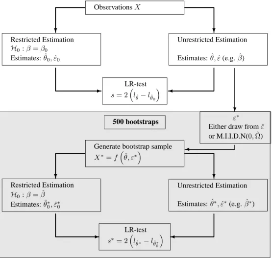
Defining Θ the entire parameter set of the VAR and assuming we are interested in the test H0 : β = β0 we thus implement the following bootstrap procedure, which is
graphically represented in figure 1
• Bootstrap test
1. Estimate VAR on dataX; for given cointegrating rank obtain unrestricted estimates
ˆ
θ, unrestricted residuals εb, restricted estimates θˆ0, restricted residuals εb0 and test
statisticsfor the hypothesisH0 :β =β0;
2. Construct pseudodata:X∗ =φ(ˆθ, ε∗), ε∗drawn at random with replacement fromεb orNID.
3. Estimate VAR on pseudodata X∗; obtain θˆ∗,εb∗, θˆ0∗,bε∗0 and test statistics∗ for the hypothesisH0∗:β = ˆβ;
Repeat (2)-(3) a large number of times
(4) Compute bootstrap p-value: p∗ =prop(s∗ > s).
The test statistic is the likelihood ratio test (which is the only one allowing a Bartlett correction).
3Note that there is a possible source of confusion here, as the terms ‘parametric’ and ‘non-parametric’
have been used in the bootstrap literature with different meanings. We define procedures based on re-sampling from estimated residuals as ‘non parametric’, and that involving drawings from a theoretical distribution as ‘parametric’.
ObservationsX ? ? -Restricted Estimation H0:β =β0 Estimates:θˆ0,εˆ0 Unrestricted Estimation Estimates:θ,ˆ εˆ(e.g.βˆ) LR-test s= 2³lθˆ−lθˆ0 ´ 500 bootstraps ε ∗
Either draw fromεˆ
or M.I.I.D.N(0,Ωˆ) Generate bootstrap sample
X∗=f³θ, εˆ ∗´ ? ? -? Restricted Estimation H0:β = ˆβ Estimates:θˆ∗0,εˆ∗0 Unrestricted Estimation Estimates:θˆ∗,εˆ∗(e.g.βˆ∗) LR-test s∗= 2³l ˆ θ∗−lθˆ∗ 0 ´
Calculate bootstrap p-value
p∗=prop(s∗> s)
Figure 1: Bootstrap procedure for tests on the cointegration parameters
If we have a simple hypothesis on only part of the cointegration space,β1 = β01, we
take the following null hypothesis in step 3:
β1 = ˆβ0( ˆβ0βˆ)−1βˆ0β10 (6)
which is easily seen to converge toβ10ifH0 is true.
As mentioned in the introduction, Davidson and MacKinnon (2000) recently put forth a computationally cheap double bootstrap procedure which may deliver results superior to the standard bootstrap just outlined4. The idea behind the double bootstrap, proposed
by Beran (1988) is that of correcting the possible bias in the bootstrap procedure imple-mented by a second application of the bootstrap. For instance, in the case of a test the aim of the second-level application of the bootstrap would be to estimate, and thus correct for, the bias(pi −i), where pi is the p-value of the i-level bootstrap test. Although the
principle is certainly attractive, it is also very expensive, as it involves the construction of a bootstrap pseudo-population for each bootstrap redraw. It is thus practically impossible to evaluate by means of Monte Carlo experiments with the currently available computing power. On the contrary, in Davidson and MacKinnon’s method there is only one second level bootstrap redraw for each first level one, so that the computing time is of the same order of magnitude of the standard bootstrap. Monte Carlo experiments are thus feasible. Going into the details of the method is clearly beyond the scope of this paper. However, the basic intuition is very simple: if the bootstrap estimate p∗ = prop(s∗ > s)of true
p-value of the test is distorted, we may get a better estimate by replacing s with somees chosen so to counterbalance the distortion. Now,s is by definition thep∗ −th quantile of the distribution of thes∗; hence, an obvious candidate foresis the same quantile of the distribution of a second-level bootstrap distribution. Ifp∗ is distorted downwards, such a quantile will tend to be larger than the true quantiles, and viceversa, thus delivering the desired effect.
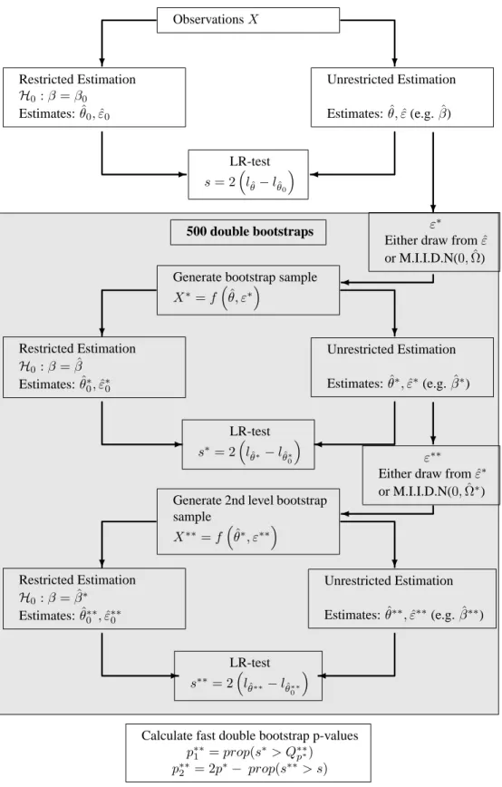
The general structure of the fast double bootstrap test we shall implement is the fol-lowing: (see figure 2 for a graphical representation)
• Fast Double Bootstrap test
1. Estimate VAR on dataX; for given cointegrating rank obtain estimatesθ,ˆ bε,θˆ0,εb0
and test statisticsfor the hypothesisH0 :β =β0;
2. Construct pseudodata:X∗ =φ(ˆθ, ε∗), ε∗drawn at random with replacement fromεb orNID;
3. Estimate VAR on pseudodata X∗; obtain θˆ∗,εb∗, θˆ0∗,bε∗0 and test statistics∗ for the hypothesisH0∗:β = ˆβ;
4Although Davidson and MacKinnon’s analytical results are valid only for one-sided tests with
totic N(0,1) distributions, some simulation evidence suggests that the properties may extend to the asymp-toticχ2of interest here.
ObservationsX ? ? -Restricted Estimation H0:β =β0 Estimates:θˆ0,εˆ0 Unrestricted Estimation Estimates:θ,ˆ εˆ(e.g.βˆ) LR-test s= 2³lθˆ−lθˆ0 ´ 500 double bootstraps ε ∗
Either draw fromεˆ
or M.I.I.D.N(0,Ωˆ) Generate bootstrap sample
X∗=f³θ, εˆ ∗´ ? ? -? Restricted Estimation H0:β = ˆβ Estimates:θˆ∗ 0,εˆ∗0 Unrestricted Estimation Estimates:θˆ∗,εˆ∗(e.g.βˆ∗) LR-test s∗= 2³l ˆ θ∗−lθˆ∗ 0 ´ ε∗∗
Either draw fromεˆ∗ or M.I.I.D.N(0,Ωˆ∗)
Generate 2nd level bootstrap sample X∗∗=f³θˆ∗, ε∗∗´ ? ? -? Restricted Estimation H0:β = ˆβ∗ Estimates:θˆ∗∗ 0 ,εˆ∗∗0 Unrestricted Estimation Estimates:θˆ∗∗,εˆ∗∗(e.g.βˆ∗∗) LR-test s∗∗= 2³l ˆ θ∗∗−lθˆ∗∗ 0 ´
Calculate fast double bootstrap p-values
p∗∗
1 =prop(s∗> Q∗∗p∗)
p∗∗
2 = 2p∗− prop(s∗∗> s)
Figure 2: Fast Double Bootstrap procedure for tests on the cointegration parameters 10
4. Construct second-level pseudodataX∗∗ =φ(ˆθ∗, ε∗∗), ε∗∗drawn at random with re-placement fromεb∗ orNID;
5. Estimate VAR on second-level pseudodata X∗∗; obtain θˆ∗∗,εb∗∗, θˆ∗∗0 ,bε∗∗0 and test statistic s∗∗for the hypothesisH0∗∗:β = ˆβ∗;
Repeat (2)-(5) a large number of times
(6) Compute bootstrap p-value: p∗ =prop(s∗ > s).
(7) Compute fast double bootstrapp-value type 1:p∗∗1 =prop(s∗ > Q∗∗p∗),whereQ∗∗p∗is
thep∗quantile of thes∗∗’s.
A (costless) further step is advisable:
(8) Compute fast double bootstrapp-value type 2: p∗∗2 = 2p∗ − prop(s∗∗> s).
Again, the intuition here is that if for instancep∗ > p,we can expectprop(s∗∗> s)>
p∗,so thatp∗∗
2 will be closer topthanp∗. However,p∗∗2 may not be greater than 2p∗ and
it may be negative, two undesirable features that suggest limiting its use to a reliability check: if the difference between the twop-values is sizebale neither of them should be trusted.
3
Design of the Monte Carlo Experiment
On the basis of the simulation results reported by Gredenhoff and Jacobson (2001) and Fachin (2000), the key characteristics of the DGP to be controlled in the experiments are the dimension of the system, i.e. number of variables and lags, and its long-run structure, i.e. number of the cointegrating relationships and the speed at which the system adjusts to them. Estimation of systems of higher dimension (both in terms of number of variables and lags) demand more from the data, and thus it is (ex-post) not surprising to see that both the asymptotic test and the bootstrap test proposed by Gredenhoff and Jacobson (2001) perform better in smaller systems. A crucial remark here is that the simple bivariate DGPs employed in virtually all simulation studies do suffer from loss of generality, a fact not suspected so far. The experimental design adopted here will thus generalize to a multivariate system the classical DGP used by a number of studies starting with Engle and Granger (1987), which allows an easy control of the speed of adjustment. We shall consider systems including p = 5 random variables and withr = 1 or 2 cointegrating relationships. Letxt= [x1t. . . x5t]0be the column vector of the realizations of the random
variables of interest at timet = 1, . . . , T , ut = [u1t. . . u5t]0 the errors, ²t = [ε1t. . . ε5t]0
the noise, whose stochastic structure will be discussed in detail below, andta time trend. Our DGP is then given by
β0 1 .. . β0 5 · xt t ¸ =ut (7) Φut=²t (8) with Φ =diag(φ),φ=£ φ1(L) φ2(L) φ3(L) φ4(L) φ5(L) ¤ .
Although the Bartlett corrections do depend on the parameters of the system, in order to keep the size of the experiment within manageable dimensions in the size simulations the cointegrating coefficients will be kept fixed across trials to either zero or1, with the vectors resembling quite closely those used by Haug (1996), while in the power simu-lations we shall consider a few values in the range[0.5,1.5]. Given that we are using a full-information method we do not need to worry about endogeneity; we shall thus con-sider a very simple structure, with one stochastic trend (Xp) transmitted to the first r
variables of the system, while the remainingp−r−1follow independent random walks. The details in the two cases are as follows:
(a) r = 1
β1 =
£
1 0 0 0 β15 0.01
¤
is the cointegration vector. All the other relations are non-stationary:
β2 = £ 0 1 0 0 0 0 ¤;β3 = £ 0 0 1 0 0 0 ¤; β4 = £ 0 0 0 1 0 0 ¤;β5 = £ 0 0 0 0 1 0 ¤; φ1(L) = (1, ϕ1L, . . . , ϕkLk); φ2(L) = φ3(L) =φ4(L) =φ5(L) = (1,−L). (b) r = 2 β2 = £
0 1 0 0 1 0.01 ¤becomes a cointegration vector. All the otherβ0sare as in case(a).
φ1(L) = φ2(L) = (1, ϕ1L, . . . , ϕkLk);
φ3(L) = φ4(L) =φ5(L) = (1,−L).
Some simple considerations will allow great simplification of the design as far as the
ε0s are concerned. First of all, in previous work on the related topic of stationary VARs
Fachin and Bravetti (1996) found that the shape of the distribution of the shocks does not appear to have a significant impact on the performances of asymptotic procedures. Further, the expectation that with a full-information method, their covariance structure should not matter either has been confirmed in the case of a simple bivariate DGP by Fachin (2000). We shall thus assumeε= [ε1. . . εp]∼MIIDN(0, I).
Finally, the number of both Monte Carlo replications and bootstrap redrawings has been fixed to 500: on the basis of previous work and some pilot experiments we concluded that the gain in precision deliver by higher numbers of either was not worth the higher computing costs and longer calendar time required. At 0.05 the Monte Carlo standard error will thus be about 0.010.
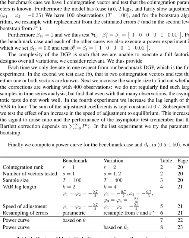
In table 1 we give an overview of the parameter values in the various experiments. In the benchmark case we have 1 cointegration vector and test that the cointegration param-eters is known. Furthermore the model has (case (a)), 2 lags, and fairly slow adjustment
(ϕ1 =ϕ2 =−0.35) We have 100 observations (T = 100), and for the bootstrap
algo-rithm, we resample with replacement from the estimated errorsεˆ(and in the second level bootstrap fromεˆ∗ ).
Furthermoreβ15 = 1and we thus testH0 :β10 =β1 =
£
1 0 0 0 1 0.01 ¤. For the benchmark case and each of the other cases we also execute a power experiment in which we setβ15= 0.5and testβ10 =β1 =
£
1 0 0 0 1 0.01 ¤.
The complexity of the DGP is such that we are unable to execute a full factorial designo over all variations, we consider relevant. We thus provide
Each time we only deviate in one respect from our benchmark DGP, which is the first experiment. In the second we test case (b), that is two cointegration vectors and test that either one or both vectors are known. Next we increase the sample size to find out whether the corrections are working with 400 observations: we do not regularly find such large samples in time series analysis, but find that even with that many observations, the asymp-totic tests do not work well. In the fourth experiment we increase the lag length of the VAR to four. The sum of the adjustment coefficients is kept constant at0.7. Subsequently we test the effect of an increase in the speed of adjustment to equilibrium. This increases the signal to noise ratio and the performance of the asymptotic test (remember that the Bartlett correction depends on P∞i=0Pi). In the last experiment we try the parametric bootstrap.
Finally we compute a power curve for the benchmark case andβ15in(0.5,1.50), with
Benchmark Variation Table Page Cointegration rank r= 1 r= 2 2 20 Number of vectors tested s= 1 s= 1,2 2 20 Sample size T = 100 T = 400 3 20
VAR lag length k = 2 k = 4 4 21
ϕ1 =ϕ2 =−02.7 ϕ1 =−02.7, ϕ2 =−03.7,
ϕ3 =ϕ4 =−016.7
Speed of adjustment ϕ1 =ϕ2 =−02.7 ϕ1 =ϕ2 =−02.4 5 21
Resampling of errors parametric resample frombεandbε∗ 6 21
Power curve based onθˆ 7 22
Power curve based onθˆ0 8 23
β0
15 = 1as usual, both for the bootstrap and Bartlett correction we propose, that is those
based on the estimates under the alternative and one based on estimates under the null.
4
Results
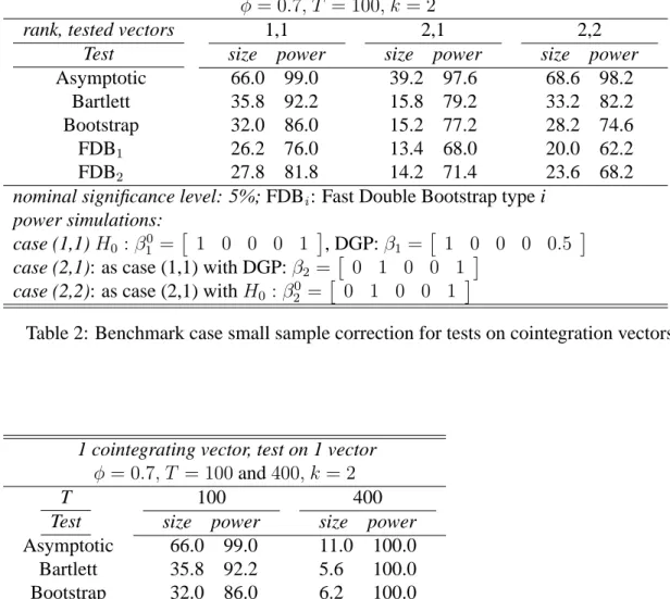
Although the results of the simulations amount to a considerable mass, their essence is quite simple, and summarised in Table 2; in the following tables a few details are high-lighted, with baseline results repeated in different tables in order to facilitate comparisons. In all the cases reported and discussed in this section the nominal significance level of the tests is always 5%, with results for different values available on request.
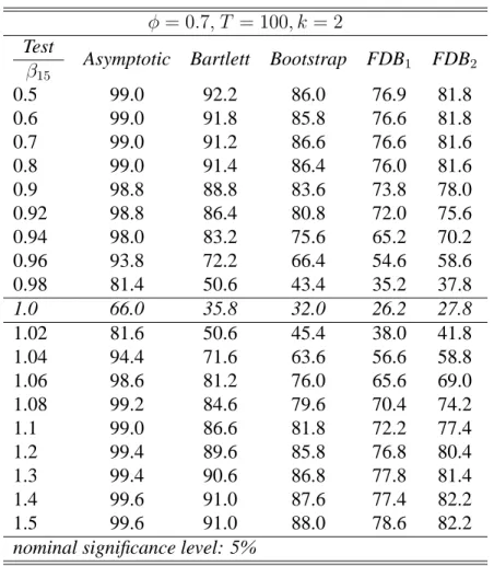
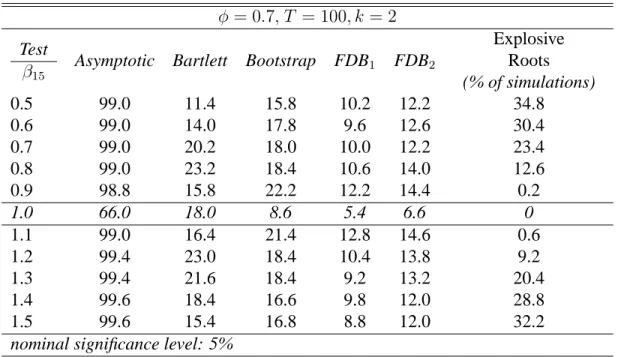
First of all, in the sample sizes we typically encounter in applied econometric work (100 observations) the asymptotic tests deliver disastrous performance as far as type I er-rors are concerned: at times they exceed 50% at the nominal 5% level. All the alternative procedures (Bartlett correction, simple and fast double bootstrap) are able to reduce sub-stantially the size distortion in all our experiments, but are unable to eliminate it: in the case of rank=1 the minimum rejection rate, delivered by the fast double bootstrap type 1, is 26%, while in the case of rank=2 and test on one vector the rejection rate of all bootstrap procedures and the Bartlett corrected test is 15%. The two types of fast double bootstrapp-values are always very close, confirming that the procedure is reliable in our context. The power loss from using the procedures with lower size distortion is accept-able, with the rejection rates always over 70%. This finding will be confirmed by the power curve reported in table 7. To understand the point of basing both the bootstrap and Bartlett correction on the unrestricted estimates, a glance at the power curves in table 8 suffices: whereas the size performance is indeed slightly better than in table 7, the level of type II errors is unacceptably high, such that the power curves are almost flat. In the last row we report the number of cases where the highest estimated root is explosive: when the discrepancy between DGP and model becomes large, this percentage rises rapidly and corroborates theorem 1 of this paper5.
Another key point from Table 2, is that the size performance of all test procedures of
H0 : β1 = β10in a model with 2 vectors is markedly better than the hypothesisH0 :β =
β0 in a model with one cointegrating vector.
ForT = 400all corrected tests achieve correct size and 100% power while the Type I error of the asymptotic test is still higher than the nominal size (cf. Table 3).
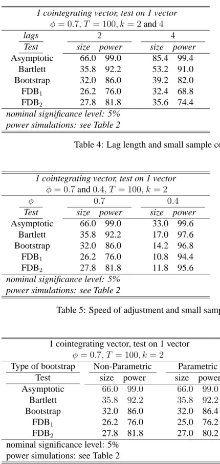
Increasing the length of the VAR also has large adverse effects on the test (cf. Table 4): thus, contrary to somehow common wisdom and in accord with Abadir et al. (1999), parsimony in the estimation of the VAR seems to be a rather important virtue.
5tr(P∞
i=0Pi)does not converge ifPcontains an explosive root. However computationally we use the standard formula(P∞i=0λi) = 1−1λ to calculate the Bartlett correction both in the convergent case (when it is valid) and the non-convergent case.
There is nothing, which prevents the Bartlett correction factor from being smaller than -1: this is a known problem in the literature. We assign a p-value of 1 to these cases. In all the published and unpublished simulations we did, this only happened in those of table 8.
How sensitive are the performances of the tests to the speed of adjustment to equi-librium? Unsurprisingly, the answer is, a lot. Cuttingφ (the sum of the coefficients of the autoregressive polynomial describing the dynamics of the errors in the cointegrating relationships) from 0.7 to 0.4 causes generally a more than proportional fall of the Type I error (for instance, that of the fast double bootstrap type 1 falls from 26% to 10%, see table 5).
Given the good results delivered by the bootstrapped tests, it is of some interest to check if using resampled or parametrically generated errors makes any difference. The results reported in Table 6 suggest that it does not, and thus the parametric bootstrap (easier to implement) may be adopted in practice. However, some caution is needed here, as in our experiments the same parametric hypothesis (normality) is used both in the generation of the Monte Carlo and bootstrap errors. Further research with different error processes for the Monte Carlo and bootstrap DGPs (for instance a leptocurtic error distribution in the DPG and resampling for a normal distribution) is needed.
Finally, a noteworthy finding is that the power curves of the all the variants of boot-strap tests are rather steep (table 7 and figure 3(b)). Although these results are specific to a single signal/noise ratio, they do suggest that the risk of unacceptable power losses from using some type of bootstrap test rather than the asymptotic or Bartlett corrected tests is likely to be remote.
5
Conclusions
We have compared different variants of bootstrap and Bartlett-corrected tests in a DGP which is relatively unfavourable, but reproduces some features of real life empirical appli-cations: a relatively large system (5 variables and 2 or 4 lags), and rather slow adjustment to long-run equilibrium. With such a complex DGP the caveats common to all simulation studies are even more important than usual. Our design depends on over 120 parameters, the vast majority of which had to be kept fixed across all experiments, and thus we must be extremely cautious in reaching any conclusion.
Further, the type of tests examined assumes full knowledge of the tested cointegrating vectors, a rare event in practice: however, they are the only tests for which the Bartlett correction is available. Indeed, the Bartlett correction has not been derived yet for many cases of strong empirical interest (e.g., hypotheses of the kindβi =Hiϕi and in general
models with impulse dummies) and hence the bootstrap may in fact be the only alter-native to the asymptoticp-values. With all these caveats, our recommendations are the following:
(i) Asymptotic tests should be used in no circumstance;
(ii) Bartlett-corrected tests may be used provided considerable caution is exercised, as
their Type I error is often much larger than the nominal size;
(iii) Bootstrap tests, with a somehow lower size distortion than the Bartlett corrected
boot-strap of Davidson and MacKinnon (2000) delivers the best performance, and thus it appears to be a powerful tool for applied work, especially in the many cases when the Bartlett correction is not available.
We stress that both the Bartlett correction and the bootstrap should always be based on the unrestricted estimate ofβ.
Among the many points that remain open, two are especially important: (a) the devel-opment of equivalent hypothesis, like (6) forH0 : β1 = β10 for more general restrictions
onβ, likeβi =Hiϕi with an accurate Monte Carlo study of their properties and (b)
theo-retical results on the asymptotics of the (fast double) bootstrap in cointegrated systems.
References
Abadir, K., K. Hadri, and E. Tzavalis (1999). The influence of VAR dimensions on estimator biases. Econometrica 67, 163–181.
Barndorff-Nielsen, O. and P. Hall (1988). On the level-error after Bartlett adjustment of the likelihood ratio statistic. Biometrika 75, 374–378.
Bartlett, M. (1937). Properties of sufficiency and statistical tests. Proceedings of the
Royal Society of London Series A 160, 268–282.
Beran, K. (1988). Prepivoting test statistics: A bootstrap view of asymptotic refinements.
Journal of the American Statistical Association 83, 687–697.
Berkowitz, J. and L. Kilian (2000). Recent developments in bootstrapping time series.
Econometric Reviews 19, 1–48.
Bewley, R., D. Orden, M. Yang, and L. Fisher (1994). Comparison of Box-Tiao and Johansen canonical estimator of cointegration vectors in VEC(1) models. Journal of
Econometrics 64, 3–27.
Chan, N. and C. Wei (1988). Limiting distributions of least squares estimates of unstable autoregressive processes. Annals of Mathematical Statistics 16, 367–410.
Chang, Y., R. Sickles, and W. Song (2001). Bootstrapping unit root tests with covariates. Technical report, Rice University.
Cribari-Neto, F. and G. Cordeiro (1996). On Bartlett and Bartlett-type corrections.
Econo-metric Reviews 15, 339–367.
Davidson, J. (2001). Alternative bootstrap procedures for testing cointegration in frac-tionally integrated processes. Technical report, Cardiff University.
Davidson, R. and J. MacKinnon (2000). Improving the reliability of bootstrap tests. Tech-nical Report 995, Queen’s University Institute for Economic Research.
Efron, B. and R. Tibshirani (1993). An Introduction to the Bootstrap. London: Chapman & Hall.
Engle, R. and C. Granger (1987). Co-integration and error correction: Representation, estimation and testing. Econometrica 55, 251–276.
Fachin, S. (2000). Bootstrap and asymptotic tests of long-run relationships in cointegrated systems. Oxford Bulletin of Economics and Statistics 62, 577–585.
Fachin, S. and L. Bravetti (1996). Asymptotic normal and bootstrap inference in structural VAR analysis. Journal of Forecasting 15, 329–341.
Gonzalo, J. (1994). Five alternative methods of estimating long-run equilibrium relation-ships. Journal of Econometrics 64, 203–233.
Gredenhoff, M. and T. Jacobson (2001). Bootstrap testing linear restrictions on cointe-grating vectors. Journal of Business and Economic Statistics 19, 63–72.
Hall, P. (1992). The Bootstrap and Edgeworth Expansion. New York: Springer.
Hall, P. (1995). Methodology and theory for the bootstrap. In R. Engle and D. McFadden (Eds.), Handbook of Econometrics, Vol. IV, Amsterdam. North-Holland.
Haug, A. (1996). Tests for cointegration - a Monte Carlo comparison. Journal of
Econo-metrics 71, 89–115.
Horowitz, J. (2002). The bootstrap. In J. Heckman and E. Leamer (Eds.), Handbook of
Econometrics, Vol. V, Amsterdam. North-Holland.
Inoue, A. and L. Kilian (2002). Bootstrapping autoregressive processes with possible unit roots. Econometrica 70, 377–391.
Jensen, J. and A. Wood (1997). On the non-existence of a Bartlett correction for unit root tests. Statistics and Probability Letters 35, 181–187.
Johansen, S. (1991). Estimation and hypothesis testing of cointegration vectors in Gaus-sian vector autoregressive processes. Econometrica 59, 1551–1580.
Johansen, S. (1995). Likelihood-Based Inference in Cointegrated Vector Autoregressive
Models. Oxford: Oxford University Press.
Johansen, S. (2000). A Bartlett correction factor for tests on the cointegrating relations.
Econometric Theory 16, 740–778.
Lawley, D. (1956). A general method for approximating the distribution for the likelihood ratio criteria. Biometrika 43, 293–303.
Li, H. and G. Maddala (1996). Bootstrapping time series models. Econometric
Li, H. and G. Maddala (1997). Bootstrapping cointegrating regressions. Journal of
Econo-metrics 80, 297–318.
Nielsen, B. (1997). Bartlett correction of the unit root test in autoregressive models.
Biometrika 84, 500–504.
Paparoditis, E. and D. Polititis (2001). Unit-roots testing via the continuos-path block bootstrap. Technical Report 2001-06, University of California at San Diego, Depart-ment of Economics.
Phillips, P. (2001). Bootstrapping spurious regression. Technical report.
Appendix: Figures and tables
0.5
1
1.5
0
20
40
60
80
100
Asymptotic
Bartlett
Bootstrap
FDBS 1
FDBS 2
(a) power curves based on restricted estimatesθˆ0
0.5
1
1.5
0
20
40
60
80
100
Asymptotic
Bartlett
Bootstrap
FDBS 1
FDBS 2
(b) power curves based on unrestricted estimatesθˆ
1 to 2 cointegration vectors, test on 1 to 2 vectors
φ= 0.7, T = 100, k = 2
rank, tested vectors Test 1,1 size power 2,1 size power 2,2 size power Asymptotic Bartlett Bootstrap FDB1 FDB2 66.0 99.0 35.8 92.2 32.0 86.0 26.2 76.0 27.8 81.8 39.2 97.6 15.8 79.2 15.2 77.2 13.4 68.0 14.2 71.4 68.6 98.2 33.2 82.2 28.2 74.6 20.0 62.2 23.6 68.2
nominal significance level: 5%; FDBi: Fast Double Bootstrap type i
power simulations: case (1,1)H0 :β10 = £ 1 0 0 0 1 ¤, DGP:β1 = £ 1 0 0 0 0.5 ¤
case (2,1): as case (1,1) with DGP:β2 =
£
0 1 0 0 1 ¤
case (2,2): as case (2,1) withH0 :β20 =
£
0 1 0 0 1 ¤
Table 2: Benchmark case small sample correction for tests on cointegration vectors
1 cointegrating vector, test on 1 vector
φ= 0.7, T = 100and400, k = 2 T Test 100 size power 400 size power Asymptotic Bartlett Bootstrap FDB1 FDB2 66.0 99.0 35.8 92.2 32.0 86.0 26.2 76.0 27.8 81.8 11.0 100.0 5.6 100.0 6.2 100.0 5.6 100.0 5.8 100.0
nominal significance level: 5% power simulations: see Table 2
Table 3: Sample size and small sample corrections
1 cointegrating vector, test on 1 vector φ = 0.7, T = 100, k= 2and4 lags Test 2 size power 4 size power Asymptotic Bartlett Bootstrap FDB1 FDB2 66.0 99.0 35.8 92.2 32.0 86.0 26.2 76.0 27.8 81.8 85.4 99.4 53.2 91.0 39.2 82.0 32.4 68.8 35.6 74.4
nominal significance level: 5% power simulations: see Table 2
Table 4: Lag length and small sample corrections
1 cointegrating vector, test on 1 vector
φ= 0.7and0.4, T = 100, k = 2 φ Test 0.7 size power 0.4 size power Asymptotic Bartlett Bootstrap FDB1 FDB2 66.0 99.0 35.8 92.2 32.0 86.0 26.2 76.0 27.8 81.8 33.0 99.6 17.0 97.6 14.2 96.8 10.8 94.4 11.8 95.6
nominal significance level: 5% power simulations: see Table 2
Table 5: Speed of adjustment and small sample corrections
1 cointegrating vector, test on 1 vector
φ = 0.7, T = 100, k= 2 Type of bootstrap Test Non-Parametric size power Parametric size power Asymptotic Bartlett Bootstrap FDB1 FDB2 66.0 99.0 35.8 92.2 32.0 86.0 26.2 76.0 27.8 81.8 66.0 99.0 35.8 92.2 32.0 86.4 25.0 76.2 27.0 80.2 nominal significance level: 5%
power simulations: see Table 2
φ= 0.7, T = 100, k = 2
Test
β15 Asymptotic Bartlett Bootstrap FDB1 FDB2
0.5 99.0 92.2 86.0 76.9 81.8 0.6 99.0 91.8 85.8 76.6 81.8 0.7 99.0 91.2 86.6 76.6 81.6 0.8 99.0 91.4 86.4 76.0 81.6 0.9 98.8 88.8 83.6 73.8 78.0 0.92 98.8 86.4 80.8 72.0 75.6 0.94 98.0 83.2 75.6 65.2 70.2 0.96 93.8 72.2 66.4 54.6 58.6 0.98 81.4 50.6 43.4 35.2 37.8 1.0 66.0 35.8 32.0 26.2 27.8 1.02 81.6 50.6 45.4 38.0 41.8 1.04 94.4 71.6 63.6 56.6 58.8 1.06 98.6 81.2 76.0 65.6 69.0 1.08 99.2 84.6 79.6 70.4 74.2 1.1 99.0 86.6 81.8 72.2 77.4 1.2 99.4 89.6 85.8 76.8 80.4 1.3 99.4 90.6 86.8 77.8 81.4 1.4 99.6 91.0 87.6 77.4 82.2 1.5 99.6 91.0 88.0 78.6 82.2
nominal significance level: 5%
Table 7: Power curve based on unrestricted estimates
φ = 0.7, T = 100, k= 2
Test
β15 Asymptotic Bartlett Bootstrap FDB1 FDB2
Explosive Roots (% of simulations) 0.5 99.0 11.4 15.8 10.2 12.2 34.8 0.6 99.0 14.0 17.8 9.6 12.6 30.4 0.7 99.0 20.2 18.0 10.0 12.2 23.4 0.8 99.0 23.2 18.4 10.6 14.0 12.6 0.9 98.8 15.8 22.2 12.2 14.4 0.2 1.0 66.0 18.0 8.6 5.4 6.6 0 1.1 99.0 16.4 21.4 12.8 14.6 0.6 1.2 99.4 23.0 18.4 10.4 13.8 9.2 1.3 99.4 21.6 18.4 9.2 13.2 20.4 1.4 99.6 18.4 16.6 9.8 12.0 28.8 1.5 99.6 15.4 16.8 8.8 12.0 32.2
nominal significance level: 5%