The Transmuted Inverse Exponential Distribution

doi: 10.14419/ijasp.v3i1.3684 Research Paper

The Transmuted Inverse Exponential Distribution

Oguntunde P. E 1*; Adejumo A. O 2

1

Department of Mathematics, Covenant University, Ota, Ogun State, Nigeria

2

Department of Statistics, University of Ilorin, Kwara State, Nigeria *Corresponding author E-mail:peluemman@yahoo.com

Copyright © 2014 Oguntunde P. E., Adejumo A. O. This is an open access article distributed under the Creative Commons Attribution License, which permits unrestricted use, distribution, and reproduction in any medium, provided the original work is properly cited.

Abstract

This article introduces a two-parameter probability model which represents another generalization of the Inverse Exponential distribution by using the quadratic rank transmuted map. The proposed model is named Transmuted Inverse Exponential (TIE) distribution and its statistical properties are systematically studied. We provide explicit expressions for its moments, moment generating function, quantile function, reliability function and hazard function. We estimate the parameters of the TIE distribution using the method of maximum likelihood estimation (MLE). The hazard function of the model has an inverted bathtub shape and we propose the usefulness of the TIE distribution in modeling breast cancer and bladder cancer data sets.

Keywords: Generalization; Inverse Exponential; Moments; Quadratic Rank Transmuted Map; Quantile Function; Transmuted Inverse Exponential.

1.

Introduction

The one parameter Exponential distribution describes the time between events in a Poisson process. Its discrete analogue is the Geometric distribution. Apart from its usage in Poisson processes, it has been used extensively in the literature for life testing. The Exponential distribution is memoryless and has a constant failure rate; this latter property makes the distribution unsuitable for real life problems with bathtub failure rates (See Singh et al [17] for details) and inverted bathtub failure rates, hence the need to generalize the Exponential distribution in order to increase its flexibility and capability to model some other real life problems. For details about the Exponential distribution, we refer readers to [12-15].

The one parameter Inverse Exponential distribution otherwise known as the Inverted Exponential distribution was introduced by Keller and Kamath [7]. It has an inverted bathtub failure rate and it is an important competitive model for the Exponential distribution. It has been identified and discussed by Lin et al [9] as a lifetime model. If X is a non-negative Exponential random variable, then the distribution of a random variable Y 1

X

 follows an Inverse Exponential distribution. Hence, if X denotes a random variable, the cumulative density function (cdf) and the probability density function (pdf) of the Inverse Exponential distribution with a scale parameter  are respectively given by; ( ) exp F x x   _ _   (1) ( ) exp 2 f x x x    _ _   (2)

Wherex 0, the scale parameter  0

A generalization of the Inverse Exponential distribution called the Kumaraswamy-Inverse Exponential distribution has been defined and studied by Oguntunde et al [12].

Shaw and Buckley [16] studied the quadratic rank transmutation map (QRTM) and in recent times, several authors have used the understanding to generalize several known theoretical models. For instance, Aryal and Tsokos [2] generalized

the Weibull distribution using the QRTM and named the resulting distribution the Transmuted Weibull distribution. In the same manner, the Transmuted Rayleigh distribution by Merovci [10], Transmuted Exponentiated Modified Weibull Distribution by Ashour and Eltehiwy [3], Transmuted Modified Weibull distribution by Khan et al [8], Transmuted Lomax distribution by Ashour and Eltehiwy [4], Transmuted Exponentiated Gamma distribution by Hussian [6], Transmuted Inverse Rayleigh distribution by Ahmad et al [1], Transmuted Pareto distribution by Merovci and Puka [11], Transmuted Inverse Weibull distribution by [5], [8] are noticeable examples in the literature.

This article seeks to develop another generalization of the Inverse Exponential distribution by using the QRTM proposed by Shaw and Buckley [16]. The statistical properties of the resulting model shall also be systematically studied. The rest of this article is organized as follows; Section 2 introduces the proposed Transmuted Inverse Exponential distribution including a study of some of its basic statistical properties, Section 3 gives the estimation of the model parameters using the method of maximum likelihood estimation (MLE), followed by a concluding remark.

2.

The Transmuted Inverse Exponential Distribution

Starting from an arbitrary parent cumulative density functionF x₁( ), a random variable X is said to have a transmuted distribution if its cdf is given by;

2

( ) (1 ) ( ) ( )

2 1 1

F x   F x F x (3) Differentiating Equation (3) with respect to

x

gives;

( ) ( ) 1 2 ( )

2 1 1

f x f x _   F x _ (4) Where| | 1, f₁( )x and f₂( )x are the associated pdf of F x₁( ) and F x₂( ) respectively.

It is good to note that if 0; Equation (3) and (4) reduces to the parent distribution.

Hence, a random variable X is said to have a Transmuted Inverse Exponential distribution with parameters



and



if the cumulative density function is given by;

( ) exp 1 exp F x x x     _ _ _ _   _ __         (5)

The corresponding pdf is given by;

( ) exp 1 2 exp 2 f x x x x   _{ }   _ __   _ __     (6) For

x



0,





0

and

|



| 1



. where



is the scale parameter



is the transmuted parameter

For notational purposes, we write; X : TIE( , ) 

By choosing various values for parameters  and, we provide a possible shape for the pdf of the TIE distribution as shown in Figure 1 below;

Fig. 1: Plot for the TIE pdf at Various Parameter Values Relationship with other distributions

Some well-known theoretical distributions can be derived from the proposed TIE distribution. For instance; 1) For 0, Equation (6) reduces to give the one-parameter Inverse Exponential distribution.

2) If a random variable Y is such that Y 1 X

 and  0 in Equation (6) then we have the Exponential distribution. The plot for the TIE cdf at various parameters values of  and  is shown below in Figure 2 as;

0 0.02 0.04 0.06 0.08 0.1 0.12 0.14 0.16 1 3 5 7 9 11 13 15 17 19 P D F X-values α=7, λ=1 α=8, λ=0.5 α=8, λ= - 0.5

Fig. 2: Plot for the TIE cdf at Various Parameter Values

2.1. Some Properties of the TIE distribution

This section provides some of the statistical properties of the TIE distribution.

2.1.1. Moments

The r-th moment of a random variable X, _r is given by; r

E X r

  _ _

Therefore, the r-th moment for the TIE distribution is given by;

exp 1 2 exp 2 0 r x dx r x x x      _ _    _ _  



1



exp 2 exp 2 2 2 0 0 r r x dx x dx r x x x x         _ _   _  _{ }_     

After some calculations,



1

 

1



2

r r

r r

    _   _ (7) We observe that Equation (7) only exists whenr1. The implication is that the first moment, second moment and other higher-order moments does not exist.

2.1.2. Moment generating function

The moment generating function (mgf) of a random variable X is given by;

 

 

tX M_X t E e

Following Khan et al [8], we derive the mgf of the TIE distribution as follows;

  

1



exp 2 exp 2 2 2 0 0 M_X t tx dx tx dx x x x x           _  _       _{ }   (8)

By Taylor’s series expansion, Equation (8) gives;

  



2 2 1 exp 2 exp 2 ! ! 2 0 0 0 0 k k t _k t _k M_X t x dx x dx k x k k k                                     

Hence, the mgf of the TIE distribution is given by;

  



   

 

2





1 1 1 ! ! 0 0 k k k t t M_X t k k k k k k                  (9)

2.1.3. The Quantile function and median

The Quantile of the Transmuted Inverse Exponential distribution is the real solution of the equation;

0 0.2 0.4 0.6 0.8 1 1 3 5 7 9 11 13 15 17 19 C D F X-values α=6, λ=1 α=7, λ=0.8 α=8, λ=0.5

   

1 2 log 2 1 1 4 X q q           





































(10)

Hence, the median of the distribution is derived by substituting q0.5 in Equation (10). That is,



 



2 log 0.5 ₂ 1 1 2 X                  _ _  _{ }  





1 2 log 0.5 ₂ 1 1 X                       (11) 2.1.4. Reliability Analysis

In this sub-section, we present the reliability function and the hazard function for the proposed TIE distribution.

The reliability function is otherwise known as the survival or survivor function. It is the probability that a system will survive beyond a specified time and it is obtained mathematically as the complement of the cumulative density function (cdf).

The survivor function is given by;

 









 

1

 

x

S x P X x f u du F x



  



 

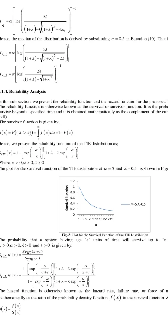
Hence, we present the reliability function of the TIE distribution as;

 

1 exp 1 exp TIE S x x x  _{ }   _ _ _ _   _ __         (12) Where x 0,0,0

The plot for the survival function of the TIE distribution at 5 and  0.5 is shown in Figure 3;

Fig. 3: Plot for the Survival Function of the TIE Distribution

The probability that a system having age ' 'x units of time will survive up to 'x t' units of time for

0, 0, 0

x    and t 0 is given by;

( ) ( | ) ( ) S_TIE x t S_TIE t x S_TIE x   1 exp 1 exp ( | ) 1 exp 1 exp x t x t S_TIE t x x x      _{ }                            _{ } _{ }                  _{ } _{ }     (13)

The hazard function is otherwise known as the hazard rate, failure rate, or force of mortality. It is obtained mathematically as the ratio of the probability density function

f x

 

to the survival function

S x

 

. It is given by;

 

f x

 

_{ }

h x x S  0 0.2 0.4 0.6 0.8 1 1.2 1 3 5 7 9 11 13 15 17 19 Sur vi val F unct ion x ∝=5,λ=0.5

 

 

_{ }

1 f x h x F x  

We thus present the hazard rate for the proposed TIE distribution as;

 

2exp 1 2 exp 1 exp 1 exp x x x h_TIE x x x   _{ }                                           _{ } _{ }     (14)

The plot for the hazard rate at various values of parameters  and  is shown in Figure 4;

Fig. 4: Plot for the Hazard Function of the TIE Distribution

We can infer from Figure 4 that the shape of the hazard rate is unimodal; it increases at the initial stage and later decreases. We can also say that the hazard rate shows an inverted bathtub shape.

3.

Estimation of Parameters and Inference

We estimate the parameters of the TIE distribution using the method of maximum likelihood estimation (MLE) as follows;

Let X₁,X₂,...,_{X n} be a random sample of ‘n’ independently and identically distributed random variables each having a TIE distribution defined in Equation (6), the likelihood function L is given by;

| , exp 1 2 exp 2 1 n L X x x i x                              _{ }_{  }_     : Let l logL X_ | , _   :

 

log 2 log log log 1 2 exp

1 1 1 n n n l n _{x i} x x i i _i i _i                       _  _        _  _     

Differentiating with respect to  and  respectively gives; 1 exp 1 2 1 1 1 2 exp x x n n dl n _{i i} d i x_i i x i         _                _{ }          _{  }      _{ }   _{ }     1 2 exp 1 1 2 exp x n dl i d i x i   _                          

Solving the nonlinear system of equations of dl 0

d  and 0 dl

d  gives the maximum likelihood estimates of  and  respectively.

Following Aryal and Tsokos [2], we obtain the 2 x 2 observed information matrix through;

0 0.05 0.1 0.15 0.2 1 3 5 7 9 11 13 15 17 19 H az ard Funct ion X-values α=7, λ=1 α=8, λ=0.8 α=8, λ=0.5

11 12 21 22 , V V N V V                               _{ }     _  _      : Where; 2 2 2 1 2 2 2 l l V E l l                      _{ }         (15)

The solution of the inverse matrix of the observed information matrix in Equation (15) gives the asymptotic variance and co-variance of the maximum likelihood estimators



 and





. The approximate 100 1









% asymptotic confidence intervals (C.I) for  and  are given by;

11 2 Z_ V   ; 22 2 Z_ V  

It is good to note that

2

Z_ is the  th percentiles of the standard normal distribution.

4.

Conclusion

We defined a two-parameter Transmuted Inverse Exponential distribution as a generalization of the one-parameter Inverse Exponential distribution. The model is positively skewed and its shape is unimodal, it also has an inverted bathtub failure rate. An explicit expression was provided for the r-th moment and the moment generating function. The moment for the distribution only exists forr1. The behavior of the hazard function indicates that the model is a competitive model for other probability models having inverted bathtub failure rates like the one parameter Inverse Exponential distribution and can serve as an alternative. Further research would involve assessing the flexibility of this model to that of the Kumaraswamy and Beta-counterpart distributions using real data sets. This new model can be used for modeling cases where the risk is low at the initial stage, increases with time and later decreases; for instance, cases of breast cancer and bladder cancer (among others).

Acknowledgements

We like to appreciate the efforts of the anonymous referees for their timely comments towards improving the quality of this article.

References

[1] Ahmad A., Ahmad S. P., and Ahmed A. “Transmuted Inverse Rayleigh Distribution: A Generalization of the Inverse Rayleigh Distribution”,

Mathematical Theory and Modeling, Vol. 4, No. 7, 2014.

[2] Aryal G. R., Tsokos C. P. “Transmuted Weibull Distribution: A Generalization of the Weibull Probability Distribution”, European Journal of Pure and Applied Mathematics, Vol. 4, No. 2, 2011, 89-102.

[3] Ashour S. K., and Eltehiwy M. A. “Transmuted Exponentiated Modified Weibull Distribution”, International journal of Basic and Applied Sciences, 2013a, Vol 2(3) 258-269.

[4] Ashour S. K., and Eltehiwy M. A. “Transmuted Lomax Distribution”, American Journal of Applied Mathematics and Statistics, 2013b, Vol. 1, No. 6, 121-127. http://dx.doi.org/10.12691/ajams-1-6-3.

[5] Elbatal I. “Transmuted Modified Inverse Weibull Distribution: A Generalization of the Modified Inverse Weibull Probability Distribution”

International Journal of Mathematical Archive, 4 (8), 2013, 117-129.

[6] Hussian M. A. “Transmuted Exponentiated Gamma Distribution: A Generalization of the Exponentiated Gamma Probability Distribution”,

Applied Mathematical Sciences, Vol. 8, 2014, No. 27, 1297-1310.

[7] Keller, A. Z and Kamath, A. R (1982). “Reliability analysis of CNC Machine Tools”. Reliability Engineering. Vol. 3, pp. 449-473. http://dx.doi.org/10.1016/0143-8174(82)90036-1.

[8] Khan M. S., King R. and Hudson I. L. “Characteristics of the transmuted inverse weibull distribution”, ANZIAM J. 55 (EMAC2013) pp. C197-C217, 2014.

[9] Lin, C. T, Duran, B. S and Lewis, T. O. “Inverted Gamma as life distribution”. Microelectron Reliability, Vol. 29 (4), (1989) 619-626. http://dx.doi.org/10.1016/0026-2714(89)90352-1.

[10] Merovci, F., “Transmuted Rayleigh Distribution”, Austrian Journal of Statistics, Vol. 42 (1), 21-31, 2013 [11] Merovci F., Puka L., “Transmuted Pareto Distribution”, ProbStat Forum, Volume 07, January 2014, Pages 1-11.

[12] Oguntunde P. E., Babatunde O. S., and Ogunmola A. O., “Theoretical Analysis of the Kumaraswamy-Inverse Exponential Distribution”

International Journal of Statistics and Applications, Vol. 4, No. 2, (2014), 113-116.

[13] Oguntunde P. E., Odetunmibi O. A., & Adejumo A. O., “A Study of Probability Models in Monitoring Environmental Pollution in Nigeria,”

Journal of Probability and Statistics, vol. 2014, Article ID 864965, 6 pages, 2014. doi:10.1155/2014/864965. http://dx.doi.org/10.1155/2014/864965.

[14] Oguntunde, P. E, Odetunmibi, O. A., Adejumo A. O. “On the Sum of exponentially distributed random variables: A convolution approach”.

European Journal of Statistics and Probability, 2(1), 1-8, 2014. http://dx.doi.org/10.1155/2014/864965.

[15] Oguntunde P. E, Odetunmibi O. A, Edeki S. O, Adejumo A. O., “On the modified ratio of exponential distributions” Bothalia Journal, vol 44, no 4, pp. 166-174, 2014.

[16] Shaw W and Buckley, I. (2007).The alchemy of probability distributions: beyond Gram- Charlier expansions and a skew- kurtotic- normal distribution from a rank transmutation map. Research Report, 2007.

[17] Singh S. K., Singh U., Kumar M. “Estimation of Parameters of Generalized Inverted Exponential Distribution for Progressive Type-II Censored Sample with Binomial Removals”. Journal of Probability and Statistics. Volume 2013, Article ID 183652. http://dx.doi.org/10.1155/2013/183652.