Robust Standard Errors in Transformed Likelihood
Estimation of Dynamic Panel Data Models
Kazuhiko Hayakawa and M. Hashem Pesaran
May 2012
Robust Standard Errors in Transformed Likelihood
Estimation of Dynamic Panel Data Models
∗Kazuhiko Hayakawa Hiroshima University
M. Hashem Pesaran
University of Cambridge and USC
April 27, 2012
Abstract
This paper extends the transformed maximum likelihood approach for estimation of dynamic panel data models by Hsiao, Pesaran, and Tahmiscioglu (2002) to the case where the errors are cross-sectionally heteroskedastic. This extension is not trivial due to the incidental parameters problem that arises, and its implications for estimation and inference. We approach the problem by working with a mis-specified homoskedastic model. It is shown that the transformed maximum likelihood estimator continues to be consistent even in the presence of cross-sectional heteroskedasticity. We also obtain standard errors that are robust to cross-sectional heteroskedasticity of unknown form. By means of Monte Carlo simulation, we investigate the finite sample behavior of the transformed maximum likelihood estimator and compare it with various GMM estimators proposed in the liter-ature. Simulation results reveal that, in terms of median absolute errors and accuracy of inference, the transformed likelihood estimator outperforms the GMM estimators in almost all cases.
Keywords: Dynamic Panels, Cross-sectional heteroskedasticity, Monte Carlo simulation, GMM estimation
JEL Codes: C12, C13, C23
∗This paper was written whilst Hayakawa was visiting the University of Cambridge as a JSPS Postdoctoral Fellow for Research Abroad. He acknowledges the financial support from the JSPS Fellowship and the Grant-in-Aid for Scientific Research (KAKENHI 22730178) provided by the JSPS. Pesaran acknowledges financial support from the ESRC Grant No. ES/1031626/1. Elisa Tosetti contributed to a preliminary version of this paper. Her assistance in coding of the transformed ML estimator and some of the derivations is gratefully acknowledged.
1
Introduction
In dynamic panel data models where the time dimension (T) is short, the presence of lagged dependent variables among the regressors makes standard panel estimators inconsistent, and complicates statisti-cal inference on the model parameters considerably. Over the last few decades, a sizable literature has been developed on the estimation of dynamic panel data models. Early work includes the Instrumental Variables (IV) approach by Anderson and Hsiao (1981, 1982). More recently, a large number of studies have been focusing on the generalized method of moments (GMM), see, among others, Holtz-Eakin, Newey, and Rosen (1988), Arellano and Bond (1991), Arellano and Bover (1995), Ahn and Schmidt (1995) and Blundell and Bond (1998). One important reason for the popularity of GMM in applied economic research is that it provides asymptotically valid inference under a minimal set of statistical assumptions. Arellano and Bond (1991) suggested to transform the dynamic model into first differ-ences to eliminate the individual-specific effects, and then use a set of moment conditions where lagged variables in levels are used as instruments. Blundell and Bond (1998) showed that the performance of this estimator deteriorates when the parameter associated with the lagged dependent variable is close to one and/or thevariance ratio of the individual effects to the idiosyncratic errors is large since in these cases the instruments are only weakly related to the lagged dependent variables.1 Among others, the poor finite sample properties of GMM has been documented in Monte Carlo studies by Kiviet (2007). To deal with this problem, Arellano and Bover (1995) and Blundell and Bond (1998) proposed the use of extra moment conditions arising from the model in levels, available when the initial observations satisfy certain conditions. The resulting GMM estimator, known as system GMM, combines moment conditions for the model in first differences with moment conditions for the model in levels. We refer to Blundell, Bond, and Windmeijer (2000) for an extension to the multivariate case, and for a Monte Carlo study of the properties of GMM estimators using moment conditions from either the first differenced and/or levels models. Bun and Windmeijer (2010) proved that the equation in levels suffers from a weak instrument problem when the variance ratio is large. Hayakawa (2007) also shows that the finite sample bias of the system GMM estimator becomes large when the variance ratio is large.
The GMM estimators discussed so far have been widely adopted in the empirical literature, to investigate problems in areas such as labour economics, development economics, health economics, macroeconomics and finance. Theoretical and applied research on dynamic panels has mostly focused on the GMM, and has by and large neglected the maximum likelihood (ML) approach. Indeed, the incidental parameters issue and the initial values problem lead to a violation of the standard regularity conditions for the ML estimators of the structural parameters to be consistent. Hsiao et al. (2002) developed a transformed likelihood approach to overcome the incidental parameters problem. Binder et al. (2005) have extended this approach for estimating panel VAR (PVAR) models. Alvarez and Arellano (2004) have studies ML estimation of autoregressive panels in the presence of time-specific
1
See also the discussion in Binder, Hsiao, and Pesaran (2005), who proved that the asymptotic variance of the Arellano and Bond (1991) GMM estimator depends on the variance of the individual effects.
heteroskedasticity (see also Bhargava and Sargan (1983)). Kruiniger (2008) considers ML estimation of a stationary/unit root AR(1) panel data models.
In this paper, we extend the analysis of Hsiao et al. (2002) to allow for cross-sectional heteroskedas-ticity. This extension is not trivial due to the incidental parameters problem that arises, and its im-plications for estimation and inference. To deal with the problem, we follow the GMM literature and ignore the error variance heterogeneity and work with a mis-specified homoskedastic model, and show that the transformed maximum likelihood estimator by Hsiao et al. (2002) continues to be consistent. We then derive a covariance matrix estimator which is robust to cross-sectional heteroskedasticity. Using Monte Carlo simulations, we investigate the finite sample performance of the transformed like-lihood estimator and compare it with a range of GMM estimators. Simulation results reveal that, in terms of median absolute errors and accuracy of inference, the transformed likelihood estimator outperforms the GMM estimators in almost all cases when the model contains an exogenous regressor, and in many cases if we consider pure autoregressive panels.
The rest of the paper is organized as follows. Section 2 describes the model and its underlying as-sumptions. Section 3 proposes the transformed likelihood estimator for cross-sectionally heteroskedas-tic errors. Section 4 reviews the GMM approach as applied to dynamic panels. Section 5 describes the Monte Carlo design and comments on the small sample properties of the transformed likelihood and GMM estimators. Finally, Section 6 ends with some concluding remarks.
2
The dynamic panel data model
Consider the panel data modelyit=αi+γyi,t−1+βxit+uit, (1)
fori= 1,2, ..., N. It is supposed that these dynamic processes have started at timet=−m, (mbeing a finite positive constant) but we only observe the observations (yit, xit) over the periodt= 0,1,2, ...., T. We assume that xit is a scalar to simplify the notation. Extension to the case of multiple regressors
is straightforward at the expense of notational complexity. We further assume that xit is generated either by xit=µi+ϕt+ ∞ ∑ j=0 ajεi,t−j, ∞ ∑ j=0 |aj|<∞ (2) or ∆xit =ϕ+ ∞ ∑ j=0 djεi,t−j, ∞ ∑ j=0 |dj|<∞ (3)
where µi can either be fixed constants, differing across i, or randomly distributed with a common
mean, and εit are independently distributed over i and t with E(εit) = 0, and var(εit) = σ2εi, with
0< σεi2 < K <∞.
Assumption 1 (Initialization) Depending on whether theyit process has reached stationarity, one of
the following two assumptions holds:
(i) |γ |<1, and the process has been going on for a long time, namelym→ ∞;
(ii) The process has started from a finite period in the past not too far back from the0th period, namely for given values of yi,−m+1 withm finite, such that
E(∆yi,−m+1|∆xi1,∆xi2, ...,∆xiT) =b, f or all i,
where b is a finite constant.
Assumption 2 (shocks to equations) Disturbancesuit are serially and cross-sectionally independently distributed, with E(uit) = 0, E ( u2 it ) = σ2 i, and E ( u4 it/σ4i ) = κ, such that 0 < σ2 i < K < ∞, and 0< κ < K <∞, for i= 1,2, ..., N andt= 1,2, ..., T.
Assumption 3 (shocks to regressors) εit in xit are independently distributed over all i and t, with
E(εit) = 0,and E
(
ε2it) =σεi2, and independent of uis for alls and t.
Assumption 4 (constant variance ratio) σεi2/σi2=c, for i= 1,2, ..., N, with0< c < K <∞.
Remark 1 Assumption 1.(ii) constrains the expected changes in the initial values to be the same across all individuals, but does not necessarily require that |γ |< 1. Assumptions 2, 3, and 4 allow for heteroskedastic disturbances in the equations foryit and xit, but to avoid the incidental parameter problem require their ratio to be constant overi. Also Assumption 3 requiresxitto be strictly exogenous.
These restrictions can be relaxed by considering a panel vector autoregressive specification of the type considered in Binder et al. (2005). However, these further developments are beyond the scope of the present paper. See also the remarks in Section 6 .
3
Transformed likelihood estimation
Take the first differences of (1) to eliminate the individual effects:
∆yit=γ∆yi,t−1+β∆xit+ ∆uit, (4)
which is well defined fort= 2,3, ..., T, but not fort= 1, because the observationsyi,−1, i= 1,2, ..., N,
are not available. However, starting from ∆yi,−m+1, and by continuous substitution, we obtain
∆yi1 =γm∆yi,−m+1+β m∑−1 j=0 γj∆xi,1−j + m∑−1 j=0 γj∆ui,1−j.
Note that the mean of ∆yi1 conditional on ∆yi,−m+1,∆xi1,∆xi0, ..., given by
ηi1=E(∆yi1|∆yi,−m+1,∆xi1,∆xi0, ...) =γm∆yi,−m+1+β
m∑−1
j=0
γj∆xi,1−j, (5)
is unknown, since the observations ∆xi,1−j,for j = 1,2, ..., m−1, i= 1,2, ..., N are unavailable. To
solve this problem, we need to express the expected value of ηi1, conditional on the observables, in
a way that it only depends on a finite number of parameters. The following theorem provides the conditions under which it is possible to derive a marginal model for ∆yi1, which is a function of a
finite number of unknown parameters.
Theorem 1 Consider model (1), wherexit follows either (2) or (3). Suppose that Assumptions 1, 2, 3, and 4 hold. Then ∆yi1 can be expressed as:
∆yi1=b+π′∆xi+vi1, (6)
wherebis a constant,π is aT-dimensional vector of constants,∆xi= (∆xi1,∆xi2, ...,∆xiT)′, andvi1
is independently distributed across i, such that E(vi1) = 0,and E(vi21)/σ2i =ω, with 0< ω < K <∞.
Note that Assumption 4 is used to show thatE(v2i1)/σi2 does not vary with i.
It is now possible to derive the likelihood function of the transformed model given by equations (6) and (4) for t= 2,3, ..., T. Let ∆yi= (∆yi1,∆yi2, ...,∆yiT)′,
∆Wi T×(T+3) = 1 ∆x′i 0 0 0 0 ∆yi1 ∆xi2 .. . ... ... ... 0 0 ∆yi,T−1 ∆xiT ,
and note that the transformed model can be rewritten as
∆yi = ∆Wiφ+ri, (7)
withφ= (b,π′, γ, β)′. The covariance matrix ofri= (vi1,∆ui2, ...,∆uiT)′ has the form:
E(rir′i) =Ωi =σ2i ω −1 0 −1 2 . .. . .. . .. 2 −1 0 −1 2 =σi2Ω, (8)
The log-likelihood function of the transformed model (7) is given by ℓ(ψN) = −N T 2 ln (2π)− T 2 N ∑ i=1 lnσ2i −N 2 ln [1 +T(ω−1)] −1 2 N ∑ i=1 1 σ2 i (∆yi−∆Wiφ)′Ω−1(∆yi−∆Wiφ),
whereψN =(φ′, ω, σ21, σ22, ...σN2)′. Unfortunately, the maximum likelihood estimation based onℓ(ψN) encounters the incidental parameter problem of Neyman and Scott (1948) since the number of pa-rameters grows with the sample size, N. Following the mis-specification literature in econometrics, (White, 1982; Kent, 1982), we examine the asymptotic properties of the ML estimators of the param-eters of interest, φand ω, using a mis-specified model where the heteroskedastic nature of the errors is ignored.
Accordingly, suppose that it is incorrectly assumed that the regression errorsuitare homoskedastic,
i.e., σi2 =σ2, i = 1,2, ..., N. Then under this mis-specification the pseudo log-likelihood function of the transformed model (7), is given by
ℓp(θ) = − N T 2 ln (2π)− N T 2 ln ( σ2)−N 2 ln [1 +T(ω−1)] − 1 2σ2 N ∑ i=1 (∆yi−∆Wiφ)′Ω−1(∆yi−∆Wiφ), (9)
where θ = (φ′, ω, σ2)′ is the vector of unknown parameters. Let θb be the estimator obtained by
maximizing the pseudo log-likelihood in (9), and consider the pseudo-score vector
∂ℓp(θ) ∂θ = 1 σ2 ∑N i=1∆Wi′Ω−1(∆yi−∆Wiφ) −N T 2g + 1 2σ2g2 ∑N i=1r′iΦri −N T 2σ2 +21σ4 ∑N i=1r′iΩ−1ri ,
whereg =|Ω|= 1 +T(ω−1), (see (40)), and
Φ= T2 T(T −1) T(T −2) . . . T T(T−1) (T−1)2 (T −1)(T−2) . . . (T−1) .. . ... ... . . . ... T (T−1) (T−2) . . . 1 . (10)
Under heteroskedastic errors, the pseudo-true value ofθ denoted byθ∗ = (φ∗′, ω∗, σ∗2)′, is the solution of E[∂ℓp(θ∗)/∂θ] =0, namely N ∑ i=1 E[∆W′iΩ−∗1(∆yi−∆Wiφ∗) ] = 0, (11) −N T 2g∗ + 1 2σ2 ∗g∗2 N ∑ i=1 E(r′iΦri ) = 0, (12) −N T 2σ2 ∗ + 1 2σ4 ∗ N ∑ i=1 E(r′iΩ−∗1ri ) = 0, (13)
where expectations are taken with respect to the true probability measure, and g∗= 1 +T(ω∗−1). Focusing first on (12) and (13), we have
N ∑ i=1 E(r′iΦri ) = N ∑ i=1 σ2itr(ΦΩ) =N¯σN2T g, N ∑ i=1 E(r′iΩ−∗1ri ) = T Nσ¯N2tr(Ω−∗1Ω)/T,
where ¯σ2N =N−1∑Ni=1σ2i and (42) is used. Hence, using the above results in (12) and (13), we have
−N T 2g∗ + 1 2σ2 ∗g2∗ Nσ¯N2tr(ΦΩ) = −N T 2g∗ + 1 2σ2 ∗g∗2 Nσ¯N2T g= 0, −N T 2σ2 ∗ + 1 2σ4 ∗ N ∑ i=1 E(r′iΩ−∗1ri ) = −N T 2σ2 ∗ + 1 2σ4 ∗T Nσ¯ 2 Ntr(Ω−∗1Ω)/T = 0.
From the first equation, we have σ2∗/¯σ2N =g/g∗ = [1 +T(ω−1)]/[1 +T(ω∗−1)]. From the second equation, we haveσ2∗/σ¯2N =tr(Ω−∗1Ω)/T. Using these two, we have
1 +T(ω−1) 1 +T(ω∗−1)= 1 Ttr(Ω −1 ∗ Ω). (14)
To solve this equation for ω∗, we first note that note that
tr(Ω−∗1Ω)/T = 1 +g−∗1(ω−ω∗).
This result follows since all elements of∆=Ω−Ω∗ are zero, except for the first element of∆which is given byω−ω∗.Substituting this into (14), and after some algebra we have (T−1)(ω∗−ω) = 0,
which yields ω∗ =ω for all T >1. It also follows that σ∗2 = limN→∞σ¯2N. Using the former result in
(11), we have φ∗ =φ. These results are stated formally in the following theorem.
true values of the ML estimator obtained by maximizing the pseudo log-likelihood function in (9). Then, we have φ∗ =φ, ω∗ =ω, σ∗2 = lim N→∞N −1 N ∑ i=1 σ2i.
This is one of the key results of this paper. This theorem shows that the first (T + 4) entries of θ∗ are identical to the first (T+ 4) entries of ψN. This indicates that the ML estimator of φ and ω obtained under mis-specified homoskedastic models will continue to be consistent, namely, the transformed ML estimator by Hsiao et al. (2002) is consistent even if cross-sectional heteroskedasticity is present.
The following theorem establishes the asymptotic distribution of the ML estimator of the trans-formed model.
Theorem 3 Suppose that Assumptions 1, 2, 3 and 4 hold and letθb=(φb′,ω,b σb2)′ be the ML estimator obtained by maximizing the pseudo log-likelihood function in (9). Then as N tends to infinity, θb is asymptotically normal with
√ N ( b θ−θ∗ ) d → N (0,A∗−1B∗A∗−1) (15) where θ∗ = (φ′, ω, σ∗2)′, A∗ = lim N→∞E [ −1 N ∂2ℓp(θ∗) ∂θ∂θ′ ] , and B∗= lim N→∞E [ 1 N ∂ℓp(θ∗) ∂θ ∂ℓp(θ∗) ∂θ′ ] .
To obtain consistent estimators ofA∗ and B∗, robust to unknown heteroskedasticity, let
bri = ∆yi−∆Wiφb. Further, let e σ2N T = (T N)−1 N ∑ i=1 b r′iΩb−1bri, be an estimator ofN−1∑N
i=1σ2i. Then a consistent estimator of A∗, denoted asAb∗, is given by
b A∗ = 1 Neσ2 N T ∑N i=1∆W′iΩb−1∆Wi g2N1eσ2 N T ∑N i=1∆W′iΦbri 0 1 g2Nσe2 N T ∑N i=1br′iΦ∆Wi T 2 2g2 2geσT2 N T 0 2geσT2 N T T 2(eσ2 N T) 2 .
To obtain a consistent estimator ofB∗, denoted byBb∗, we also need to assume that the fourth moment of (vi1−ui1)/σi is homogeneous across i. In particular,
Assumption 5 (kurtosis condition) Assume that E(η4i1) = κ = γ2 + 3 for i = 1,2, ..., N, where
This assumption is used in combination with Assumption 2 to consistently estimate N−1∑Ni=1σi4
byeσN T4 defined in the Appendix by (66). Then the elements of Bb∗are given by:
b B∗11= 1 N(eσN T2 )2 N ∑ i=1 ∆W′iΩb−1bribr′iΩb−1∆Wi, b B∗22= T 2 4bg4(eσ2 N T )2 { N−1 N ∑ i=1 ( b r′iΦbri T )2 −bg2σeN T4 } , b B∗33= T 2 4(eσN T2 )4 N−1 N ∑ i=1 ( br′iΩb−1bri T )2 −eσN T4 , b B∗21= 1 2Nbg2(eσ2 N T )2 N ∑ i=1 ( br′iΩb−1∆Wi ) ( br′iΦbri ) , b B∗31= 1 2N(σe2 N T )3 N ∑ i=1 ( br′iΩb−1∆Wi ) ( br′iΩb−1bri ) , b B∗32= T 2 4bg2(σe2 N T )3 [ 1 N N ∑ i=1 br′iΦbri T br′iΩb−1bri T −bgσe 4 N T ] .
4
GMM approach
In this section, we review the GMM approach as a basis for the simulation studies in the next section. In the GMM approach, it is assumed that αi and uit have an error components structure, in which2
E(αi) = 0, E(uit) = 0, E(αiuit) = 0, fori= 1, .., N; andt= 1,2, ..., T, (16) and the errors are uncorrelated with the initial values
E(yi0uit) = 0, fori= 1,2, .., N, and t= 1,2, ..., T. (17)
As with the transformed likelihood approach, it is also assumed that the errors, uit, are serially and
cross-sectionally independent:
E(uituis) = 0, fori= 1,2, .., N, and t̸=s= 1,2, ..., T. (18)
2Note that no restrictions are placed onE(α
4.1 Estimation
4.1.1 The first-difference GMM estimator
Under (16)-(18), and focusing on the equation in first differences, (4), Arellano and Bond (1991) suggest the following T(T−1)/2 moment conditions:
E[yis∆uit] = 0, (s= 0,1, ..., t−2, t= 2,3, ..., T). (19)
If regressors, xit, are strictly exogenous, i.e., if E(xisuit) = 0, for all t and s, then the following additional moments can also be used
E[xis∆uit] = 0, (s, t= 2, ..., T). (20) The moment conditions (19) and (20) can be written compactly as:
E [ ˙ Z′iu˙i ] =0, where ˙ui= ˙qi−W˙ iδ,δ= (γ, β)′ = (δ1, δ2)′ and ˙ Zi = yi0, xi1, ..., xiT 0 ... 0 0 yi0, yi1, xi1, ..., xiT ... 0 .. . . .. ... 0 0 ... yi0, ..., yi,T−2, xi1, ..., xiT , ˙ qi = ∆yi2 .. . ∆yiT , W˙ i = ∆yi1 ∆xi2 .. . ... ∆yi,T−1 ∆xiT .
The one and two-step first-difference GMM estimators based on the above moment conditions are given by b δdifGM M1 = ( ˙ S′ZW ( ˙ D1step )−1 ˙ SZW )−1 ˙ S′ZW ( ˙ D1step )−1 ˙ SZq, (21) b δdifGM M2 = ( ˙ S′ZW ( ˙ D2step )−1 ˙ SZW )−1 ˙ S′ZW ( ˙ D2step )−1 ˙ SZq, (22) where ˙SZW = N1 ∑N i=1Z˙′iW˙ i, ˙SZq = N1 ∑N i=1Z˙′iq˙i, ˙D1step= N1 ∑N i=1Z˙′iHZ˙i, ˙D2step= N1 ∑N i=1Z˙′iub˙ibu˙ ′ iZ˙i, b˙ ui = ˙qi−W˙ ibδ dif
GM M1, and His a matrix with 2’s on the main diagonal, -1’s on the first sub-diagonal
4.1.2 System GMM estimator
Although consistency of the first-difference GMM estimator is obtained under a mild assumption of no serial correlation, Blundell and Bond (1998) demonstrated that it suffers from the so called weak instruments problem when γ is close to one and/or the variance ratio var(αi)/var(uit) is large. As a solution, these authors propose the system GMM estimator due to Arellano and Bover (1995) and show that it works well even if γ is close to unity. But as shown recently by Bun and Windmeijer (2010), the system GMM estimator continues to suffer from the weak instruments problem when the variance ratiovar(αi)/var(uit) is large.
To introduce the moment conditions for the system GMM estimator, the following additional
homogeneity assumptions are required:
E(yisαi) = E(yitαi), for all sand t, E(xisαi) = E(xitαi), for all sandt.
Under these assumptions, we have the following moment conditions:
E[∆yis(αi+uit)] = 0, (s= 1, ..., t−1, t= 2,3, ..., T), (23)
E[∆xis(αi+uit)] = 0, (s, t= 2,3, ..., T). (24)
For the construction of the moment conditions for the system GMM estimator, given the moment conditions for the first-difference GMM estimator, some moment conditions in (23) and (24) are redundant. Hence, to implement the system GMM estimation, in addition to (19) and (20), we use the following moment conditions:
E[∆yi,t−1(αi+uit)] = 0, (t= 2,3, ..., T), (25) E[∆xit(αi+uit)] = 0, (t= 2,3, ..., T). (26)
The moment conditions (19), (20), (25) and (26) can be written compactly as
E [ ¨ Z′iu¨i ] =0,
where ¨ui= ¨qi−W¨ iδ, ¨ Zi = diag ( ˙ Zi,Z˘i ) , Z˘i= ∆yi1,∆xi2 0 ... 0 0 ∆yi2,∆xi3 0 .. . . .. ... 0 0 ... ∆yi,T−1,∆xiT , ¨ qi = ( ˙ qi ˘ qi ) , q˘i = yi2 .. . yiT , W¨ i= ( ˙ Wi ˘ Wi ) , W˘ i= yi1 xi2 .. . ... yi,T−1 xiT .
The one and two-step system GMM estimators based on the above conditions are given by
b δsysGM M1 = ( ¨ S′ZW ( ¨ D1step )−1 ¨ SZW )−1 ¨ S′ZW ( ¨ D1step )−1 ¨ SZq, (27) b δsysGM M2 = ( ¨ S′ZW ( ¨ D2step )−1 ¨ SZW )−1 ¨ S′ZW ( ¨ D2step )−1 ¨ SZq, (28) where ¨SZW = N1 ∑N i=1Z¨′iW¨ i, ¨SZq = N1 ∑N
i=1Z¨′iq¨i and ¨D1step =diag
( 1 N ∑N i=1Z˙′iHZ˙i,N1 ∑N i=1Z˘′iZ˘i ) . The two-step system GMM estimator is obtained by replacing ¨D1stepwith ¨D2step= N1
∑N i=1Z¨′iub¨iub¨ ′ iZ¨i whereub¨i= ¨qi−W¨ ibδ sys GM M1. 4.1.3 Continuous-updating GMM estimator
Since the two-step GMM estimators have undesirable finite sample bias property, (Newey and Smith, 2004), alternative estimation methods have been proposed in the literature. These include the empir-ical likelihood estimator, (Qin and Lawless, 1994), the exponential tilting estimator (Kitamura and Stutzer, 1997; Imbens, Spady, and Johnson, 1998) and the continuous updating (CU-) GMM estimator (Hansen, Heaton, and Yaron, 1996), where these are members of the generalized empirical likelihood estimator (Newey and Smith, 2004). Amongst these estimators, we mainly focus on the CU-GMM estimator as an alternative to the two-step GMM estimator.
To define the CU-GMM estimator, we need some additional notation. Let ˇZi denote ˙Zi or ¨Zi, and
ˇ
ui denote ˙ui or ¨ui. Also, let mbe the number of columns of ˇZi, i.e., the number of instruments, and
set gi(δ) = ˇZ′iuˇi, gb(δ) = 1 N N ∑ i=1 gi(δ), Ωb(δ) = 1 N N ∑ i=1 [gi(δ)−bg(δ)] [gi(δ)−bg(δ)]′.
Then, the CU-GMM estimator is defined as
b
δGM M−CU = arg min
δ Q(δ), (29)
Newey and Smith (2004) demonstrate that the CU-GMM estimator has a smaller finite sample bias than the two-step GMM estimator.
4.2 Inference
4.2.1 Alternative standard errors
In the case of GMM estimators the choice of the covariance matrix is often as important as the choice of the estimator itself for inference. Although, it is clearly important that the estimator of the covariance matrix should be consistent, in practice it might not have favorable finite sample properties and result in inaccurate inference. To address this problem, some modified standard errors have been proposed. For the two-step GMM estimators, Windmeijer (2005) proposes corrected standard errors for linear static panel data models which are applied to dynamic panel models by Bond and Windmeijer (2005). For the CU-GMM, while it is asymptotically equivalent to the two-step GMM estimator, it is more dispersed than the two-step GMM estimator in finite samples and inference based on conventional standard errors formula results in a large size distortion. To overcome this problem, Newey and Windmeijer (2009) propose an alternative estimator for the covariance matrix of CU-GMM estimators under many-weak moments asymptotics and demonstrate by simulation that the use of the modified standard errors improve the size property of the tests based on the CU-GMM estimators.3
4.2.2 Weak instruments robust inference
As noted above, the first-difference and system GMM estimators could be subject to the weak in-struments problem. In the presence of weak inin-struments, the estimators are biased and inference becomes inaccurate. As a remedy for this, some tests that have correct size regardless of the strength of instruments have been proposed in the literature. These include Stock and Wright (2000) and Kleibergen (2005). Stock and Wright (2000) propose a GMM version of the Anderson and Rubin(AR) test (Anderson and Rubin, 1949). Kleibergen (2005) proposes a Lagrange Multiplier (LM) test. This author also extends the conditional likelihood ratio (CLR) test of Moreira (2003) to the GMM case since the CLR test performs better than other tests in linear homoskedastic regression models.
We now introduce these tests. The GMM version of the AR statistic proposed by Stock and Wright (2000) is defined as
AR(δ) = 2N ·Q(δ). (31)
Under the null hypothesisH0:δ=δ0, this statistic is asymptotically (asN → ∞) distributed as χ2m,
regardless of the strength of the instruments, where m is the dimension ofδ.
The LM statistic proposed by Kleibergen (2005) is LM(δ) =N·∂Q(δ) ′ ∂δ [ b D(δ)′Ωb(δ)−1Db(δ) ]−1 ∂Q(δ) ∂δ , (32) whereDb(δ) = ( b d1(δ),db2(δ) ) with b dj(δ) = 1 N N ∑ i=1 ∂gi(δ) ∂δj − ( 1 N N ∑ i=1 ∂gi(δ) ∂δj gi(δ) ′ ) b Ω(δ)−1gb(δ), forj= 1 and 2.
Under the null hypothesis H0 :δ=δ0, this statistic follows χ22, asymptotically
The GMM version of the CLR statistic proposed by Kleibergen (2005) is given by
CLR(δ) = 1 2 [ AR(δ)−Rb(δ) + √( AR(δ)−Rb(δ) )2 + 4LM(δ)Rb(δ) ] (33)
whereRb(δ) is a statistic which is large when instruments are strong and small when the instruments are weak, and is random only through Db(δ) asymptotically. In the simulation, following Newey and Windmeijer (2009), we useRb(δ) =N·λmin
( b
D(δ)′Ωb(δ)−1Db(δ)
)
whereλmin(A) denotes the smallest eigenvalue of A. Under the null hypothesis H0 : δ = δ0, this statistic asymptotically follows a
nonstandard distribution which can be obtained by simulation4.
These tests are derived under the standard asymptotic where the number of moment conditions is fixed. Recently, Newey and Windmeijer (2009) show that these results are valid even under many weak moments asymptotics.
5
Monte Carlo simulations
In this section, we conduct Monte Carlo simulations to investigate the finite sample properties of the transformed log-likelihood approach and compare them to those of the various GMM estimators proposed in the literature and discussed in the previous section.
5.1 ARX(1) model
We first consider a distributed lag model with one exogenous regressor (ARX(1)), which is likely to be more relevant in practice than the pure AR(1) model which will be considered later.
5.1.1 Monte Carlo design
For eachi, the time series processes{yit}are generated as
yit = αi+γyi,t−1+βxit+uit, fort=−m+ 1,−m+ 2, ..,0,1, ..., T, (34)
with the initial value yi,−m = αi +βxi,−m +ui,−m, and uit ∼ N(0, σ2i), with σi2 ∼ U[0.5,1.5], so
that E(σi2) = 1. We discard the first m observations, and use the observations t = 0 through T for estimation and inference.5 The regressor, xit, is generated as
xit=µi+gt+ζit, for t=−m,−m+ 1, ..,0,1, ..., T, (35) where
ζit = ϕζi,t−1+εit, fort=−49−m,−48−m, ...,0,1, ..., T, (36) εit ∼ N(0, σεi2), ξi,−m−50= 0. (37)
with|ϕ|<1. We discard the first 50 observations ofζit and use the remainingT+ 1 +m observations for generatingxit andyit.
In the simulations, we try the values γ = 0.4,0.9, β = 0.5, ϕ = 0.5, and g = 0.01. The error variances σεi2 are set so that to ensure a reasonable fit, namely6
σεi2 = σ 2 iR2∆y(1 +ϕ)(1−ϕγ) β2(1−R2 ∆y ) ,
with R2∆y = 0.4. The sample sizes considered are N = 50,150,500 and T = 5,10,15. For the individual effects, we setαi =τ
(
q√i−1
2
)
,whereqi∼χ21. For the value ofτ, which is the variance ratio,
τ =var(αi)/var(uit), we consider the values ofτ = 1 often used in the literature, and the high value of τ = 5. Further, we assume that bothyit and xit depend linearly on the same individual effects, by
takingµi =ηαi where the value ofη is computed by (69) in the Appendix A.5 with R2y = 0.4.7
In computing the transformed ML estimators we use the minimum distance estimator of Hsiao et al. (2002) as starting values for the nonlinear optimization where ω is estimated by the one-step
5Hence,T+ 1 is the actual length of the estimation sample. 6
For the derivation ofR2∆y, see Appendix A.5.
first-difference GMM estimator (21) in which ˙Zi is replaced with ˙ Zi = yi0 xi1 0 0 yi1 xi2 yi0 xi1 .. . ... ... ...
yi,T−2 xi,T−1 yi,T−3 xi,T−2
.
For the GMM estimators, although there are many moment conditions for the first-difference GMM estimator as in (19) and (20), we consider two sets of moment conditions which only exploit a subset of instruments. The first set of moment conditions, denoted as “DIF1”, consists ofE(yis∆uit) = 0 for s= 0, ..., t−2;t= 2, ..., T and E(xis∆uit) = 0 for s= 1, ..., t;t= 2, ..., T. In this case, the number of moment conditions are 24,99,224 forT = 5,10,15, respectively. The second set of moment conditions, denoted as “DIF2”, consist of E(yi,t−2−l∆uit) = 0 with l = 0 for t = 2, l = 0,1 for t= 3, ..., T and E(xi,t−l∆uit) = 0 with l = 0,1 for t = 2, l = 0,1,2 for t = 3, ..., T. In this case, the number of
moment conditions are 18, 43, 68 for T = 5,10,15, respectively. Similarly, for the system GMM estimator, we add moment conditions (25) and (26) in addition to “DIF1” and “DIF2”, which are denoted as “SYS1” and “SYS2”, respectively. For “SYS1” we have 32, 117, 252 moment conditions for
T = 5,10,15, respectively, while for “SYS2” we have 26, 61, 96 moment conditions for T = 5,10,15, respectively.
In a number of cases whereN is not sufficiently large relative to the number of moment conditions (for example, when T = 15 and N = 50) the inverse of the weighting matrix can not be computed. Such cases are denoted −in the summary result tables.
For inference, we use the robust standard errors formula given in Theorem 2 for the transformed likelihood estimator. For the GMM estimators, in addition to the conventional standard errors, we also compute Windmeijer (2005)’s standard errors with finite sample correction for the two-step GMM estimators and Newey and Windmeijer (2009)’s alternative standard errors formula for the CU-GMM estimators.
In addition to the MC results for γ and β, we also report simulation results for the long-run coefficient defined by δ =β/(1−γ). We report median biases, median absolute errors (MAE), size and power for γ, β and δ. The power is computed atγ −0.1, β−0.1 and (β−0.1)/(1−(γ −0.1)), for selected null values of γ and β. All tests are carried out at the 5% significance level, and all experiments are replicated 1,000 times.
5.1.2 Results for the ARX(1) model
To save space, we report the results of the GMM estimators which exploit moment conditions “DIF2” and “SYS2” only. The reason for selecting these moment conditions is that, in practice, these moment conditions are often used to mitigate the finite sample bias caused by using too many instruments. A complete set of results giving the remaining GMM estimators that make use of additional instruments
are provided in a supplement available from the authors on request.
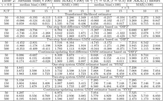
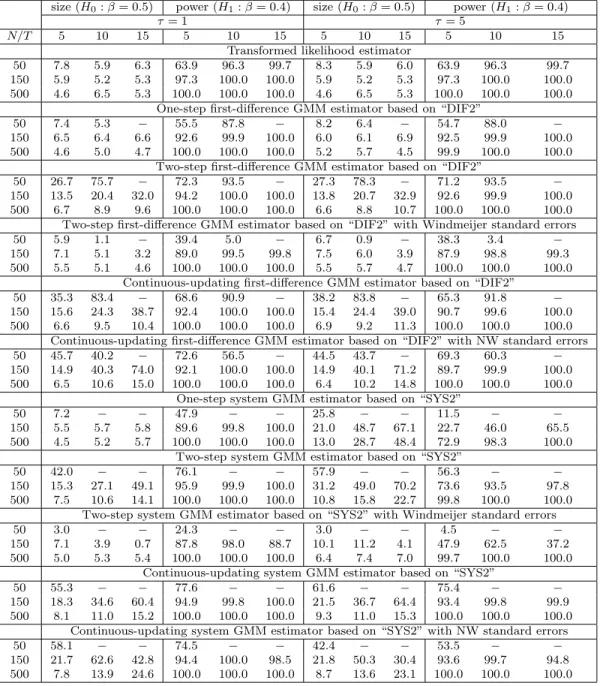
The small sample results for γ are summarized in Tables 1 to 4. Table 1 provides the results for the case of γ = 0.4, and shows that the transformed likelihood estimator has a smaller bias than the GMM estimators in all cases with the exception of the CU-GMM estimator (the last panel of Table 1). In terms of MAE the transformed likelihood estimator outperforms the GMM estimators in all cases.
As for the effect of increasing the variance ratio, τ, on the various estimators, we first recall that the transformed likelihood estimator must be invariant to the choice of τ, although the estimates reported in Table 1 do show some effects, albeit small. The observed impact of changes in τ on the performance of the transformed likelihood estimator is solely due to computational issues and reflects the dependence of the choice of initial values on τ in computation of the transformed ML estimators. One would expect that these initial value effects to disappear asN is increased, and this is seen to be the case from the results summarized in Table 1. In contrast, the performance of the GMM estimators deteriorates (in some case substantially) as τ is increased from 1 to 5. This tendency is especially evident in the case of the system GMM estimators, and is in sharp contrast to the performance of the transformed likelihood estimator which are robust to changes inτ. These observations also hold if we consider the experiments withγ = 0.9 (Table 2). Although the GMM estimators have smaller biases than the transformed likelihood estimator in a few cases, in terms of MAE, the transformed likelihood estimator performs best in all cases.
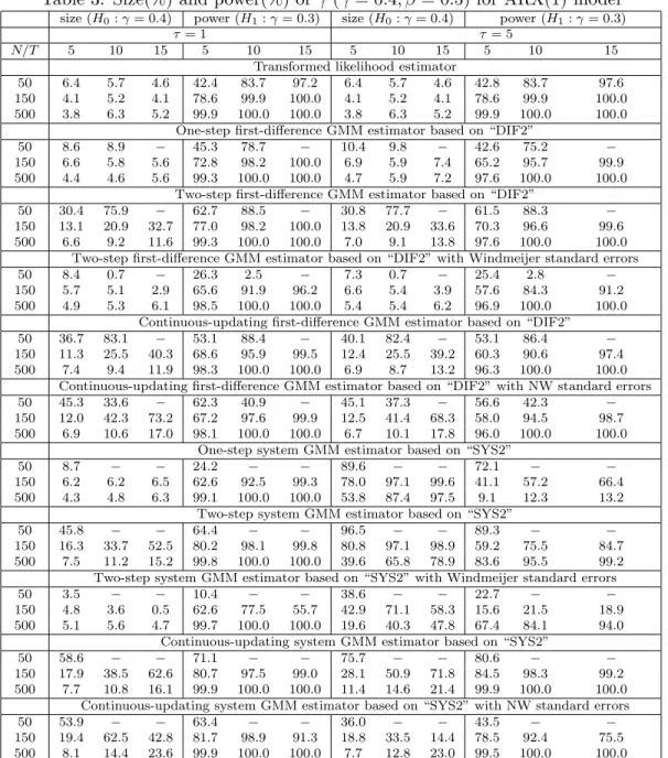
We next consider size and power of the various tests, summarized in Tables 3 and 4. Table 3 shows that the empirical size of the transformed likelihood estimator is close to the nominal size of 5% for all values ofT,N and τ.
For the GMM estimators, we find that the test sizes vary considerably depending onT,N,τ, the estimation method (1step, 2step, CU), and whether corrections are applied to the standard errors. In the case of the GMM results without standard error corrections, most of the GMM methods are subject to substantial size distortions whenN is small. For instance, whenN = 50,T = 5, andτ = 1, the size of the test based on DIF2(2step) estimator is 30.4%. But the size distortion gets smaller as
N increases. Increasing N to 500, reduces the size of this test to 6.6%. However, even with N = 500, the size distortion gets larger for two-step and CU-GMM estimators as T increases.
As to the effects of changes in τ on the estimators, we find that the system GMM estimators are significantly affected when τ is increased. When τ = 5, all the system GMM estimators have large size distortions even when T = 5 and N = 500,where conventional asymptotics are expected to work well. This may be due to large finite sample biases caused by a large τ.
Amongst the tests based on corrected GMM standard errors, Windmeijer (2005)’s correction seems to be quite useful, and in many cases it leads to accurate inference, although the corrections do not seem able to mitigate the size problem of the system GMM estimator when τ is large. The standard errors of Newey and Windmeijer (2009) are not always helpful, and although they improve the size property in some cases, they have either little effects or tend to worsen the test sizes in other cases.
Comparing power of the tests, we observe that the transformed likelihood estimator is in general more powerful than the GMM estimators. For example when N = 150, the transformed likelihood estimators have higher power than “SYS2(2stepW)” which is the most efficient amongst the reported
GMM estimators.
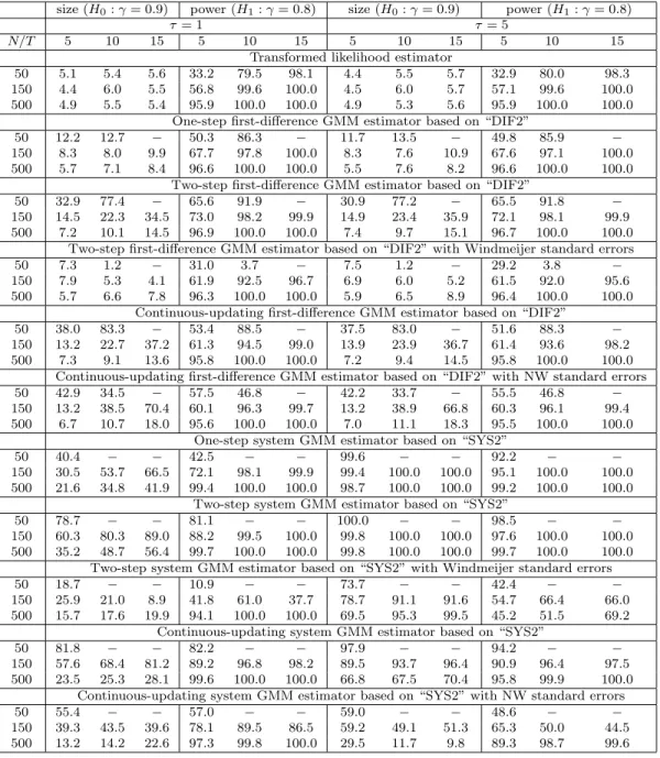
The above conclusions hold generally when we consider experiments with γ = 0.9 (Table 4), except that the system GMM estimators now perform rather poorly even for a relatively largeN. For example, when γ = 0.9, T = 5, N = 500 and τ = 1, size distortions of the system GMM estimators are substantial, as compared to the case where γ = 0.4. Although it is known that the system GMM estimators break down when τ is large8, the simulation results in Table 4 reveal that they perform poorly even whenτ is not so large (τ = 1).
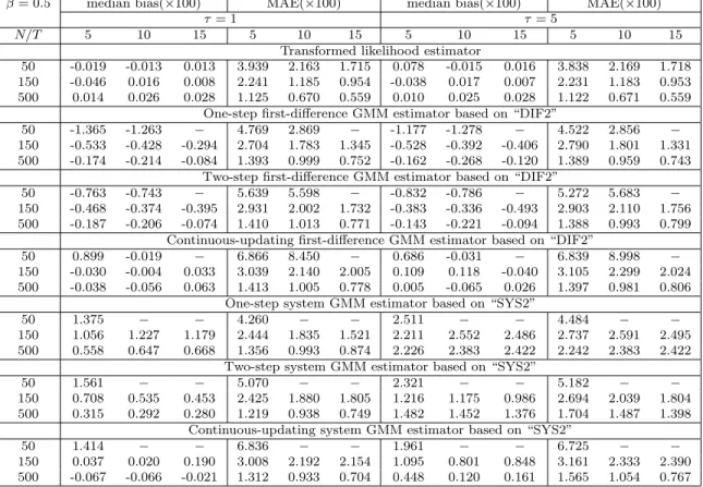
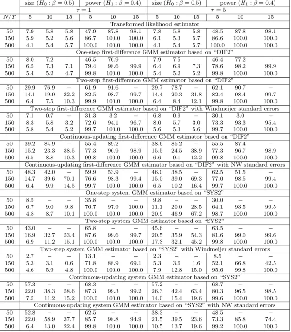
The small sample results for β (Tables 5 to 8), are similar to the results reported for γ. The transformed likelihood estimator tends to have smaller biases and MAEs than the GMM estimators in many cases, and there are almost no size distortions for all values ofT,N andτ. The performance of the GMM estimators crucially depends on the values ofT,N and τ. Unless N is large, the GMM estimators perform poorly and the system GMM estimators are subject to substantial size distortions when τ is large even forN = 500, although the magnitude of size distortions are somewhat smaller than those reported forγ.
The results for the long-run coefficient, δ =β/(1−γ), are reported in a supplementary appendix, and are very similar to those ofγ and β. Although the GMM estimators outperform the transformed likelihood estimator in some cases, in terms of MAE, the transformed likelihood estimator performs best in almost all cases. As for inference, the transformed likelihood estimator has correct sizes for all values of T, N and τ when γ = 0.4. However, it shows some size distortions when γ = 0.9 and the sample size is small, say, whenT = 5 andN = 50. However, size improves asT and/orN increase(s). When T = 15 and N = 500, there is essentially no size distortions. For the GMM estimators, it is observed that although the sizes are correct in some cases, say, the case with T = 5 and N = 500 when γ = 0.4, it is not the case whenγ = 0.9; even for the case ofT = 5 and N = 500, there are size distortions and a large τ aggravates the size distortions.
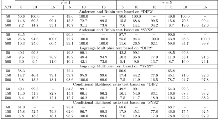
Finally, we consider weak instruments robust tests, which are reported in Tables 9 and 10. We find that test sizes are close to the nominal value only when T = 5 and N = 500. In other cases, especially when N is small and/orT is large, there are substantial size distortions. Although Newey and Windmeijer (2009) prove the validity of these tests under many weak moments asymptotics, they are essentially imposingm2/N → 0 or a stronger restriction where m is the number of moment con-ditions, which is unlikely to hold whenN is small and/orT is large. Therefore, the weak instruments robust tests are less appealing, considering the very satisfactory size properties of the transformed likelihood estimator, the difficulty of carrying out inference on subset of the parameters using the weak instruments robust tests, and large size distortions observed for these tests whenN is small.
In summary, for estimation of ARX panel data models the transformed likelihood estimator has
several favorable properties over the GMM estimators in that the transformed likelihood estimator generally performs better than the GMM estimators in terms of biases, MAEs, size and power, and unlike GMM estimators, it is not affected by the variance ratio of individual effects to disturbances.
5.2 AR(1) model
5.2.1 Monte Carlo design
The data generating process is the same as that in the previous section withβ = 0. More specifically,
yit are generated as
yit = αi+γyi,t−1+uit, fort= 1, ..., T and i= 1, ..., N, (38)
yi0 = αi 1−γ +ui0 √ 1 1−γ2, (39)
whereuit∼ N(0, σi2) withσi2 ∼ U[0.5,1.5]. Note thatyit are covariance stationary. Individual effects
are generated asαi =τ(qi−1)/
√
2 where qi∼χ21.
For parameters and sample sizes, we consider γ = 0.4,0.9, T = 5,10,15,20 N = 50,150,500,and
τ = 1,5.
Some comments on the computations are in order. For the starting value in the nonlinear opti-mization routine used to compute the transformed log-likelihood estimator, we use (eb,eγ,ω,e eσ2) where
eb = N−1∑Ni=1∆yi1, eγ is the one-step first-difference GMM estimator (21) where W˙ i and ˙Zi are
replaced with9 ˙ Wi= ∆yi1 .. . ∆yi,T−1 , Z˙i = yi0 0 0 yi1 yi0 0 yi2 yi1 yi0 .. . ... ...
yi,T−2 yi,T−3 yi,T−4
, e ω= [(N−1)eσu2]∑Ni=1 ( ∆yi1−eb )2 and eσu2 = [2N(T −2)]−1∑iN=1(∆yit−eγ∆yi,t−1)2.
For the first-difference GMM estimators, we consider two sets of moment conditions. The first set of moment conditions, denoted as “DIF1”, consists of E(yis∆uit) = 0 for s= 0, ..., t−2;t= 2, ..., T. In this case, the number of moment conditions are 10, 45, 105 for T = 5,10, 15, respectively. The second set of moment conditions, denoted by “DIF2”, consist of E(yi,t−2−l∆uit) = 0 with l = 0 for t = 2, and l = 0,1 for t = 3, ..., T. In this case, the number of moment conditions are 7, 17,27 for
T = 5,10,15, respectively.
Similarly, for the system GMM estimator, we add moment conditions E[∆yi,t−1(αi+uit)] = 0 for
t= 2, ..., T in addition to “DIF1” and “DIF2”, which are denoted as “SYS1” and “SYS2”, respectively.
9This type of estimator is considered in Bun and Kiviet (2006). Since the number of moment conditions are three,
this estimator is always computable for any values ofN andT considered in this paper. Also, since there are two more moments, we can expect that the first and second moments of the estimator to exist.
For the moment conditions “SYS1”, we have 14,54,119 moment conditions forT = 5,10,15, respec-tively, while for the moment conditions “SYS2”, we have 11, 26, 41 moment conditions for T = 5,
10,15, respectively. With regard to the inference, we use the robust standard errors formula given in Theorem 2 for the transformed log-likelihood estimator. For the GMM estimators, in addition to the conventional standard errors, we also compute Windmeijer (2005)’s standard errors for the two-step GMM estimators and Newey and Windmeijer (2009)’s standard errors for the CU-GMM estimators.
We report the median biases, median absolute errors (MAE), sizes (γ = 0.4 and 0.9) and powers (resp. γ = 0.3 and 0.8) with the nominal size set to 5%. As before, the number of replications is set to 1,000.
5.2.2 Results
As in the case of ARX(1) experiments, to save space, we report the results of the transformed likelihood estimator and the GMM estimators exploiting moment conditions “DIF2” and “SYS2”. Complete set of results are provided in a supplement, which is available upon request.
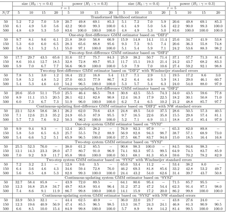
The biases and MAEs of the various estimators for the case of γ = 0.4 are summarized in Table 11. As can be seen from this table, the transformed likelihood estimator performs best (in terms of MAE) in almost all cases, the exceptions being the CU-GMM estimators that show smaller biases in some experiments. As to be expected, the one- and two-step GMM estimators deteriorate as the variance ratio,τ, is increased from 1 to 5, and this tendency is especially evident for the system GMM estimator. For the case ofγ = 0.9 (Table 12), we find that the system GMM estimators have smaller biases and MAEs than the transformed likelihood estimator in some cases. However, whenτ = 5, the transformed likelihood estimator outperforms the GMM estimators in all cases, both in terms of bias and MAE.
Consider now the size and power properties of the alternative procedures. The results for γ = 0.4 are summarized in Table 13. We first note that the transformed likelihood procedure shows almost correct sizes for all experiments. For the GMM estimators, although there are substantial size distortions when N = 50, the empirical sizes become close to the nominal value as N is increased. When T = 5,10 and N = 500 and τ = 1, the size distortions of the GMM estimators are small. However, when τ = 5, there are severe size distortions for the system GMM estimator even when
N = 500. For the effects of corrected standard errors, similar results to the ARX(1) case are obtained. Namely, Windmeijer (2005)’s correction is quite useful, and in many cases it leads to accurate inference although the corrections do result in severely under-sized tests in some cases. Also, this correction does not seem that helpful in mitigating the size problem of the system GMM estimator when τ is large. The standard errors of Newey and Windmeijer (2009) used for the CU-GMM estimators are not always helpful: although they improve the size property in some cases, they have almost no effects in some cases or worsen the test sizes in other cases.
Size and power of the tests in the case of experiments with γ = 0.9 are summarized in Table 14, and show significant size distortions in many cases. The size distortion of the transformed likelihood
gets reduced for relatively large sample sizes and its size declines to 7.7% when τ = 1, N >150 and
T > 15. As to be expected, increasing the variance ratio, τ, to 5, does not change this result. A similar pattern can also be seen in the case of GMM-DIF estimators if we considerτ = 1. But the size results are much less encouraging if we consider the system GMM estimators. Also, as to be expected, size distortions of GMM type estimators become much more pronounced when the variance ratio is increased toτ = 5.
Finally, we consider the small sample performance of the weak instruments robust tests which are provided in a supplement, to save space. These results show that size distortions are reduced only whenN is large (N = 500). In general, size distortions of these tests get worse asT, or the number of moment conditions, increases. In terms of power, although “LM(SYS2)” and “CLR(SYS2)” tests have almost the same power as the transformed likelihood estimator when γ = 0.4, T = 5, N = 500 and
τ = 1, their powers decline whenτ = 5,unlike the transformed likelihood estimator which is invariant to changes in τ. For the case of γ = 0.9, the results are very similar to the case of γ = 0.4. Size distortions are small only when N is large. When N is small, there are substantial size distortions.
6
Concluding remarks
In this paper, we proposed the transformed likelihood approach to estimation and inference in dynamic panel data models with cross-sectionally heteroskedastic errors. It is shown that the transformed likelihood estimator by Hsiao et al. (2002) continues to be consistent and asymptotically normally distributed, but the covariance matrix of the transformed likelihood estimators must be adjusted to allow for the cross-sectional heteroskedasticity. By means of Monte Carlo simulations, we investigated the finite sample performance of the transformed likelihood estimator and compared it with a range of GMM estimators. Simulation results revealed that the transformed likelihood estimator for an ARX(1) model with a single exogenous regressor has very small bias and accurate size property, and in most cases outperformed GMM estimators, whose small sample properties vary considerably across parameter values (γ and β), the choice of moment conditions, and the value of the variance ratio, τ.
In this paper,xitis assumed to be strictly exogenous. However, in practice, the regressors may be endogenous or weakly exogenous (c.f. Keane and Runkle, 1992). To allow for endogenous and weakly exogenous variables, one could consider extending the panel VAR approach advanced in Binder et al. (2005) to allow for cross-sectional heteroskedasticity. More specifically, consider the following bivariate model:
yit = αyi+γyi,t−1+βxit+uit
xit = αxi+ϕyi,t−1+ρxi,t−1+vit
ifθ= 0, and endogenous ifθ̸= 0. This model can be written as a PVAR(1) model as follows ( yit xit ) = ( αyi+βαxi αxi ) + ( γ+βϕ βρ ϕ ρ ) ( yi,t−1 xi,t−1 ) + ( uit+βvit vit ) ,
for i= 1,2, ..., N. Let A ={aij}(i, j = 1,2) be the coefficient matrix of (yi,t−1, xi,t−1)′ in the above
VAR model. Then, we have β = a12/a22, γ = a11−a12a21/a22, ρ = a22 and ϕ = a21. Thus, if we
estimate a PVAR model in (yit, xit), allowing for fixed effects and cross-sectional heteroskedasticity, we can recover the parameters of interest, γ and β, from the estimated coefficients of such a PVAR model. However, detailed analysis of such a model is beyond the scope of the present paper and is left to future research.
A
Proofs
A.1 Preliminary results
In this appendix we provide some definitions and results useful for the derivations in the paper. Lemma A1 Let Ωbe given by (8). Then the determinant and inverse of Ωare:
|Ω| = g= 1 +T(ω−1), (40) Ω−1 = g−1 T T −1 ... 2 1 T −1 (T−1)ω ... 2ω ω T −2 2 2ω 2 [(T −2)ω−(T −3)] (T−2)ω−(T−3) 1 ω ... (T−2)ω−(T−3) (T−1)ω−(T−2) .
The generic(t, s)th element of the(T−1)×(T−1)lower block ofΩ−1, denoted byΩe, can be calculated using the following formulas, fort, s= 1,2, ..., T−1:
{ e Ω } ts = { s(T−t)ω−(s−1) (T −t), (s≤t) t(T −s)ω−(t−1) (T−s), (s > t) . (41) Proof. See Hsiao et al. (2002).
Lemma A2 Let Φbe defined in (10). We have
where ϑ′= (T, T −1, . . . ,2,1)and
tr(ΦΩ) =tr(ϑϑ′Ω)=ϑ′Ωϑ=T g, (42)
where g is given by (40).
Proof. See Hsiao et al. (2002).
Lemma A3 Let {xi, i = 1,2, ..., N} and {zi, i = 1,2, ..., N} be two sequences of independently dis-tributed random variables, such that xizi are independently distributed across i, although xi and zi
need not be independently distributed of each other. Then
E [( N ∑ i=1 xi ) ( N ∑ i=1 zi )] = N ∑ i=1 Cov(xi, zi) + [ N ∑ i=1 E(xi) ] [ N ∑ i=1 E(zi) ] .
Lemma A4 Consider the transformed model (7). Under Assumptions 1 and 2 we have
E(∆W′iΩ−1ri
)
=0, (i= 1,2, ..., N), (43)
where Ω is given in (8). Further,
E(r′iΦ∆Wi ) = ( 0 0 ϖ 0 ) , (i= 1,2, ..., N), (44)
where Φ is given by (10), and ϖ̸= 0.
Proof. Let ∆yei,−1 = (0,∆yi1, ...,∆yi,T−1)′ and note that, for (43) to hold, it is only needed to prove
thatE
(
∆ey′i,−1Ω−1r
i
)
=0. To show this, letpi=Ω−1r
i = (pi1, ..., piT)′ where by (41) pi1 = T vi1+ T ∑ s=2 (T −s+ 1)∆uis, pit = (T −t+ 1)vi1+ t ∑ s=2 hts∆uis+ T ∑ s=t+1 kts∆uis, (t= 2, ..., T −1) piT = vi1+ T ∑ s=2 hT s∆uis and hts = (T −t+ 1) [(s−1)ω−(s−2)], (45) kts = (T−s+ 1) [(t−1)ω−(t−2)].
Then, we have E[∆ey′i,−1Ω−1ri ] = T ∑ t=2 E[pit∆yi,t−1] = T∑−1 t=2 E[pit∆yi,t−1] +E[piT∆yi,T−1] = T∑−1 t=2 E [ (T −t+ 1)vi1∆yi,t−1+ t ∑ s=2 hts∆uis∆yi,t−1+ T ∑ s=t+1 ks∆uis∆yi,t−1 ] +E(piT∆yi,T−1) = T ∑ t=2 (T−t+ 1)E(vi1∆yi,t−1) + T ∑ t=2 t ∑ s=2 htsE(∆uis∆yi,t−1) = A1+A2.
where we used E(∆uis∆yit) = 0 for t < s−1. To deriveA1 and A2, we use the followings10:
σi−2E(vi1∆yit) = { ω t= 1 γt−2(γω−1) t= 2, ..., T (46) σ−i 2E(∆uis∆yit) = −1 t=s−1 (2−γ) s=t −(1−γ)2γt−s−1 s < t (47)
Using (46) and (47), we have
A1 = σ2i [ (T −1)ω+ (γω−1) T ∑ t=3 (T −t+ 1)γt−3 ] , (48) 10
These results are obtained by noting that ∆yit can be written as follows
∆yi1 = b+π′∆xi+vi1, ∆yit = γt−1∆yi1+β (t−2 ∑ j=0 γjxi,t−j ) + t−2 ∑ j=0 γj∆ui,t−j = γt−1(b+π′∆xi ) +γt−1vi1+β (t−2 ∑ j=0 γjxi,t−j ) + t−2 ∑ j=0 γj∆ui,t−j, (t= 2, ..., T).