Using High Resolution X-ray Computed Tomography to
Create an Image Based Model of a Lymph Node
L. J. Coopera,∗, B. Zeller-Plumhoffa, G. F. Cloughb, B. Ganapathisubramania,
T. Roosea
aFaculty of Engineering and the Environment, University of Southampton, Highfield
Campus, Southampton, SO17 1BJ, UK
bFaculty of Medicine, University of Southampton, Southampton General Hospital,
Southampton, SO16 6YD, UK
Abstract
Lymph nodes are an important part of the immune system. They filter the lymphatic fluid as it is transported from the tissues before being returned to the blood stream. The fluid flow through the nodes influences the behaviour of the immune cells that gather within the nodes and the structure of the node itself. Measuring the fluid flow in lymph nodes experimentally is challenging due to their small size and fragility. In this paper, we present high resolution X-ray computed tomography images of a murine lymph node. The impact of the resulting visualized structures on fluid transport are investigated using an image based model. The high contrast between different structures within the lymph node provided by phase contrast X-ray computed tomography reconstruction results in images that, when related to the permeability of the lymph node tissue, suggest an increased fluid velocity through the interstitial channels in the lymph node tissue. Fluid taking a direct path from the afferent to the efferent lymphatic vessel, through the centre of the node, moved faster than the fluid that flowed around the periphery of the lymph node. This is a possible mechanism for particles being moved into the cortex.
Keywords: Lymphatic System, Image based modelling, Porous media
∗Corresponding author
1. Introduction
Lymph nodes are a site for immune cell transfer between blood and lym-phatic fluid, where antigen sensing and immune cell activation takes place. Lymph nodes have been imaged using histology for many years [1, 2, 3, 4]. However, histology can only ever give 2D structural information about this 3D 5
organ. Some of the structures identified within the lymph nodes are:
• a fibrous outer capsule encasing the whole node
• a low resistance pathway for fluid just under the capsule, known as the subcapsular sinus;
• an area of dense lymphoid tissue, called the cortex; 10
• and the when the fluid leaves the cortex and subcapsular sinus, if it is not reabsorbed via the blood vessels, it enters the medullary sinuses before exiting the node through an efferent lymphatic vessel.
The structure of lymph nodes can be used to theorise on the behaviour of fluid flow through the nodes [5]. The fluid flow in lymph nodes has been shown to 15
affect the arrangement of the reticular cell network [6] and to influence the mi-gration of immune cells [7, 8]. The fluid flow also determines the concentration of proteins in the lymphatic fluid [9, 10, 11]. Understanding the pathways of fluid flow through the nodes will contribute to our knowledge of immune cell migration, development of lymph node structures, protein transfer and cancer 20
metastasis [12]. Experimental investigations of fluid flow through lymph nodes is challenging due to the lymph node’s small size and fragility. In this paper, we combine high resolution imaging with computational modelling to demon-strate how the internal structures within the node can influence the fluid flow pathways.
25
Mayer et al. [13] used selective plane illumination microscopy (SPIM) to visualise the high endothelial venules and dendritic cells in two lymph nodes in 3D. The SPIM images of these lymph nodes have also been used to create a
finite element model of fluid flow through lymph nodes [14]. The model based on the SPIM images was used to estimate properties such as the permeability 30
of the node by fitting to experimental data and showed that the main pathway for fluid flow in the model was through the centre of the node. A limitation of using SPIM images is that fluorescent staining is required to enhance the image contrast of the structures within the node. One consequence of this is that the relation between the permeability of the lymph node tissue and the greyscale of 35
the image may be biased depending on the diffusion of the stain into the tissue. For example, there could be more stain around the outer edges of the node than in the centre.
Other three-dimensional, non-destructive imaging methods exist that do not require soft tissue to be stained to generate image contrast, and thus overcome 40
the limitation of using SPIM images. Namely, high resolution X-ray computed tomography (CT) can be used to visualise the variable density of the lymph node internal tissue structure in 3D. The capability of synchrotron radiation CT has previously been used to generate 3D data sets of soft tissue for subsequent finite element modelling. This is demonstrated by Zeller-Plumhoff et al. [15, 16] in 45
the context of oxygen diffusion in murine muscle. High resolution CT can also enable the analysis of morphological measures in biological systems and their functional importance [16].
In this paper, we use X-ray CT images with the finite element method to create an image based model of fluid flow through a lymph node. We are 50
utilising the relationship between image greyscale and tissue permeability to assess the importance of the structures observed using X-ray CT on lymphatic fluid flow. Two different methods of enhancing image contrast for soft tissue features are used in order to establish which method best enables visualisation of the features of interest. These methods are edge enhancement by direct 55
image reconstruction using the fast reconstruction algorithmGridrec[17, 18] and phase retrieval with the Paganin single-distance non-iterative phase retrieval algorithm [19] and subsequent reconstruction withGridrec. The outcome from the phase retrieval images produces results that are consistent with previous
studies on the internal structure of the node [5]. The methodology presented 60
in this paper can be generalised and used to assess differences between lymph nodes due to, for example, different stages of a disease.
2. Methods
2.1. Sample Preparation, Imaging and Reconstruction
All animal procedures were in accordance with the regulations of the United 65
Kingdom Animals (Scientific Procedures) Act 1986 and were conducted un-der Home Office Licence number 70-6457. The study received institutional approval from the University of Southampton Biomedical Research Facility Re-search Ethics Committee. The mouse was maintained under controlled condi-tions and at 15 weeks of age, the mouse was sacrificed by cervical dislocation. A 70
mesenteric lymph node (≈1 x 1 x 2 mm3) was dissected from a male C57BL/6
mouse, fixed in formalin, dehydrated in methylated spirit and embedded in paraffin wax. The lymph node was scanned at the beamline for Tomographic Microscopy and Coherent radiology experiments (TOMCAT) at the Swiss Light Source, Villigen, Switzerland. The imaging was carried out using an energy of 75
14 keV, using a propagation distance between sample and detector of 60 mm. The exposure time was 180 ms and 1601 projections were taken over 180◦(with
additional 32 dark field and 160 flat field images). The resulting voxel size was (0.65µm)3. The images were reconstructed using two methods, both in-house
implementations at TOMCAT: theGridrecalgorithm [17, 18] and thePaganin
80
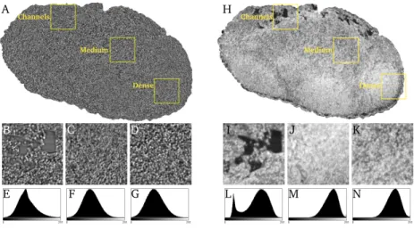
phase retrieval algorithm [19] withGridrec. A comparison of the two resulting reconstructions can be seen in figure 1. The edge enhancement in the direct
Gridrecreconstruction shows small length scale features within the node, which could possibly be the lymphocytes that make up the tissue of the node. The higher contrast of thePaganinreconstruction shows features at the larger length 85
scale. It is possible to distinguish structures that appear to be B cell follicles, lymphatic channels, the dense cortex and less dense paracortex, similar to those seen with histology, e.g. [3]. It should be noted that although structures can be
Channels Dense Medium A B C D E F G Channels Dense Medium H I J K L M N
Figure 1: Different regions used to evaluate the effect of areas of the node on the flow pathways in the model for A)Gridrecreconstruction and H)Paganinreconstruction. B and I) Channels
fromGridrecandPaganin, respectively; C and J) Dense fromGridrecandPaganin,
respec-tively; D and K), Medium fromGridrec andPaganin, respectively; E and L), Histogram of channels forGridrecandPaganin, respectively; F and M), Histogram of dense forGridrecand
Paganin, respectively; G and N), Histogram of medium forGridrecandPaganin, respectively.
The squares are all 0.13 mm2.
distinguished due to the contrast of the X-ray CT images, it would be necessary to correlate these images with histology to confirm the identity of these struc-90
tures. Histology was not undertaken as correlating the 2D histological sections to the 3D image stacks would have required an extra layer of techniques to be applied, trialled and calibrated, that are outside the scope of this paper.
2.2. Blood Vessel Segmentation and Construction
Only a proportion of blood vessels appeared visible in the X-ray CT recon-95
structions. Therefore a vascular tree was constructed computationally. The blood vessels that could be visualised were segmented manually using the magic wand tool on individual slices spaced 5-10 µm apart in Avizo Fire 9.0 (FEI, Hillsboro, OR, USA). Interpolation between the manually segmented slices was used to create continuous blood vessels. The blood vessels were constructed 100
computationally. The vessels that could be segmented out were used as inputs to the fractal L-system algorithm used to create the vascular network. Details of the L-system used can be found in Appendix A.
The tree was generated using a script in MATLAB and converted into an image stack using macros in Fiji image analysis software [20]. A new tree was 105
initiated at the end points of each segmented branch from the images. The 3D line tool from the 3D tool plugin was used to draw white lines of a fixed radius on a stack of black images. The macro could then be run in Fiji to create an image stack of the computationally created blood vessels that was then combined with the masks for the surfaces representing the lymphatic vessel connections and the 110
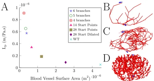
mask for the outline of the lymph node. Three separate tree realisations were created consisting of 4, 5 and 6 levels of branches, respectively, with heading vectors based on the segmented images. Another three trees were created by defining start points and heading vectors randomly. Two of these trees were created with 14 and 28 start points, respectively, and 6 branching levels. All 115
vessels created in these trees had a diameter of 5.2 µm. The sixth tree was the 28 start point tree where the diameter of the vessels were increased to 10.4 µm. The value ofLp for each model was calculated from the published value
ofLp×S for the WT node from [14], whereS is the blood vessel surface area,
by dividing by the surface area for the created blood vessel trees. The models 120
with different branching structures were modelled with a constant permeability for the lymph node interstitial space. The value ofLp for each tree can be seen
in figure 2.
2.3. Image Processing
The X-ray CT scans of the node were processed as follows. The whole lymph 125
node was segmented by applying a threshold to the phase contrast image stack. The threshold was chosen by manually varying the minimum and maximum values of the histogram so that the whole node was segmented and the back-ground colour was set to black. Any additional material, mainly fatty tissue around the node, was removed from the image manually. The voxel size was 130
A
B
C
D
0 1 2 3 4 ·10−6 0 0.2 0.4 0.6 0.8 1 ·10− 6Blood Vessel Surface Area (m2) Lp (m/P a.s) 6 branches 5 branches 4 branches 14 Start Points 28 Start Points 28 Start Dilated WT
Figure 2: A) Relationship of blood vessel surface area to the value ofLp, where the value of
LpS= 2.27×10⁻¹³has been assumed and is represented by WT based on the wild type node
from Cooper et al. [14]. Figures B and C show examples of the blood vessel networks used corresponding to 4 branches and 28 Start Points, respectively. The blood vessels are shown in red and the positions of the afferent and efferent lymphatics in blue, with the afferent vessel at the top of the image and the efferent vessel at the bottom. Figure D shows the high endothelial venules for the wild type (WT) node from Cooper et al. [14] for comparison.
binned to (1.3µm)3 to decrease the size of the image stack to an eighth of the
original to reduce the computational resources required. A mask was created of the segmented node, i.e. a binary image that showed the lymph node geometry without the internal detail. The mask was used to remove everything outside of the node from theGridrec image stack, so that the node was on a white back-135
ground, as shown in figure 1A and figure 1H. Each slice fromGridrecand phase contrast image stacks were saved as .png files for use in COMSOL 4.4 (COM-SOL AB, Sweden). The mask of the computationally created blood vessels was subtracted from the mask of the segmented node, creating binary images that showed the blood vessels as holes within the mask of the node geometry. To 140
segment the afferent and efferent lymphatic vessels the magic wand tool was used in Avizo Fire on the segmented phase stack. This was saved as another mask. The masks of the segmented node with blood vessels and the mask of
the afferent and efferent lymphatic vessels were imported into ScanIP 4.0 (Sim-pleware Ltd, UK) for meshing. The whole node was meshed with minimum 145
element size 2.25 µm and maximum element size 9µm. The mesh produced had the geometry of the lymph node with holes that represented the location of blood vessels. A more detailed description of how to use ScanIP to mesh the lymph node can be found in [14].
2.4. Modelling of Fluid Flow Through the Lymph Node
150
The modelling was carried out following the approach first introduced in Cooper et al. [14]. Briefly, the fluid flow through the lymph node interstitium, Ω, is modelled using Darcy’s law in combination with the fluid conservation equation, u=−κ µ∇p, x∈Ω C,ΩL (1) ∇ ·u= 0, x∈ΩC,ΩL (2) whereκis the interstitial permeability defined using the image stacks,
κ= (−k0im1(x, y) +k1)×(z <1.3µm)
+ (−k0im2(x, y) +k1)×(z≥1.3µm)×(z <2.6µm) (3)
+· · ·+ (−k0imn(x, y) +k1)×(z≥1.3 (n−1)µm), x∈ΩC,ΩL
wherek0andk1relate the grey scales of the images and the permeability linearly.
imnis the nth slice of the image stack,x,yandzand the coordinates of the point
in the image stack. Here,k0= 6.2086×10⁻¹¹ m2 andk1= 6.2096×10⁻¹¹ m2,
the values are for the wild type murine lymph node after Cooper et al. [14] unless otherwise stated. uis the fluid velocity,µ= 0.0015 Pa·s is the dynamic viscosity 155
of the lymphatic fluid [21] andpis the fluid pressure in the node interstitium. The boundary condition on the blood vessel surfaces was defined using Star-ling’s principle,
ˆ
where ˆnb is the vector normal pointing from the surface of the blood vessels
toward the interstitum,ρ= 1000 kg/m3is the density of the fluid,L
p(m/Pa·s)
is the hydraulic conductivity of the blood vessel walls and had different values depending on the surface area of the blood vessel tree, pv = 973 Pa is the 160
pressure inside the blood vessels [11],σ= 0.9 (no units) is the osmotic reflection coefficient [22], and ∆π=πv−πn= 341 Pa, whereπv(Pa) is the plasma colloid
osmotic pressure in the blood vessels andπn (Pa) is the node colloid osmotic
pressure. The value of ∆π= 341 Pa was found by fitting the wild type model in Cooper et al. [14] to experimental data. This value is smaller than was 165
approximated by Adair and Guyton [11], ∆π≈2080 Pa for dog lymph nodes, and the value measured in the skin of mice ∆π ≈ 1500 Pa [23]. However, it was found that a higher value of ∆πdid not give efferent flow rates that fit well with the experimental data [14]. ΓL
b is the blood vessel boundary.
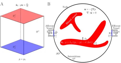
In this paper we present two studies; firstly, a mesh density study to optimise the accuracy of the model result while reducing the computational resources re-quired. For this study a cubic subsection of the lymph node is used to reduce the complexity of the model until the mesh parameters have been established. Secondly, we present a study where the whole lymph node is modelled to in-vestigate how the internal structure of the node affects the pathways of fluid through the node. One side of the cube, Λ1, has the boundary condition,
ˆ
n1·ρu= F1
A1
, x∈ΓC1, (5)
where ˆn1 is the vector normal on the side of the cube pointing into the body of
the cube,F1 (kg/s) is the flow rate through this side of the cube andA1 (m2)
is the area of Λ1. On the opposite side of the cube, Λ2 the pressure is fixed,
p=p2, x∈ΓC2, (6)
wherep2 (Pa) is a fixed pressure value. A no-flux condition was applied to all
other boundaries. These conditions are summarised in figure 3A. For the whole lymph node model the condition of afferent lymphatic boundary, Γa, was
ˆ na·ρu= Fa Aa , x∈ΓL a, (7)
p=p2 ˆ n1·ρu=FA11 ΓC 1 ΓC 2 ΩC Afferent Vessel Inlet Fa Node Efferent Vessel Outlet pe ˆ na ΓL a ΓLe ˆ nb ΓL b Interstitium ΩL ∂ΩL u u u=−κ µ∇p ∇ ·uuu= 0 ˆ n n nb·ρ=Lp((pv−p)−σ(∆π)) Blo od vessel
A
B
Figure 3: Sketch summarising the cube and whole lymph node models. Dashed black lines show position of afferent and efferent vessels, although these are not modelled. The arrows labelled with ˆnshow the positive normal vector to the boundaries.
where ˆnais the vector normal to the afferent lymphatic boundary, pointing into
the lymph node, Fa (kg/s) is the afferent flow rate and Aa (m2) is the area
of the afferent lymphatic boundary. The pressure is fixed tope on the efferent
lymphatic boundary, Γe,
p=pe, x∈ΓLe. (8)
The whole node model is summarised in figure 3B. 170
2.5. Mesh Density Study
There are some computational choices that needed to be made with regards to how the model is solved numerically, i.e., size of the mesh elements, voxel size of the images and the histogram of the grey scales of the images. To explore the error resulting from these choices, a representative subvolume from the image 175
stack of the whole node was used. This cube was chosen so that it contained one branch of a blood vessel and was 130µm×130µm×130µm. Using a subsection of the volume reduced the amount of computational resources required. An inlet flow rate ofF1= 5.1×10⁻⁴m/s was applied to the upper face of the cube and
an outlet pressure ofp2 = 204 Pa was defined on the lower face. These values
were evaluated from the two planes 130µm apart through the wild type (WT) node model in Cooper et al. [14].
Two parameters were defined: ∆y, which had a constant value of 2.25 µm (√3×1.32 µm) based on the voxel size of the images; and ∆x the maximum
size of the mesh elements. Initially ∆xwas equal to the minimum element edge 185
length, 2.25µm and then increased by a factor of two six times. This resulted in ∆x
∆y = 32, 16, 8, 4, 2 and 1.
2.6. Region Study of Selected Node Structures
A further study was conducted to investigate the effect of different structures within the node, such as lymphatic channels and varying density within the 190
cortex. Three different regions were used. The regions are highlighted in figure 1. The first region of interest was chosen from an area containing channels, i.e. area with no lymphatic tissue, to be known as ‘Channels’, figure 1B and 1I forGridrec
andPaganin, respectively. The second region was from a densely packed area, known as ‘Dense’, 1C and 1J forGridrec andPaganin, respectively. The third 195
region represented the area from the centre of the node, to be called ‘Medium’, figure 1D and 1K for Gridrec and Paganin, respectively. The corresponding histograms of the stacks from the Gridrec and Paganin image stacks are also shown in figure 1.
The results from the mesh density and region studies were used to determine 200
which mesh element size should be used to model the whole node and whether to use theGridrec or Paganin reconstructed image stack. The results of these studies are presented in sections 3.1 and 3.2
2.7. Whole Lymph Node Model
The whole node model was calculated using a constant value for the per-205
meability, for six models with the same external geometry, but with different geometries of blood vessels with different surface areas. This was to investi-gate the effect of different blood vessel geometries on the pathways of fluid flow through the lymph node. The afferent lymph flow rate was defined as
Fa = 7.6×10⁻⁷ kg/s [11]. The efferent lymph pressure was set tope= 0 Pa, 210
i.e. everything was measured against atmospheric gauge pressure.
The geometry with 6 branches was used to create a model where the per-meability was defined by the images in the Paganin image stack. This was compared to the constant permeability model, with the same blood vessel ge-ometry, to see how the variable permeability affected the flow pathways within 215
the lymph node.
3. Results
3.1. Mesh Density Study
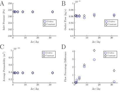
The results of the mesh density study are shown in figure 4. The ratio of the
A
B
C
D
0 10 20 30 240 242 244 246 248 250 ∆x/∆y Inlet Pressure (P a) Gridrec Constant 0 10 20 30 0.9 0.92 0.94 0.96 0.98 1·10−8 ∆x/∆y Outlet Flo w (kg/s) Gridrec Constant 0 10 20 30 0.2 0.4 0.6 0.8 1·10− 10 ∆x/∆y Av erage P ermeabilit y (m 2) Gridrec Constant 0 10 20 30 0 1 2 3 4 ∆x/∆y Flo w P ercen tage Difference Gridrec ConstantFigure 4: Results of different mesh densities and image stack histograms. A) Inlet; B) Outlet; C) Permeability; D) Flux through central plane.
mesh density to the voxel size, ∆x/∆y, did not have a significant effect on the 220
inlet pressure or outlet flow results. However the midplane flow, figure 4d, is affected. The difference between the mesh with ratio ∆x/∆y=4 and the finest mesh have a difference of less than 1% for the flux through the central plane,
i.e. well below any experimental error associated with biomedical experiments in this field. Therefore it is suitable to use ∆x/∆y = 4 for further model 225
simulations presented in this paper.
3.2. Region Study of Selected Node Structures
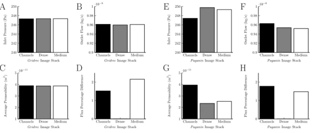
Taking image stacks from different areas of the Gridrecimages of the node did not result in much variation for the inlet pressure, outlet pressure or average permeability, figure 5A, B and C. It did not have the expected effect on the
A B
C D
Channels Dense Medium 240 242 244 246 248 250
GridrecImage Stack
Inlet
Pressure
(P
a)
Channels Dense Medium 0.9 0.92 0.94 0.96 0.98 1·10−8
GridrecImage Stack
Outlet
Flo
w
(kg/s)
Channels Dense Medium 1 2 3 4 5·10− 11
GridrecImage Stack
Av erage P ermeabilit y (m 2)
Channels Dense Medium 0
1 2
GridrecImage Stack
Flux P ercen tage Difference E F G H
Channels Dense Medium 240 242 244 246 248 250
PaganinImage Stack
Inlet
Pressure
(P
a)
Channels Dense Medium 0.9 0.92 0.94 0.96 0.98 1·10−8
PaganinImage Stack
Outlet
Flo
w
(kg/s)
Channels Dense Medium 1 2 3 4 5·10− 11
PaganinImage Stack
Av erage P ermeabilit y (m 2)
Channels Dense Medium 0
1 2
PaganinImage Stack
Flux
P
ercen
tage
Difference
Figure 5: Graphs show how using the image stacks from different regions of the node from the Gridrec andPaganinreconstructions, which were used to define the permeability, affected the flow in a subsection of the node. A and E) Inlet forGridrecandPaganinreconstructions, respectively; B and F) Outlet forGridrecandPaganinreconstructions, respectively; C and G) Permeability forGridrecandPaganin reconstructions, respectively; D and H) Flux through central plane forGridrecand Paganin reconstructions, respectively. For theGridrec image stack, the inlet, outlet and average permeability are not affected, but the flux percentage difference is. For thePaganin image stack, the inlet, outlet, average permeability and flux percentage difference are all affected.
230
central cut plane, shown in figure 5D. It was expected that the ‘Channels’ image stack would allow more flux through than the ‘Medium’ and ‘Dense’ stacks, but the results show more flux through the ‘Medium’ stack. This is probably a result of the very similar grey scale histograms for the image stacks, figures 1E, F and G. It appears that the grey scale of the ‘Channels’ does not distinguish 235
Taking stacks from different areas of thePaganin image stack of the node resulted in comparatively more variation for the inlet pressure, outlet pressure, and average permeability, figure 5E, F and G. It affected the flow percentage difference through the central cut plane as was expected, see figure 5H, with the 240
most flow though the ‘Channels’ image stack. The histogram for the Paganin
‘Channels’ image stack, figure 1l, clearly shows two peaks, one which represents the grey scale of the channels, and the other the grey scale of the surrounding lymphatic tissue.
3.3. Whole Lymph Node Model
245
The whole node model was calculated using a constant value for the perme-ability for six model set-ups with different blood vessel geometries. Figure 6A, shows how that inlet pressure increased as the surface area of the blood vessels increased. As the surface area of the blood vessel network increases so does the
·10−6
A
B
0 1 2 3 4 6 7 8·10−7Vessel Surface Area (m2)
Outlet Flo w Rate (kg/s) 6 branches 5 branches 4 branches 14 Start Points 28 Start Points 28 Start Dilated WT ·10−6 0 1 2 3 4 300 320 340 360 380
Vessel Surface Area (m2)
Inlet Pressure (P a) 6 branches 5 branches 4 branches 14 Start Points 28 Start Points 28 Start Dilated WT
Figure 6: Results showing how the surface area of the blood vessels affects the inlet and outlet flow conditions. A) Inlet pressure; B) Outlet flow rate.
volume. This reduces the cross-sectional area perpendicular to the flow, which 250
effectively increase the overall resistance of the lymph node and therefore in-creases the afferent pressure required to maintain the outlet flow rate. In figure 6B, the outlet flow rate is similar for all the blood vessel surface areas. The global value for Lp is varied for each model so that all the models have the
same outlet flow rate even through the surface area of the blood vessel network 255
changes.
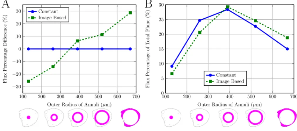
To compare the differences between the constant and variable permeability models, the flux through a plane equidistant between the inlet and outlet was evaluated. Figure 7A shows that the model which used the image based perme-ability causes more flow around the outer sections of the node than the constant 260
permeability. The high density material in the middle of the node is causing the
A
100 200 300 400 500 600 700 −30 −20 −10 0 10 20 30Outer Radius of Annuli (µm)
Flux P erce n tage Difference (%) Constant Image Based
B
100 200 300 400 500 600 700 0 5 10 15 20 25 30Outer Radius of Annuli (µm)
Flux P ercen tage of T otal Plane (%) Constant Image Based
Figure 7: Comparing flux through different annuli (shown in images below graph) through 2D plane equidistant between the inlet and outlet. A) Flux percentage difference through annuli. Values normalised to constant permeability results for comparison, thus all constant values are 0. B) Percentage of the total flux through the plane that passes through each annuli.
flow to take less resistant paths further out. Figure 7B shows the percentage of the total flux through the plane that passes through each annuli. This shows that the annuli with the highest percentage of flux is the middle annuli with an outer radius 390µm. These results show that incorporating the image based 265
permeability into the model does not cause the majority of the flow to pass around the outer edge of the node, which would be expected if the subcapsular sinus is considered as the path of least resistance. This could indicate the lymph node has shrunk due to the process of fixation and, therefore, the subcapsular sinus has not been fully visualised by the X-ray CT imaging.
270
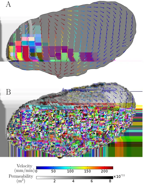
between the two models in a plane perpendicular to the inlet and the outlet. The direction and general flow morphology is similar, but that the velocity of the flow is different. The effect of the inlet and outlet can clearly be seen in the flow velocity in the image from the constant permeability model, figure 8A. The 275
fastest flow takes a direct path between the inlet and the outlet. The image based permeability model similarly shows the majority of the fast flow taking a direct path between the inlet and the outlet but there are some small areas of slower velocities where there is more resistance to the flow due to the variable permeability, figure 8B.
280
In planes parallel to that shown in figure 8, but further from the inlet and outlet, the flow is slower. It is possible to see in the image based permeability model, that near the upper surface, where there are dark areas, the flow is faster than in the same area in the constant permeability model. A similar phenomenon can be observed in the lower quarter of the node. There is a higher 285
velocity in this area in the variable permeability model than in the equivalent area of the constant permeability model. In this area of the node, the presence of medullary sinuses is expected. From descriptions in the literature, this implies that if the subcapsular sinus and medullary sinuses are visualised, they can be incorporated into the model using the methods described above and therefore 290
the model could capture the effect of these structures on the flow pathways.
4. Discussion
In this paper a lymph node model has been created using high resolution phase contrast CT images to define the geometry and material properties. A mesh density study has been carried out and it was found that to model the 295
effect of the image based permeability on the flow, it was necessary to have a maximum mesh element edge length no larger than 9µm. The minimum ele-ment edge length, 2.25µm, was based on the diagonal length of a voxel after the original images had been binned. This implies that a mesh element edge length of 9 µm is sufficient to capture the effect of the variable permeability 300
Velocity (mm/min) Permeability (m2)
A
B
Figure 8: Comparison of constant permeability, A, and image based permeability, B, models showing flow velocity in colour of arrows which indicate the direction of the flow overlaid on the permeability of the plane.
with less than 1% error, figure 4D, compared to the mesh with maximum mesh element edge length 2.25µm. It has been shown thatPaganin phase retrieval prior to tomographic reconstruction produces an image stack that predicts real-istic fluid flow profiles. The number and position of the blood vessels does not significantly affect the inlet and outlet conditions of the flow as long asLpS con-305
stant. However, it is not clear how the position of blood vessels within the node affects the flow direction and it is important to investigate this further because the blood vessels themselves may act as obstacles to the flow passing through the node. It is known that within the lymph node, blood vessel networks vary in regions with different functions. For example, complex networks of capillar-310
ies have been observed just beneath the subcapsular sinus, but blood vessels rarely pass through follicles, instead forming a basket like structure around the outside [4, 2]. The blood vessels may increase resistance to the flow in some regions more than others. The model withPaganin image based permeability resulted in more flow around the outer sections of the node than the constant 315
permeability model. The direction of the flow is similar in the constant and image based permeability models, however the varying permeability affects the velocity of the flow at small scales.
Compared to the results presented in [14], which showed the SPIM image based model resulted in more flow through the centre of the node, the model 320
based on CT images shows that the structure of the node causes more flux through the outer section of the node. In the CT images, a lot more of the internal node structure is visible compared to the SPIM images, where only the stained areas had been visualised. Thus, the more detailed structure from the CT scans is likely to lead to more detailed results. However, the X-ray 325
CT images are not able to visualise all the structures that would be expected within the lymph node, such as blood vessels, due to shrinkage of the sample during fixation and lack of contrast, which makes segmentation challenging. It is also not possible to identify relationships between structure and function in the lymph node using the CT images alone. Both the results presented here 330
grey scale of the images and the permeability. This was chosen as the simplest way to relate the two values. It would be possible to relate the grey scale to the permeability with a non-linear relation. However, the model can only be validated with respect to the mean permeability if compared to experimental 335
data and therefore it would be difficult to determine the functional form of the nonlinear relationship in a rigorous manner.
Recently, [24] used an idealised three dimensional geometry of a lymph node with one afferent and one efferent lymphatic vessel to quantify flow through lymph nodes and how it varied depending on the parameter values. The results 340
from [24] show that varying the magnitude of the hydraulic conductivity of the tissue would effect the amount of flow around the periphery of the lymph node. The hydraulic conductivity based on the images used in this study shows 30% more fluid flow travels around the periphery of the node compared to using a constant permeability. The image based model presented here could be used 345
to investigate this effect. [24] make assumptions about the geometry and fluid behaviour in their model, i.e. they created an idealised geometry that was informed by images, they did not use the images directly. The advantages of this is that it is not necessary to have a high resolution image of a lymph node and the geometry can be adapted to investigate the effect. The advantages of 350
the image based model presented in this paper are that assumptions about the geometry and material properties of the node do not have to be made as they are based on 3D image stacks and they are more detailed.
This paper has shown that a combination of imaging methods need to be utilised to gain a more complete picture of the internal lymph node geometry. 355
X-ray CT can provide high resolution images of the variations in tissue density without the need for staining the tissue while SPIM can provide images of spe-cific cell types that can be used to identify functional regions of the lymph node, such as blood vessels. The advantage of these two techniques is that they are non-destructive and so the same sample can be imaged by both methods. The 360
voxel size of the SPIM or confocal microscopy imaging need to be high enough to capture the smallest blood vessels, capillaries, which are approximately 5-10µm
in diameter. Therefore, to visualise the capillaries it will be necessary to have a minimum mesh element size that can capture this geometry and a maximum element size equivalent to the voxel size of the CT images. This information will 365
be useful for planning further imaging and modelling work. Combining SPIM with X-ray CT would allow a step change in our ability to model real biolog-ical geometries while also being able to utilise the information we gain about the material properties from imaging. In the future, it would also be useful to perform histology on the same lymph node to compare if the structures that 370
can be observed in the CT images can be linked to function or cell types. This would also enable a region analysis in 3D to compare the difference in volume of the various structures in the lymph node. Within lymph nodes there are many different functional scales. Lymphocytes measure approximately 10µm in di-ameter [25] and make up the majority of the lymphatic tissue. Veins in murine 375
lymph nodes can have diameters up to 150µm [4]. The size of paracortex and B cell follicles can vary depending on the quantity of lymphocytes with in the nodes. The paracortex can make up∼50% of lymph node tissue and therefore have diameters of 0.5-1mm in murine lymph nodes. Although the resolution of the images used here, 1.3 µm3, should mean that it is possible to distinguish
380
these structures, without correlating this with histology or SPIM it is not possi-ble to validate that the structures visualised due to density variations are indeed the functional structures previously identified by biologists.
This phenomenon could be further investigated if images of an unfixed, hy-drated lymph node could be obtained to overcome the issues of shrinkage during 385
fixation. Practically, this would require imaging at a synchrotron lightsource and with a temperature-controlled environment. Recently,in vivo imaging has been carried out [26]. If the subcapsular sinus and lymphatic channels could be visualised and segmented, a useful alternative to Darcys law would be the Brinkman equation. However, this would introduce an extra parameter, which 390
would be challenging to validate. If the subcapsular sinus and lymphatic chan-nels could be visualised and segmented, applying the Brinkman equation may result in an increase in the velocity of the flow around the outer edges of the
node where, in the present model, the slowest flow is observed.
5. Conclusions
395
This modelling study has shown that the permeability of the tissue within the lymph node effects the fluid flow pathways by increasing the flux around the outer regions of the lymph node. This has important implications for antigen, protein and cell transport within the node. The faster flow through the centre of the node suggests how particles in the lymphatic fluid can be passed into the 400
T cell cortex of the node. In the future, it would be useful to combine X-ray CT imaging, SPIM and histology to build a more complete picture of lymph node structure. This detailed imaging could then be used with the model presented here to study the impact of internal node structure on fluid flow pathways. By applying these techniques to lymph nodes at different stages of a disease, such 405
as cancer, it would be possible to investigate how their morphology can impact on their functionality.
Furthermore, the developed methods are not restricted to lymph nodes, but can be applied to any saturated porous material that can be imaged using CT. This could be other biological tissues, e.g. lung tissue, capillary beds; soil, rock, 410
wood, cement etc. In soil the methods could be used to model fluid uptake by plant roots, i.e. the plant roots would replace the blood vessels and the soil would replace the interstitial tissue. This method would remove the need to segment out individual soil grains, a time consuming and difficult process. It could be used in geology by petroleum companies drilling in ocean beds to 415
investigate the effect of drawing oil out of rock beds or the sea water entering the space left once the oil has been removed.
Acknowledgements. LJC was funded partially by a PhD studentship awarded by the Institute of Life Sciences and supplemented with a studentship awarded by the Faculty of Engineering and the Environment at the University of Southamp-420
ton, EPSRC 1230417. We acknowledge the Paul Scherrer Institut, Villigen, Switzerland for provision of synchrotron radiation beamtime at the TOMCAT
beamline of the SLS and would like to thank Pablo Villanueva and Alessandra Patera for their assistance. The authors acknowledge the use of the IRIDIS High Performance Computing Facility and theµ-VIS Centre for Computed To-425
mography, at the University of Southampton in the completion of this work.
References
[1] Y. Ohtani, B. jun Wang, R. Poonkhum, O. Ohtani, Pathways for movement of fluid and cells from hepatic sinusoids to the portal lymphatic vessels and subcapsular region in rat livers, Archives of Histology and Cytology 66 430
(2003) 239–252.
[2] M. C. Kowala, G. I. Schoefl, The popliteal lymph node of the mouse: internal architecture, vascular distribution and lymphatic supply, J Anat 148 (1986) 25–46.
[3] C. L. Willard-Mack, Normal structure, function, and histology of lymph 435
nodes, Toxicol Pathol 34 (2006) 409–24.
[4] A. O. Anderson, N. D. Anderson, Studies on the structure and permeability of the microvasculature in normal rat lymph nodes, Am J Pathol 80 (1975) 387–418.
[5] O. Ohtani, Y. Ohtani, Structure and function of rat lymph nodes, Archives 440
of Histology and Cytology 71 (2008) 69–76.
[6] A. A. Tomei, S. Siegert, M. R. Britschgi, S. A. Luther, M. A. Swartz, Fluid flow regulates stromal cell organization and ccl21 expression in a tissue-engineered lymph node microenvironment, The Journal of Immunology 183(7) (2009) 4273–4283.
445
[7] T. Nagai, F. Ikomi, S. Suzuki, T. Ohhashi, In situ lymph dynamic char-acterization through lymph nodes in rabbit hind leg: Special reference to nodal inflammation., The Journal of Physiological Sciences 58 (2008) 123– 132.
[8] I. L. Grigorova, M. Panteleev, J. G. Cyster, Lymph node cortical sinus 450
organization and relationship to lymphocyte egress dynamics and antigen exposure, Proceedings of the National Academy of Sciences 107 (2010) 20447–20452.
[9] T. H. Adair, D. S. Moffatt, A. W. Paulsen, A. C. Guyton, Quatitiation of changes in lymph protein concentration during lymph node transit, Amer-455
ican Journal of Physiology: Heart and Circulation Physiology 243 (1982) H351–H359.
[10] T. H. Adair, A. C. Guyton, Modification of lymph by lymph nodes. ii. effect of increased lymph node venous blood pressure, American Journal of Physiology: Heart and Circulation Physiology 245 (1983) H616–H622. 460
[11] T. H. Adair, A. C. Guyton, Modification of lymph by lymph nodes iii. effect of increased lymph hydrostatic pressure, American Journal of Physiology: Heart and Circulation Physiology 249 (1985) H777–H782.
[12] M. A. Swartz, M. Skobe, Lymphatic function, lymphangiogenesis and can-cer metastasis, Microscopy Research and Technique 55 (2001) 92–99. 465
[13] J. Mayer, J. Swoger, A. J. Ozga, J. V. Stein, J. Sharpe, Quantitative mea-surements in 3-dimensional datasets of mouse lymph nodes resolve organ-wide functional dependencies, Comput Math Methods Med 2012 (2012) 128431.
[14] L. J. Cooper, J. P. Heppell, G. F. Clough, B. Ganapathisubramani, 470
T. Roose, An image based model of fluid flow through lymph nodes, Bul-letin of Mathematical Biology 78(1) (2016) 52–71.
[15] B. Zeller-Plumhoff, T. Roose, G. F. Clough, P. Schneider, Image-based modelling of skeletal muscle oxygenation, Journal of The Royal Society Interface 14 (2017).
475
[16] B. Zeller-Plumhoff, K. R. Daly, G. F. Clough, P. Schneider, T. Roose, Investigation of microvascular morphological measures for skeletal muscle
tissue oxygenation by image-based modelling in three dimensions, Journal of The Royal Society Interface 14 (2017).
[17] F. Marone, M. Stampanoni, Regridding reconstruction algorithm for real-480
time tomographic imaging, J Synchrotron Radiat 19 (2012) 1029–37. [18] B. A. Dowd, G. H. Campbell, R. B. Marr, V. Nagarkar, S. Tipnis, L. Axe,
D. P. Siddons, Developments in synchrotron x-ray computed microtomog-raphy at the national synchrotron light source., Developments in X-Ray Tomography II 3772 (1999) 224–236.
485
[19] D. Paganin, S. C. Mayo, T. E. Gureyev, P. R. Miller, S. W. Wilkins, Si-multaneous phase and amplitude extraction from a single defocused image of a homogeneous object, Journal of Microscopy 206 (2002) 33–40. [20] J. Schindelin, I. Arganda-Carreras, E. Frise, V. Kaynig, M. Longair,
T. Pietzsch, S. Preibisch, C. Rueden, S. Saalfeld, B. Schmid, J.-Y. Tinevez, 490
D. J. White, V. Hartenstein, K. Eliceiri, P. Tomancak, A. Cardona, Fiji: an open-source platform for biological-image analysis, Nature Methods 9 (2012) 676–682.
[21] R. Burton-Opitz, R. Nemser, The viscosity of lymph, American Journal of Physiology – Legacy Content 45 (1917) 25–29.
495
[22] J. R. Levick, An introduction to cardiovascular physiology, 5th ed. ed., London : Hodder Arnold, 2009.
[23] M. Stohrer, Y. Boucher, M. Stangassinger, R. K. Jain, Oncotic pressure in solid tumors is elevated, Cancer Research 60 (2000) 4251–4255.
[24] M. Jafarnejad, M. Woodruff, D. Zawieja, M. Carroll, J. E. Moore, Jr., 500
Modeling lymph flow and fluid exchange with blood vessels in lymph nodes, Lymphatic Research and Biology 13 (2015) 234–245.
[25] A. S. Perelson, F. W. Wiegel, Scaling aspects of lymphocyte trafficking, Journal of Theoretical Biology 7 (2009) 9–16.
[26] G. Lovric, R. Mokso, F. Arcadu, I. V. Oikonomidis, J. C. Schittny, M. Roth-505
Kleiner, M. Stampanoni, Tomographicin vivo microscopy for the study of lung physiology at the alveolar level, Scientific Reports 7 (2017).
[27] P. Prusinkiewicz, J. Hanan, Lindenmayer systems, fractals, and plants, Berlin : Springer, 1989.
[28] M. Zamir, Arterial branching within the confines of fractal l-system for-510
malism, Journal of General Physiology 118 (2001) 267–275.
[29] M. A. Galarreta-Valverde, M. M. G. Macedo, C. M. an dMarcel P. Jack-owski, Three-dimensional synthetic blood vessel generation using stochastic l-systems, Proc. SPIE 8669, Medical Imaging 2013: Image Processing 8669 (2013) 86691I–1–86691I–6.
515
Appendix A. Fractal L-system
A fractal L-system [27] was used to create the 3D blood vessel architecture within the node. An L-system is a language where strings of symbols are inter-preted sequentially to create fractal geometries. The fractal L-system method summarised here is from the methods created by Zamir [28] and Galarreta-520
Valverde et al. [29].
For a fractal L-system implementation, rules are created to define the branch-ing structure. Each character represents an instruction. Two rules are used to describe the blood vessel structure, one to describe the horizontal splitting and one to describe the vertical splitting. The first is
X 7→F[−Y][+Y] (A.1)
where the characters represent the following instructions: X andY act as place holders, i.e. the respective rule can be substituted in to extend the sequence, F means move forward a defined distance, [ means save the current position,
the current plane, and ] means return to the previous position. Effectively, this creates a branch that bifurcates horizontally. The second rule is
Y 7→F[/X][∗X] (A.2)
where/and∗mean rotate byθdegrees clockwise or anticlockwise, respectively, in the plane perpendicular to the current plane. This creates a branch that bifurcates vertically. θis defined as
θ= arccos 1 +α34/3 + 1−α4 2 (1 +α3)2/3 = 0.654 (A.3)
where α= 1. This causes the branching structure created to be symmetrical. The points of the segmented vessels ends are used as the start points for growing the blood vessels trees. Another point was found approximately 10 µm back along the vessel length and the unit vector corresponding to the vector between 525
these two points was defined as the heading vector. The first plane is parallel to a slice from the image stack.
The rules are substituted into one another repeatedly to create the required number of branch bifurcations. An example of the rules used for different branch bifurcations are shown in table A.1.
Bifurcations Rule
1 F[−Y][+Y]
2 F[−F[/X][∗X]][+F[/X][∗X]]
3 F[−F[/F[−Y][+Y]][∗F[−Y][+Y]]][+F[/F[−Y][+Y]][∗F[−Y][+Y]]]
Table A.1: Rules used to create blood vessel trees for different numbers of bifurcations. Each character is translated to create the geometry: X and Y, place holders, F, move forward one step, [, save the current position,−and +, rotate by angleθclockwise or anticlockwise, respectively, in the current plane, and ], return to the previous position,/ and∗, rotate by
θdegrees clockwise or anticlockwise, respectively, in the plane perpendicular to the current plane.
530
Before a new branch is created, the algorithm checks whether the new end point is inside the node by checking if the new point has the value to 1 (white)
in the mask of the image stack that represents the geometry of the node, the segmentation of this is described in 2.3. The algorithm also checks to see if the new branch intersects with any other branches of the same tree by solving the simultaneous equations,
xstart+axend=p (A.4)
xistart+bxiend=p (A.5)
wherexstart andxend are the start and end points of the new branch,
respec-tively, a is an unknown parameter, and p is the point of intersection, xstart
and xend are the start and end points of branch i, and b is another unknown
parameter. If the new branch and branch i intersect, then p is the point of intersection and a and b are the parameters that calculate that point. If the 535
branches do not intersect thenp,aandbare returned as empty values. If the branches are found to intersect it is further checked to see if this intersection occurs at the end of branch i. If it does, then the new branch is saved and the next iteration begins. If the new branch intersects with the beginning of branch i, another check is made to ensure that the new branch will not be the third branch initiated at that point, since the tree should only develop bifurcations. If all of these checks are passed, the final check is to find out if the intersection occurs within the length of the branch. This is check be calculating, c1= xistart−x i end · p−xistart . (A.6)
If c1 is less than zero, the intersection occurs before the start point and the
new branch can be saved. However, if it is greater than zero, the dot product between the start and end points of branchiand between the intersection point and the end of branchimust also be found, i.e.,
c2= xistart−x i end · p−xiend . (A.7)
Ifc1 is greater thanc2, the intersection occurs after the end point and the new
of the branch. If the new branch fails this, or any of the previous checks the new branch is discarded and the next new branch is initiated.