1
List of Responses
Dear Editor and Reviewers,
I really appreciate for the time and effort that you have put into reviewing this manuscript. All your
comments and suggestions have enabled us to greatly improve our work. We have studied comments
carefully and have made itemized responses in below. Attached please find the revised version with all
the changes highlighted by using
red
font.
2
Responds to the reviewer’s comments:
Anonymous Referee #1:
General Comments:
Shi et al. present VOC mixing ratios recorded in Beijing. Using positive matrix factorization, they identify
coal burning as the largest contributor to VOC emissions prior to emissions controls being imposed. A
decrease in scattered coal burning was a major factor in the observed decrease in VOC emissions and
therefore secondary organic aerosol formation potential after controls were imposed. The impact of
emission controls on air quality are currently of great interest. I recommend publication once the specific
comments outlined below have been addressed.
Specific Comments:
1. The winter haze in Beijing is often driven by meteorology (e.g. Jia et al., 2008). Given the two month
measurement period I would not expect this to have a great effect but a short discussion of the meteorology
in each measurement period would demonstrate that the drop in mixing ratio observed in the control
period was not caused by different meteorological conditions.
Response: Accepted.
Thanks for point out the defect in our manuscript. We have added a brief description
about the meteorology in section 3.1. The details are given as follows:
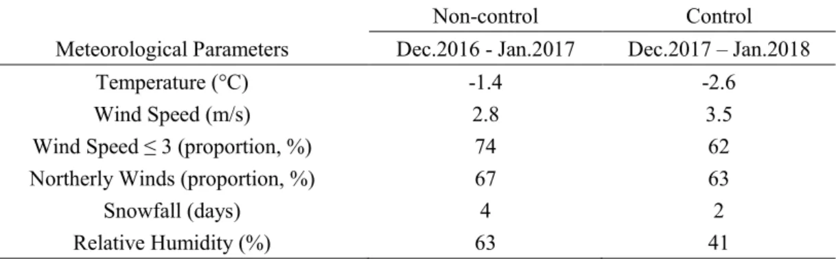
Line 258-264: In addition, we discussed several meteorological parameters in Beijing during the
study period (Table S4). Temperature, wind speed and wind direction data were acquired from National
Oceanic and Atmospheric Administration (https://www.noaa.gov/), snowfall and relative humidity data
were from China Meteorological Administration (http://www.cma.gov.cn/). Little snowfall, low speed (
≤3 m/s)
winds and northerly winds were dominant during both the non-control and control periods, and the
differences of average temperature and average wind speed between the two periods were 1.2
°Cand 0.7
m/s, respectively, indicating the minor influence from meteorological variability on the change of VOC
mixing ratios.
3
Table S4. Summary of average meteorological parameters during the non-control and control periods.
Meteorological Parameters
Non-control Control Dec.2016 - Jan.2017 Dec.2017 – Jan.2018
Temperature (°C) -1.4 -2.6
Wind Speed (m/s) 2.8 3.5
Wind Speed ≤ 3 (proportion, %) 74 62
Northerly Winds (proportion, %) 67 63
Snowfall (days) 4 2
Relative Humidity (%) 63 41
a Meteorological data were all measured at a time interval of 0.5 h. b Northerly wind includes NW, NNW, N, NNE, NE.
2. The authors report “total VOC”, when referring to sum measured VOC. When this term is first used
some discussion of the limitations of the measurement technique and which VOC species may not be
included here is required (e.g. methanol and ethanol).
Response: Accepted.
We apologize for the unclarity in the manuscript. We have added some discussions
about the limitations of the measurement technique and pointed VOC species not included in the study,
see section 2.2. The details are given as follows:
Line 93-102: Calibration curves were performed at six mixing ratios from 0.2 to 8 ppbv for each
compound before and after sample analyses by bubbling a series of external calibrating gases. Two types
of gases were used: a Photochemical Assessment Monitoring Stations (PAMS) ozone precursor series
(mixture of 57 NMHCs), and a gas series customized by the PKU National Key Laboratory (a mixture of
55 oxygenated VOCs and halocarbons). In addition, internal calibrating gases were pumped into the
GC-MS system
once sampling or calibrating to reduce instrumental error. All four calibrating gases were
obtained from Linde Electronics and Specialty Gases, USA. R2 (coefficient of determination) values of
eligible calibration curves are > 0.99. VOC species can be quantified only if they have eligible calibration
curves. Several VOC species also cannot be quantified because their mixing ratios were below method
detection limit (MDL). Finally, a total of 91 VOC species were quantified (Table S5), not including
formaldehyde, acetaldehyde, and alcohols.
3. “Mixing ratio” and “concentration” are used interchangeably throughout (e.g. lines 226 and 229).
Where referring to values in ppb “mixing ratio” should be used.
Response: Accepted.
Thanks for pointing out the error and we have checked through the manuscript
carefully to ensure the reasonable using of “mixing ratio” and “concentration”.
4
4. Line 2: Define “heating season” in the abstract.
Response: Accepted.
The definition of heating season was adjusted in the introduction, and added in the
abstract. The definition is “the cold season when fossil fuel is burned for residential heating”.
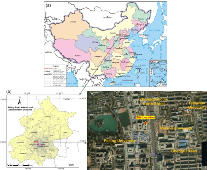
5. Line 85: Figure S1 does not do much to allow the reader to learn more about the site location. I suggest
zooming in further on the right hand image and adding details to the map.
Response: Accepted.
According to your justified comment, we have redrawn Figure S1 as below.
Sources of base maps were given in the caption.
Figure S1. The location of (a) Beijing in China (http://bzdt.ch.mnr.gov.cn/) and (b) Peking University (PKU) in Beijing (http://openstreetmap.org/); and (c) the surroundings of the sampling site at PKU (https://www.mapbox.com/).
5
6. Line 91: Describe the “rigorous” QA and QC procedures applied.
Response: Accepted.
Thank you for pointing out our omission. We have explained the “rigorous” QA
and QC procedures in section 2.2 as shown below:
Line 103-108: We applied rigorous quality-assurance (QA) and quality-control (QC) procedures
which included three main parts. First, daily maintenance and monitoring of the online GC–MS/FID
system were performed to ensure the normal operation of instrument. Second, periodic supplement and
replacement of consumable items were performed at least every 10 days to ensure the operation of
automatic sampling and measuring. Third, periodic calibrations were performed every 5 days, and the
calibration curve results of each target species with <
10% variation were considered acceptable relative
to the actual values.
7. Line 102: What was the signal to noise threshold for the compounds not included and why was this
value chosen? Line 106: By what criteria were VOCs categorised as “bad”?
Response: Accepted.
In the revised version of our manuscript, we added the signal to noise threshold for
VOC species omitted form PMF analysis and criteria for species defined as “bad”, and we gave some
explanation about them in section 2.3.
Line 118-120: According to the input files, signal-to-noise ratio (S:N) was calculated for each species,
and only mixing ratios that exceed the uncertainty contribute to the signal portion in the PMF version we
used. Signal is the difference between mixing ratio and uncertainty and noise is the uncertainty value.
Line 122-127: A species is not appropriate for source apportionment if it is undetectable (< MDL) in
most of the samples or its mixing ratio always below the uncertainty (signal = 0). Therefore, VOC species
that were below the MDL in >
50% of samples or that showed S:N
= 0 were categorized as “bad” directly.
Other species were categorized based on detailed knowledge of the sources, sampling, and analytical
uncertainties (Reff et al., 2007). For species without detailed information, as mentioned in PMF user
guide, we conservatively categorized them as “good” if S:N > 1, “Bad” if S:N < 0.5 and “Weak” if S/N <
1 but > 0.5.
8. Line 113: Systematic literature reviews generally follow a clearly defined protocol. I suggest defining
the criteria used in the review or deleting “systematic”.
Response: Accepted.
Thank you for pointing out our inappropriate expression. We browsed most of the
literature about anthropogenic VOC emission inventory but the procedure is subjective and cannot be
described explicitly, therefore, we deleted “systematic” as you suggested. (Line 134)
9. Line 129: When stating “Many studies” please provide citations.
Response: Accepted.
We have provided the citations when stating “many studies” as below:
6
et al., 2017;Huo et al., 2017;Peng et al., 2019), but few of that have estimated SC reductions in 2017
compared to 2016.
10. Line 202: Add citation for the reduction of civil SC in Beijing exceeding 2 million tons or describe
where this figure is from? Figs 1 and 2: Where are these data from?
Response: Accepted.
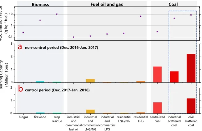
Thank you for pointing out our omission. Fig 1 and Line 202: for fuel consumption,
all relevant data were directly given in or deduced from China Energy Statistical Yearbook (CESY) and
COALCAP report; for emission factors, exact values and their detailed references were provided in Table
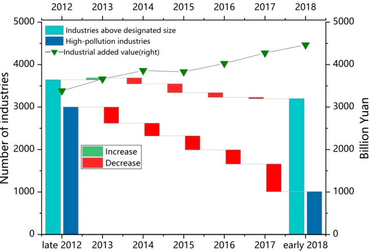
S1. Fig 2: industrial added value and quantity of industries above designated size were from Beijing
Municipal Bureau Statistics (BBS, http://tjj.beijing.gov.cn/); quantity of high-pollution industries was
from Beijing Municipal Ecology and Environment Bureau (BMEE,
http://sthjj.beijing.gov.cn/
). We have
added these citations as you suggested as below:
Line 227-228: Compared to 2016, the reduction of civil SC consumption in Beijing exceeded 2
million tons in 2017 (CESY, 2017 – 2018; COALCAP reports, 2017 – 2018).
Line 234-238: As shown in Fig. 1, compared with other fuel types, SC is consumed more in winter
(CESY, 2017 – 2018; COALCAP reports, 2017 – 2018), and has greater VOC emissions per unit
combustion (see Table S1 for details).
Line 247-249: The annual variations of industries above designated size (BBS), high-pollution
industries (BMEE), and the annual benefits from industry (BBS) in Beijing are summarized in Fig. 2.
11. Line 214: Define “designed size enterprise”
Response: Accepted.
To make it clear, we referred the expression given in the statistical yearbook and
fixed “designed size enterprise” as “industry above designated size”. Industry above designated size is
defined as industry with an annual main business income of more than 20 million yuan. (Line 249-250)
12. Fig 2: Does the industrial added value refer to just the designed size enterprises and high pollution
enterprises or is this a Beijing total?
Response: Accepted.
The industrial added value provided here is a Beijing total, which is the sum of
added value of all industrial units in Beijing. (Line 250)
13. Section 3.2. A discussion of the VOC mixing ratios recorded in this study at the start of this section
would
provide context for the % reductions reported. Without knowing how
high mixing ratios were it’s
hard for the reader to interpret the % reductions. This could
be achieved by adding mixing ratios to table
1.
Response: Accepted.
Thank you for underlining this deficiency. The modified Table 1 has replaced the
old version in the manuscript, and we gave it as below:
7
Table 1. The 20 VOC species which declined the most following emissions controls during strict-control and eased-control periods. Species non-control (ppbv) strict-control (ppbv) Decreasing ratio (%) Species non-control (ppbv) eased-control (ppbv) Decreasing ratio (%) methacrolein 1.18 0.25 78.8% cyclohexane 0.11 0.03 72.7%
methyl ethyl ketone 0.78 0.22 71.8% 1,2-dichloropropane 0.51 0.14 72.5%
benzene 3.27 1.06 67.6% acrolein 0.14 0.04 71.4%
styrene 0.37 0.12 67.6% 1,1-dichloroethane 0.17 0.05 70.6%
1,2-dichloropropane 0.51 0.18 64.7% styrene 0.37 0.11 70.3%
acrolein 0.14 0.05 64.3% methyl vinyl ketone 0.50 0.15 70.0%
methyl vinyl ketone 0.50 0.18 64.0% benzene 3.27 1.03 68.5%
acetylene 8.98 3.40 62.1% m/p-xylene 0.85 0.28 67.1% ethylene 12.07 4.60 61.9% cis-2-butene 0.09 0.03 66.7% m/p-xylene 0.85 0.33 61.2% isoprene 0.12 0.04 66.7% propanal 0.53 0.21 60.4% ethylene 12.07 4.03 66.6% 1,4-dichlorobenzene 0.20 0.08 60.0% toluene 3.63 1.26 65.3% toluene 3.63 1.47 59.5% o-xylene 0.65 0.23 64.6% 1,1-dichloroethane 0.17 0.07 58.8% propylene 2.10 0.75 64.3% isoprene 0.12 0.05 58.3% acetylene 8.98 3.21 64.3% o-xylene 0.65 0.28 56.9% propanal 0.53 0.19 64.2%
acetone 6.37 2.77 56.5% methyl ethyl ketone 0.78 0.28 64.1%
ethylbenzene 0.96 0.42 56.3% ethylbenzene 0.96 0.35 63.5%
propylene 2.10 0.92 56.2% 3-methyl pentane 0.61 0.23 62.3%
cis-2-butene 0.09 0.04 55.6% acetone 6.37 2.46 61.4%
14. Fig 3. See earlier comment, which VOCs are included in this figure? If reporting ppb suggest changing
the “concentration” to “mixing ratio” in the caption
Response: Accepted.
Thank you for your suggestion. We have changed the “concentration” to “mixing
ratio” in Fig. 3, as shown below.
8
Figure 3. Ambient VOC mixing ratios (ppbv) in different seasons of Beijing.
15. Fig 4: Add names and citations for previous studies shown.
Response: Accepted.
Thank you for pointing out our omission. Names and citations have been added in
Fig. 4 to clarify their sources as shown below.
Figure 4. The ratios of benzene and toluene in different seasons (previous studies) and different control periods (this study).
9
Minor comments:
1. Line 62: Suggesting changing “400×104” to “4×10⁶”
Response: Accepted.
We have made change as you suggested. (Line 62)
2. Figure S4: Label figure to show control and non-control periods (i.e. which is top and which is bottom).
Response: Accepted.
We have added labels in Figure S4 to give a clear indication.
Figure S4: Full-time variations in mixing ratios of eight sources in Beijing during the (a) non-control and (b) control periods.
3. Lines 204 – 207: This sentence isn’t very clear, suggest rewording
Response: Accepted.
This sentence has been reworded. The details are given as follows:
Line 234-238:
A large proportion of civil SC (> 90%) is used for heating in winter. As shown in Fig.
1, compared with other fuel types, SC is consumed more in winter (CESY, 2017 – 2018; COALCAP
Reports, 2017 – 2018), and has greater VOC emissions per unit combustion (see Table S1 for details). As
for industrial SC burning, sustained clampdown of the coal-fired boilers was put into action in Beijing
from 2013, and
99.8%
of them had been banned before late 2017. These banned boilers contributed nearly
9 million tons of SC reductions and more than half of them were eradicated in 2017.
10
4. Line 212: Suggest changing “part” to “number”
Response: Accepted.
We have made change as you suggested. (Line 245)
5. Line 251: “top 20 most decreased VOC species” is a slightly confusing term. This term is used
throughout this section. I suggest changing to “the 20 VOC species which declined the most following
emissions controls”.
Response: Accepted.
We have modified this expression throughout the section according to the comment.
6. Line 252: Suggest adding “mixing ratios of the” after “period,”
11
References:
Jia Y.T., Rahn K.A., He K.B., Wen T.X., and Wang Y.S.: A novel technique for quantifying the regional component of urban aerosol solely from its sawtooth cycles, Journal of Geophysical Research-Atmospheres, 113, D21309, 2008.
Cheng, M. M., Zhi, G. R., Tang, W., Liu, S. J., Dang, H. Y., Guo, Z., Du, J. H., Du, X. H., Zhang, W. Q., Zhang, Y. J., and Meng, F.: Air pollutant emission from the underestimated households coal consumption source in China, Sci. Total Environ., 580, 641-650, 10.1016/j.scitotenv.2016.12.143, 2017.
Huo, M. L., Zhao, J., Xu, Z., Shan, B. G., and Jia, D. X.: China Scattered Coal Consumption Map and Influence Factors, Electric Power, 50, 1-8, 10.11930/j.issn.1004-9649.201701147, 2017.
Liu, H. B., Kong, S. F., Wang, W., and Yan, Q.: Emission inventory of heavy metals in fine particles emitted from residential coal burning in China, 37, 2823-2835, 10.13227/j.hjkx.2016.08.002, 2016.
Peng, L. Q., Zhang, Q., Yao, Z. L., Mauzerall, D. L., Kang, S. C., Du, Z. Y., Zheng, Y. X., Xue, T., and He, K. B.: Underreported coal in statistics: A survey-based solid fuel consumption and emission inventory for the rural residential sector in China, Applied Energy, 235, 1169-1182, 10.1016/j.apenergy.2018.11.043, 2019.
Reff, A., Eberly, S. I., and Bhave, P. V.: Receptor modeling of ambient particulate matter data using positive matrix factorization: Review of existing methods, J. Air Waste Manage., 57, 146-154, 10.1080/10473289.2007.10465319, 2007.
Li, J., Xie, S. D., Zeng, L. M., Li, L. Y., Li, Y. Q., and Wu, R. R.: Characterization of ambient volatile organic compounds and their sources in Beijing, before, during, and after Asia-Pacific Economic Cooperation China 2014, Atmos. Chem. Phys., 15, 7945-7959, 10.5194/acp-15-7945-2015, 2015a.
Li, L. Y., Xie, S. D., Zeng, L. M., Wu, R. R., and Li, J.: Characteristics of volatile organic compounds and their role in ground-level ozone formation in the Beijing-Tianjin-Hebei region, China, Atmos. Environ., 113, 247-254, 10.1016/j.atmosenv.2015.05.021, 2015b.
Li, J., Wu, R. R., Li, Y. Q., Hao, Y. F., Xie, S. D., and Zeng, L. M.: Effects of rigorous emission controls on reducing ambient volatile organic compounds in Beijing, China, Sci. Total Environ., 557, 531-541, 10.1016/j.scitotenv.2016.03.140, 2016c. Li, J., Hao, Y. F., Simayi, M., Shi, Y. Q., Xi, Z. Y., and Xie, S. D.: Verification of anthropogenic VOC emission inventory
through ambient measurements and satellite retrievals, Atmos. Chem. Phys., 19, 5905-5921, 10.5194/acp-2018-1133-ac1 2019b.
12
Anonymous Referee #2:
General Comments:
The authors have addressed all my comments; I suggest accepting it.
Response:
Thank you for your letter dated 24 May, 2020. We were pleased to know that our work was
suggested as acceptable for publication in
Atmospheric Chemistry and Physics
after addressing your
comments. We thank you again for your constructive criticisms that have helped us to improve our
manuscript.
13
Responds to the editor’s comments:
Comments to the Author:
I am happy that the authors have addressed all of the comments made by the reviewers and am suggesting
that the manuscript is published once the following few corrections are made:
Technical Corrections:
1. Line 90 – 93: ‘calibrating gases was pumped into..’ to ‘calibrating gases were pumped into..’
Response: Accepted.
Revised version: In addition, internal calibrating gases were pumped into the GC-MS system once
sampling or calibrating to reduce instrumental error.
2. ‘We applied rigorous quality-assurance (QA) and quality-control (QC) procedures which including
three main parts’ to ‘We applied rigorous quality-assurance (QA) and quality-control (QC) procedures
which included three main parts’
Response: Accepted.
Revised version: We applied rigorous quality-assurance (QA) and quality-control (QC) procedures
which including three main parts.
3 Line 116 – 118: ‘A species is not proper for source apportionment if it is undetectable (< MDL) in most
of samples’ to ‘A species is not appropriate for source apportionment if it is undetectable (< MDL) in
most of the samples’
Response: Accepted.
Revised version: A species is not appropriate for source apportionment if it is undetectable (< MDL)
in most of the samples or its mixing ratio always below the uncertainty (signal = 0).
4. Line 165: ‘Most of monthly data..’ to ‘Most of the monthly data..’
Response: Accepted.
Revised version: Most of the monthly data
for industrial sector emissions were developed based on
outputs of industrial products issued by National Bureau of Statistics of China (NBS,
http://www.stats.gov.cn/) and Beijing Municipal Bureau Statistics (BBS, http://tjj.beijing.gov.cn/).
5. Line 229 – 234: ‘emerged’ to eradicated’
Response: Accepted.
Revised version: These banned boilers contributed nearly 9 million tons of SC reductions and more
than half of them were eradicated in 2017.
14
6. Line 246 – 247: ‘with annual main business income..’ to ‘with an annual main business income..’
Response: Accepted.
Revised version: Industry above designated size is defined as industry with an annual main business
income of more than 20 million yuan.
1
List of all relevant changes made in the manuscript
Position in the
revised version
Previous version
Revised version
Line 9
(the cold season when fossil fuel is burned for residential heating)
Line 12/ 34/ 68/
112/ 266/ 268/ 438/
444/ 445/ 446
concentrations
mixing ratios
Line 16/ 318
analyses
analysis
Line 35
when centralized district heating is turned on the cold season when fossil fuel is burned for residential heating
Line 62
at 400×10
4t
at 4 × 10
6t
Line 71/ 130/ 813/
820
concentration
mixing ratios
Line 90-93
We applied rigorous quality-assurance (QA)
and quality-control (QC) procedures. Daily
calibrations were performed every 5 days, and
the calibration curve results of each target
species with <10% variation were considered
acceptable relative to the actual
concentrations. Detailed information is shown
in Text S1.
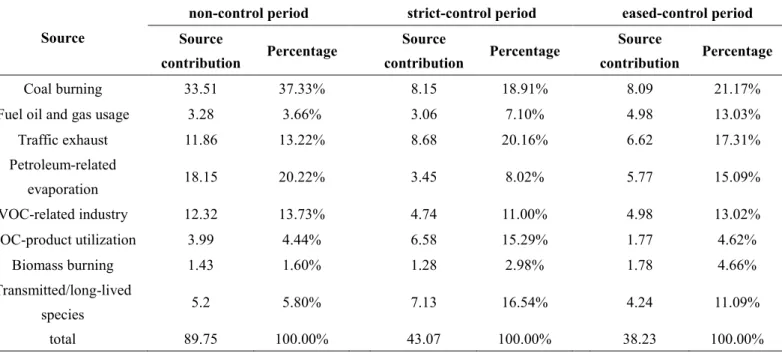
Detail of the online system is shown in Text S1. Calibration curves were performed at six mixing
ratios from 0.2 to 8 ppbv for each compound before and after sample analyses by bubbling a series
of external calibrating gases. Two types of gases were used: a Photochemical Assessment
Monitoring Stations (PAMS) ozone precursor series (mixture of 57 NMHCs), and a gas series
customized by the PKU National Key Laboratory (a mixture of 55 oxygenated VOCs and
halocarbons). In addition, internal calibrating gases were pumped into the GC-MS system once
sampling or calibrating to reduce instrumental error. All four calibrating gases were obtained from
Linde Electronics and Specialty Gases, USA. R2 (coefficient of determination) values of eligible
calibration curves are > 0.99. VOC species can be quantified only if they have eligible calibration
curves. Several VOC species also cannot be quantified because their mixing ratios were all below
method detection limit (MDL). Finally, a total of 91 VOC species were quantified (Table S5), not
including formaldehyde, acetaldehyde, and alcohols.
The MDL for each species quantified using
this system ranged from 0.01 to 0.10 ppbv. We applied rigorous quality-assurance (QA) and
quality-control (QC) procedures which included three main parts. First, daily maintenance and
monitoring of the online GC–MS/FID system were performed to ensure the normal operation of
instrument. Second, periodic supplement and replacement of consumable items were performed at
least every 10 days to ensure the operation of automatic sampling and measuring. Third, periodic
calibrations were performed every 5 days, and the calibration curve results of each target species
2
with < 10% variation were considered acceptable relative to the actual values.
Line 114/ 291
concentration
mixing ratio
Line 116-118
VOC species that were below the MDL
in >50% of samples or that showed a very
small signal-to-noise ratio (S:N) were omitted
from analyses. S:N was calculated for each
species using PMF, where the signal
represents the difference between
concentration and uncertainty.
According to the input files, signal-to-noise ratio (S:N) was calculated for each species, and only
mixing ratios that exceed the uncertainty contribute to the signal portion in the PMF version we
used. Signal is the difference between mixing ratio and uncertainty and noise is the uncertainty
value.
We categorized VOC species as “strong,” “weak,” and “bad.” Strong was the default value for all
species, weak indicates those with tripled uncertainty, and VOCs categorized as bad were removed
from further analyses. A species is not appropriate for source apportionment if it is undetectable
(< MDL) in most of the samples or its mixing ratio always below the uncertainty (signal = 0).
Therefore, VOC species that were below the MDL in > 50% of samples or that showed S:N = 0
were categorized as “bad” directly. Other species were categorized based on detailed knowledge
of the sources, sampling, and analytical uncertainties (Reff et al., 2007). For species without
detailed information, as mentioned in PMF user guide, we conservatively categorized them as
“good” if S:N > 1, “Bad” if S:N < 0.5 and “Weak” if S:N < 1 but > 0.5.
Line 134
systematic
delete
Line 148-149
For other emission sources, we relied on EFs
and source profiles provided in the
pre-established emission inventory for the
Beijing–Tianjin–Hebei (BTH) region
For EFs and source profiles of other emission sources, we relied on multiple technical manuals
about VOC emissions estimation, which are mostly issued by Ministry of Ecology and
Environment of the People’s Republic of China (MEE, http://www.mee.gov.cn/), and the
pre-established emission inventory for the Beijing–Tianjin–Hebei (BTH) region
Line 153
Many studies have estimated the SC
consumption recent years
Many studies have estimated the SC consumption recent years (Liu et al., 2016a;Cheng et al.,
2017;Huo et al., 2017;Peng et al., 2019)
Line 165
Most of monthly data for industrial sector
emissions were developed based on outputs of
industrial products (NBS/BBS).
Most of the monthly data for industrial sector emissions were developed based on outputs of
industrial products issued by National Bureau of Statistics of China (NBS,
http://www.stats.gov.cn/) and Beijing Municipal Bureau Statistics (BBS, http://tjj.beijing.gov.cn/).
Line 228
(CESY, 2017 – 2018; COALCAP reports, 2017 – 2018)
Line 229-234
SC is consumed more, and has greater VOC
emissions per unit combustion, than other fuel
types (Fig. 1). Also, a large proportion of civil
SC (> 90%) is used for heating in winter. As
for industrial sector, sustained clampdown of
A large proportion of civil SC (> 90%) is used for heating in winter. As shown in Fig. 1, compared
with other fuel types, SC is consumed more in winter (CESY, 2017 – 2018; COALCAP reports,
2017 – 2018), and has greater VOC emissions per unit combustion (see Table S1 for details). As
for industrial SC burning, sustained clampdown of the coal-fired boilers was put into action in
Beijing from 2013, and 99.8% of them had been banned before late 2017. These banned boilers
3
the coal-fired boilers was put into action in
Beijing from 2013, 99.8% of the boilers
associated with nearly 9 million tons of SC
consumption annually were banned and more
than half of that were emerged in 2017. All the
industrial scattered coal was eradicated by the
end of 2017.
contributed nearly 9 million tons of SC reductions and more than half of them were eradicated in
2017.
Line 243-244
Meanwhile, a large part of high-pollution
enterprises (those heavy polluting industries
as stipulated by the state environmental
protection department)
Meanwhile, a large number of high-pollution industries, which are stipulated by Beijing Municipal
Ecology and Environment Bureau (BMEE, http://sthjj.beijing.gov.cn/)
Line 246-247
The annual variation of designed size
enterprises, high-pollution enterprises, and the
annual benefits from industry in Beijing are
summarized in Fig. 2.
The annual variations of industries above designated size (BBS), high-pollution industries
(BMEE), and the annual benefits from industry (BBS) in Beijing are summarized in Fig. 2.
Industry above designated size is defined as industry with an annual main business income of more
than 20 million yuan. Industrial added value refers to the sum of added value of all industrial units
in Beijing.
Line 258-264
In addition, we discussed several meteorological parameters in Beijing during the study period
(Table S4). Temperature, wind speed and wind direction data were acquired from National Oceanic
and Atmospheric Administration (https://www.noaa.gov/), snowfall and relative humidity data
were from China Meteorological Administration (http://www.cma.gov.cn/). Little snowfall, low
speed
(≤ 3
m/s) winds and northerly winds were dominant during both the non-control and control
periods, and the differences of average temperature and average wind speed between the two
periods were 1.2 °C and 0.7 m/s, respectively, indicating the minor influence from meteorological
variability on the change of VOC mixing ratios.
Line 290
concentrations
mixing ratio
Line 292
concentration
contribution
Line 293
The top 20 most-decreased VOC species after
control measures
The 20 VOC species which declined the most following emissions controls
Line 284
mixing ratios of the
Line 302
concentrations
contributions
4
Line 811
The top 20 major VOC species with the
highest decreasing ratios compared with
non-control period.
The 20 VOC species which declined the most following emissions controls during strict-control
and eased-control periods.
Line 817-818
Quantities and variations of designed size
enterprises and high-pollution enterprises
from late 2012 to early 2018 (bridge figure),
and industrial added value from 2012 to 2018
(line).
Quantities and variations of industries above designated size and high-pollution industries from
late 2012 to early 2018 (bridge figure), and industrial added value from 2012 to 2018 (line).
Line 832
Modify Table 1.
Supplementary
Information
Figure S1. The location of Beijing in China
(red area) and the sampling site at Peking
University, Beijing (red point).
Figure S1. The location of (a) Beijing in China (http://bzdt.ch.mnr.gov.cn/) and (b) Peking
University (PKU) in Beijing (http://openstreetmap.org/); and (c) the surroundings of the sampling
site at PKU (https://www.mapbox.com/).
Supplementary
1
Scattered coal is the largest source of ambient volatile organic
compounds during the heating season in Beijing
Yuqi Shi
1, Ziyan Xi
1, Maimaiti Simayi
1, Jing Li
1,2, Shaodong Xie
11College of Environmental Sciences and Engineering, State Key Joint Laboratory of Environmental Simulation and Pollution Control, Peking University, Beijing, 100871, PR China
5
2Department of Environmental Health, Harvard T.H. Chan School of Public Health, Boston, 02215, USA
Correspondence to:Shaodong Xie([email protected])
Abstract. We identified scattered coal burning as the largest contributor to ambient volatile organic compounds (VOCs), exceeding traffic-related emissions, during the heating season (the cold season when fossil fuel is burned for residential heating)
in Beijing prior to the rigorous emission limitations enacted in 2017. However, scattered coal is underestimated in emission 10
inventories generally, because the activity data are incompletely recorded in official energy statistics. Results of positive matrix factorization (PMF) models confirmed that coal burning was the largest contributor to VOC mixing ratios concentrations prior to the emission limitations of 2017, and a reduction in scattered coal combustion, especially in rural residential sector, was the primary factor in the observed decrease in ambient VOCs and secondary organic aerosol (SOA) formation potential in urban Beijing after 2017. Scattered coal burning was included in a corrected emission inventory and we obtained comparable results 15
between this corrected inventory and PMF analysis analyses, particularly for the non-control period. However, a refined source sub-classification showed that passenger car exhaust, petrochemical manufacturing, gas stations, traffic evaporation, traffic equipment manufacturing, painting, and electronics manufacturing are also contributors to ambient VOCs. These sources should focus on future emission reduction strategies and targets in Beijing. Moreover, in other region with scattered coal-based heating, scattered coal burning is still the key factor to improve the air quality in winter.
2 1Introduction
In Chinese cities, a severe deterioration in air quality has threatened human health (Han et al., 2018). Extremely poor air quality in cities such as Beijing, one of the world’s largest and China’s capital, is a result of growth in fossil-fuel economies, the expansion of industrial manufacturing, heavy traffic, and large-scale urban construction (Ru et al., 2015;Zeng et al., 2005;Liu and Wu, 2013;Tang, 2007). Within China, organizations such as the Joint Prevention and Control of Atmospheric Pollution 25
(JPCAP) and Regional Atmospheric Pollution Control (RAPC) have identified volatile organic compounds (VOCs) as key air pollutants (Zhou and Elder, 2013). VOCs are precursors of secondary organic aerosols (SOAs), which are in turn related to
particulate matter < 2.5 μg (PM2.5), and photochemically produced ozone (O3) (Sillman, 1999;Pandis, 1997). The negative effects of VOCs on human health have received increased public attention (Logue et al., 2010;Zhang et al., 2012). Globally, natural sources are significant emitters of VOCs, however, anthropogenic sources are far more prevalent in urban areas 30
(Guenther et al., 2006;Janssens-Maenhout et al., 2015), particularly in winter at northern latitudes when biological emissions are low (Li and Xie, 2014). Therefore, it is important to incorporate seasonality into understanding major anthropogenic sources of VOCs and in developing effective controls and mitigation measures for air pollution.
Ambient VOC mixing ratios concentrations in Beijing show significant seasonal variation and are highest during the heating season (November to March, the cold season when fossil fuel is burned for residential heating when centralized district heating 35
is turned on) (Liu et al., 2005;Wang et al., 2014;Wei et al., 2018). Satellite-derived emission inventories have suggested monthly variation in total VOC emissions, with distinct highs during the heating season (Li et al., 2019b). Results of source apportionment analyses have indicated differences in source contributions of VOCs seasonally, with high proportions coming from coal combustion during the heating season and traffic exhaust in the remaining months (Wang et al., 2014;Wang et al., 2013a). However, most emission factor (EF)-based inventories do not include seasonal variation.
40
Scattered coal (SC) is defined as those coal of poor quality which is dispersedly used in civilian (households cooking and heating, commercial and public, rural production, etc.), and industry (small-scale industrial boilers and furnaces). The coal of poor quality, with high content of ash, sulfur and volatile matters, is widely used in rural residential sector due to the low price,
3
besides, it is different to cover those decentralize-used coal overall in official energy statistics (Cheng et al., 2017;Peng et al., 2019;Huo et al., 2017). Different from efficient centralized coal combustion, such as power generation, heat supply and large-45
scale industrial boilers, SC burning is a near-ground and non-point source, its low combustion efficiency and air pollution control deficiency results in higher air pollutant emission intensity, which brings negative influence on ambient air and has a more direct adverse impact on the human health (Finkelman et al., 1999).
Especially, as a major ambient pollution source, household energy consumption has attributed a large number of deaths especially in rural areas (Zhao et al., 2019), and attracts more and more public attention (Liu et al., 2016b). It's undeniable that 50
a reduction in conventional household solid fuel consumption has improved air quality and human health in northern China over recent decades (Zhao et al., 2018). Nevertheless, solid fuel combustion remains an important emission source. Moreover, rural residential coal combustion affects not only rural but urban air quality, and has higher contributions in winter especially in northern China for a long time (Shen et al., 2019). However, a large proportion of residential coal use is overlooked in China Energy Statistical Yearbook (CESY), which means that most EF-based inventories may poorly estimate coal consumption. 55
Using field sampling and remote sensing, many studies have showed that the actual amount of rural and urban coal consumption is much higher than the statistical data in CESY. Peng et al. (2019) conducted a field survey in 2010 to obtain data for solid fuel consumption and use patterns in Chinese counties, and accordingly estimated 62% higher than the coal consumption reported in CESY for the rural residential sector in China. Cheng et al. (2017) summarized the investigated coal consumption of several studies in rural area, and estimated the residential coal consumption from 1996 to 2014 in the BTH 60
region, which triples coal consumption reported in CESY. Cheng et al. (2016) also estimated Beijing’s residential coal combustion at 4 × 10⁶ t at 400×104 t in 2015. Previous research, combined with the prevalence of coal-based heating in northern China (Wang et al., 2013a), suggests that coal combustion is an important contributor to ambient VOCs over winter, but the magnitude of this contribution is not yet understood. Li et al. (2019b) showed similar PMF results in an evaluation of emissions in the winter of 2015 in Beijing, where fuel combustion contributed > 50% of ambient VOCs. They also proposed that the 65
4
essential parts of fuel combustion might be the undocumented consumption of coal briquettes and chunks, but did not give any further explicit evidence.
We focused on confirming SC burning as a critical anthropogenic VOC emission source contributing to high VOC mixing ratios concentrations during the heating season in Beijing. We discuss the efficacy of air pollution control periods in light of observed variation in emission intensities. We used the positive matrix factorization (PMF) model to quantify the contributions 70
of different emission sources to observed VOC mixing ratios concentration data. The contribution of coal burning was confirmed by examining variation among emission sources, control measures placed on sources, and emission intensities. We estimated a monthly corrected EF-based inventory for the heating season, and compared these estimates to the PMF results. We calculated secondary organic aerosols potential (SOAP) values for different emission sources based on the results of the PMF and emission inventory to determine the largest contributor to total SOAP reduction. We further evaluate and discuss the 75
control policies of 2017.
2 Methods
2.1 Site description
Air quality measurements were collected during two consecutive heating seasons, the first from December 2016 to January 2017, when air quality control measures were not heavily enforced (non-control period), and the second from December 2017 80
to January 2018, when air quality control measures were rigorously enforced (control period). Measurements were taken at the fifth story of a building on the Peking University (PKU) campus in northwestern Beijing (39.99°N, 116.33°E), at a height of approximately 12 m. The building was surrounded by several five- or six-story buildings and one side road to the east. This site is located approximately 700 m north of 4th ring road (a major city traffic line) and 10 km from the centre of Beijing (Fig. S1). The surrounding area is primarily commercial and residential, and the major nearby emission source is road vehicles. This 85
5 2.2 Sampling and analyses
We used a continuous sampling and analyses method for ambient VOCs, which has been described in detail in previous studies (Wu et al., 2016b;Li et al., 2015a). Automated, hourly sample collection was achieved using a custom-built online GC–MS/FID system (TH-PKU 300B, Wuhan Tianhong Instrument Co. Ltd., China; GCMS-QP2010SE, Shimadzu, Japan). We applied 90
rigorous quality-assurance (QA) and quality-control (QC) procedures. Daily calibrations were performed every 5 days, and the calibration curve results of each target species with <10% variation were considered acceptable relative to the actual concentrations. Detailed information is shown in Text S1. Detail of the online system is shown in Text S1. Calibration curves were performed at six mixing ratios from 0.2 to 8 ppbv for each compound before and after sample analyses by bubbling a series of external calibrating gases. Two types of gases were used: a Photochemical Assessment Monitoring Stations (PAMS)
95
ozone precursor series (mixture of 57 NMHCs), and a gas series customized by the PKU National Key Laboratory (a mixture of 55 oxygenated VOCs and halocarbons). In addition, internal calibrating gases were pumped into the GC-MS system once sampling or calibrating to reduce instrumental error. All four calibrating gases were obtained from Linde Electronics and Specialty Gases, USA. R2 (coefficient of determination) values of eligible calibration curves are > 0.99. VOC species can be quantified only if they have eligible calibration curves. Several VOC species also cannot be quantified because their mixing
100
ratios were all below method detection limit (MDL). Finally, a total of 91 VOC species were quantified (Table S5), not including formaldehyde, acetaldehyde, and alcohols. The MDL for each species quantified using this system ranged from 0.01 to 0.10 ppbv. We applied rigorous quality-assurance (QA) and quality-control (QC) procedures which included three main parts. First, daily maintenance and monitoring of the online GC–MS/FID system were performed to ensure the normal operation of instrument. Second, periodic supplement and replacement of consumable items were performed at least every 10
105
days to ensure the operation of automatic sampling and measuring. Third, periodic calibrations were performed every 5 days, and the calibration curve results of each target species with < 10% variation were considered acceptable relative to the actual values.
6 2.3 Source apportionment
The USEPA PMF model (version 5.0) has been applied to a wide range of data, including 24 h speciated PM2.5, size-resolved 110
aerosols, deposition, air toxins, high-time-resolution measurements such as those from aerosol mass spectrometers (AMSs), and VOC mixing ratios concentrations. As a receptor model, PMF is a mathematical approach. Composition or speciation is determined using analytical methods appropriate for the media. We applied this PMF model to determine source apportionment for measured ambient VOCs. A PMF requires two input files: a mixing ratio concentration dataset comprising a suite of parameters measured across multiple samples, and an uncertainty dataset comprising uncertainty values for each species and 115
sample. VOC species that were below the MDL in >50% of samples or that showed a very small signal-to-noise ratio (S:N) were omitted from analyses. S:N was calculated for each species using PMF, where the signal represents the difference between concentration and uncertainty. According to the input files, signal-to-noise ratio (S:N) was calculated for each species, and only mixing ratios that exceed the uncertainty contribute to the signal portion in the PMF version we used. Signal is the difference between mixing ratio and uncertainty and noise is the uncertainty value.
120
We categorized VOC species as “strong,” “weak,” and “bad.” Strong was the default value for all species, weak indicates those with tripled uncertainty, and VOCs categorized as bad were removed from further analyses. A species is not appropriate for source apportionment if it is undetectable (< MDL) in most of the samples or its mixing ratio always below the uncertainty (signal = 0). Therefore, VOC species that were below the MDL in > 50% of samples or that showed S:N = 0 were categorized as “bad” directly. Other species were categorized based on detailed knowledge of the sources, sampling, and analytical
125
uncertainties (Reff et al., 2007). For species without detailed information, as mentioned in PMF user guide, we conservatively categorized them as “good” if S:N > 1, “Bad” if S:N < 0.5 and “Weak” if S:N < 1 but > 0.5. The final dataset comprised 1,918 samples of 53 compounds (42 strong and 11 weak), which accounted for 90% of the total mixing ratios. Modeling was performed using 4 – 11 factors and the 8-factor solution was deemed to be the most representative. In profile analysis technology, ambient VOC mixing ratios concentration can be considered the linear addition of VOC compositions derived 130
7
from various sources. Characteristics of each pollution source can be used, to some extent, to resolve issues with collinearity in the source component spectrum.
2.4 VOC emission inventory
Through systematic literature review we found that while anthropogenic VOC emission inventory methodologies are similar, source classification and EFs differ between studies. To promote the comparability of PMF and emission inventory results we 135
proposed and utilized a modified source classification system based on the existing four-level categorization (Wu et al., 2016a). Level 1 contains seven sublevels: coal burning, fuel oil and gas, traffic exhaust, petroleum-related evaporation, VOC-related industry, VOC-product utilization, and biomass-burning. Level 2 represents further divisions of these sublevels. For example, coal burning was further divided into burning of SC and centralized coal. Level 3 again divided these categories, where centralized coal burning was divided based on the consumption terminus, such as manufacturing, power generation, or heating. 140
Level 3 divisions were further split in Level 4 categories based on highly detailed information. The detailed classification method is provided in Table S1.
VOC emission calculations were EF-based. EF and source profiles of on-road vehicles were calculated using the Computer Programme to Calculate Emissions from Road Transport version 5 (COPERT 5; https://www.emisia.com/utilities/copert), the methods for which have been explained in detail in previous studies (Cai and Xie, 2013). Input parameters included vehicle 145
type, number of vehicles, the average speed and annual mileage of different vehicle types, and monthly ambient temperature, and mileage degradation of vehicles was considered (Cai and Xie, 2009). Vehicle emissions included tailpipe exhaust and evaporation, which can be estimated separately by COPERT 5. For other emission sources, we relied on EFs and source profiles provided in For EFs and source profiles of other emission sources, we relied onmultiple technical manuals about VOC emissions estimation, which are mostly issued by Ministry of Ecology and Environment of the People’s Republic of China
150
(MEE, http://www.mee.gov.cn/), and the pre-established emission inventory for the Beijing–Tianjin–Hebei (BTH) region (Bo
8
Many studies have estimated the SC consumption recent years (Liu et al., 2016a;Cheng et al., 2017;Huo et al., 2017;Peng et al., 2019), but few of that have estimated SC reductions in 2017 compared to 2016. In an effort to control coal consumption and promote clean energy sources, the Natural Resources Defense Council (NRDC), in collaboration with government and 155
other relevant organizations, launched the China Coal Consumption Cap Plan and Policy Research Project (COALCAP) in October, 2013 (NRDC, 2013). Reports produced by this project provide estimated reductions of SC consumption in 2017, and reduction proportions among different terminal sectors. Therefore, a synthesis of previous studies (Peng et al., 2019;Cheng et al., 2017;Cheng et al., 2016;Huo et al., 2017) and COALCAP reports provides the data required to estimate the VOC emissions from SC (both civil and industrial sectors). For monthly profiles, it was assumed that residential, commercial and public SC 160
consumption only occur during the heating season, and consumption was averaged across the season. SC consumption for rural production sector and industrial sector was averaged across the entire year. Monthly activity data and profiles for other sources were obtained as described below.
Except SC, monthly data of other residential energy consumption were estimated based on household survey results (Wu and Xie, 2018). Most of the monthly data for industrial sector emissions were developed based on outputs of industrial products 165
issued by National Bureau of Statistics of China (NBS, http://www.stats.gov.cn/) and Beijing Municipal Bureau Statistics (BBS, http://tjj.beijing.gov.cn/). Power plant data were derived from power-generation statistics (NBS). Heat supply data were averaged across the heating season. Monthly distribution of road vehicle emissions was derived from Li et al. (2017). Agricultural burning of crop residue was estimated based on Moderate Resolution Imaging Spectroradiometer (MODIS) fire counts in croplands (Li et al., 2016b). We assumed that emissions from other sources did not vary across months (Wu and Xie, 170
2018). Corresponding to the period that ambient VOCs data were collected at PKU, we established a monthly emission inventory. The detailed monthly data are provided in Table S6.
2.5 SOAP contributions of each VOC source
SOAP method has been widely used for the estimation of SOA formation potential based on emission inventories and observation data (Barthelmie and Pryor, 1997;Wu et al., 2017;Wu and Xie, 2018). Explicit chemical models and SOA yield 175
9
models are two accepted methods used to calculate SOAP (Wu et al., 2017). The process of SOA formation from VOCs has been explored and summarized extensively, and is affected by atmospheric or experimental conditions, such as water vapor, temperature, light, organic aerosol concentration, oxidant type, and the concentration of nitrogen oxides (NOx) (Hallquist et al., 2009;Warren, 2008). Complexities and uncertainty in the SOA reaction mechanism creates difficulties in accurately modeling SOA formation in the atmosphere. Therefore, using parameters acquired under similar conditions is advantageous 180
for regional estimates of SOAP. Here, SOAP-weighted mass contributions, as defined by Derwent et al. (2010) and cited by many researches (Gilman et al., 2015;Redington and Derwent, 2013;Li et al., 2015a), were used to evaluate precursor source contributions and variation within different control periods on SOA formation. The definition of this SOAP method describes the mass of aerosol produced per mass of VOC reacted and expressed relative to toluene, which is different from the absolute SOA formation potential value (the mass of aerosol formed per mass of VOC reacted).
185
SOA potentials of this method were simulated under test conditions of high anthropogenic emissions of VOCs and NOx (Derwent et al., 1998). Due to the low contribution from natural emissions, anthropogenic SOAs predominant in this scenario. Toluene was chosen as the basic compound for SOAP estimation because of its well-characterized man-made emission status and importance as an SOA precursor (Ng et al., 2007). The amount of SOAs formed is described using a toluene-equivalent, and SOAPs of each compound are expressed as an index relative to toluene. The SOAP represents the propensity for an organic 190
compound to form SOA when an additional mass emission of that compound is added to the ambient atmosphere expressed relative to that SOA formed when the same mass of toluene is added (Derwent et al., 2010). We hypothesized that all VOC species would have an effect on SOA formation. SOAP-weighted mass contributions were calculated based on PMF results (where VOC units were converted from ppbv to µg m-3) and the corrected emission inventory (Gg), respectively. The SOAP-weighted mass contribution of each VOC source can be calculated using Eq. (1):
195
10
where VOCi is the mass contribution of a VOC source to species i (µg m-3 / Gg); SOAPi is the SOA formation potential for species i (unitless). Table S2 shows a listing of the propensities for secondary organic aerosol formation expressed on a mass emitted basis as SOAPs relative to toluene=100 for 113 organic compounds.
This SOAP method removes issues associated with uncertainty in absolute SOA concentrations (Li et al., 2015a). Besides, this 200
SOAP method is appropriate for conditions of high anthropogenic emissions of VOCs and NOx (Derwent et al., 1998). Although highly idealized, these conditions are comparable to those in urban Beijing during control and non-control periods.
3 Results and Discussion
3.1 Unprecedented air pollution control measures in China
In 2013, The People’s Republic of China State Council, in determining that improving air quality was not only a human health 205
issue but was also an important focus of economic growth and security, deployed the Action Plan of Air Pollution Prevention and Control (the Action Plan) (http://www.gov.cn). Emission control measures implemented in the Beijing Action Plan (2013 – 2017) were summarized by Cheng et al. (2019). The Action Plan mandated that the average annual concentration of PM2.5 had to be limited to 60 μg m-3 in Beijing, and reduced by over 25%, relative to a 2012 baseline, in BTH by 2017. Since 2013, further plans and laws, namely the Air Pollution Prevention Law of 2016, were released to curb emissions and meet air-quality 210
targets. After 3 years of these efforts (2013 – 2016), air-quality improvement was less than satisfactory. Hence, in early 2017, the Chinese government released Ten Heavier Measures to Prevent and Control Air Pollution (the Ten Measures) in Beijing. A detailed description of these enhanced control measures is shown in Table S3. Neighboring provinces, including Tianjin, Hebei, Shandong, Shanxi, and Henan, cooperated with Beijing to increase the effectiveness of these measures. Further, the Beijing Municipal Government promoted a 2017 revision of the Emergency Plan for Heavy Air Pollution in an effort to 215
confront future heavy pollution periods. These enhanced measures had demonstrable effects on air quality and PM2.5, and Beijing has since met the targets laid out in the Action Plan. In 2017, the mean concentration of PM2.5was 58 μg m-3, with a year-on-year reduction of 20.5%. This effort was a huge success, and a series of researches associated with the impact of these
11
clean air actions have been launched (Zheng et al., 2018a;Geng et al., 2019;Li et al., 2019a;Xue et al., 2019;Zhang et al., 2019). Most of them paid attention to the improvement of air quality and health benefits, the transition of PM2.5 chemical composition 220
and contributors, and the trend of anthropogenic emissions. But nonetheless sufficiently detailed information on ambient VOC mixing ratios and chemical compositions, as well as variation in emission sources after controls were established, have not been reported.
Vehicle exhaust, gasoline evaporation, fuel combustion, solvent utilization, and industrial production are the most prevalent sources of VOCs in Beijing, particularly during hazy days (Wu et al., 2016b;Guo et al., 2012;Sheng et al., 2018). These five 225
sources were all indicated as controlled objects under the Ten Measures, and SC burning and high-pollution industries were the most stringent control objects. Compared to 2016, the reduction of civil SC consumption in Beijing exceeded 2 million tons in 2017 (CESY, 2017 – 2018; COALCAP reports, 2017 – 2018). Rural and urban residential sectors contributed 74% and 15% of reduction, respectively, followed by commercial and public sector (6%) and rural production sector (5%). SC is consumed more, and has greater VOC emissions per unit combustion, than other fuel types (Fig. 1). Also, a large proportion 230
of civil SC (> 90%) is used for heating in winter. As for industrial sector, sustained clampdown of the coal-fired boilers was put into action in Beijing from 2013, 99.8% of the boilers associated with nearly 9 million tons of SC consumption annually were banned and more than half of that were emerged in 2017. All the industrial scattered coal was eradicated by the end of 2017. A large proportion of civil SC (> 90%) is used for heating in winter. As shown in Fig. 1, compared with other fuel types,
SC is consumed more in winter (CESY, 2017
–
2018; COALCAP reports, 2017–
2018), and has greater VOC emissions per235
unit combustion (see Table S1 for details). As for industrial SC burning, sustained clampdown of the coal-fired boilers was put into action in Beijing from 2013, and 99.8% of them had been banned before late 2017. These banned boilers contributed nearly 9 million tons of SC reductions and more than half of them were eradicated in 2017. Therefore, a lot of VOC emissions from SC burning would be prohibited during the heating season in Beijing.
From 2013 to 2017, 1,992 high-pollution industries were phased out in Beijing, including chemical engineering, furniture 240
12
polluting” factories that did not meet efficiency, environmental, or safety standards were either regulated or closed by the end of 2017, according to the Beijing Municipal Bureau of Economy and Information Technology. Meanwhile, a large part of high-pollution enterprises (those heavy polluting industries as stipulated by the state environmental protection department)
Meanwhile, a large number of high-pollution industries, which are stipulated byBeijing Municipal Ecology and Environment
245
Bureau (BMEE, http://sthjj.beijing.gov.cn/), were removed out of Beijing year by year. The annual variation of designed size enterprises, high-pollution enterprises, and the annual benefits from industry in Beijing are summarized in Fig. 2. The annual variations of industries above designated size (BBS), high-pollution industries (BMEE), and the annual benefits from industry (BBS) in Beijing are summarized in Fig. 2. Industry above designated size is defined as industry with an annual main business income of more than 20 million yuan. Industrial added value refers to the sum of added value of all industrial units in Beijing.
250
In addition, efforts to increase the quality of gasoline and diesel fuels began in January 2017; these efforts could lead to a marked decrease in traffic emissions.
Over the course of the study period, control measures were differentially enacted. December 2017 was the most tightly controlled period, wherein SC burning and substandard coal-fired boilers were forbidden in an effort to meet the targets identified in the Action Plan. In January 2018, residents were allowed to burn some SC to ensure their well-being. Therefore, 255
we divided our study into three time periods: non-control (December 2016 – January 2017), strict-control (December 2017), and eased-control (January 2018). Cold temperatures and a low mixing layer are related to increased emissions and the accumulation of gaseous pollutants during winter months (Zhang et al., 2015). In addition, we discussed several meteorological parameters in Beijing during the study period (Table S4). Temperature, wind speed and wind direction data were acquired from National Oceanic and Atmospheric Administration (https://www.noaa.gov/), snowfall and relative humidity data were
260
from China Meteorological Administration (http://www.cma.gov.cn/). Little snowfall, low speed (≤ 3 m/s) winds and northerly winds were dominant during both the non-control and control periods, and the differences of average temperature and average wind speed between the two periods were 1.2 °C and 0.7 m/s, respectively, indicating the minor influence from meteorological
13
variability on the change of VOC mixing ratios. Thus, this time period represents an ideal opportunity to assess the
contributions and effects of various emission sources in Beijing by analyzing ambient VOCs. 265
3.2 Ambient VOC mixing ratios concentrations and source contributions
The implementation of federal and municipal control policies led to significant changes in emission intensity for several sources, which was reflected in ambient VOC characteristics. Fig. 3 shows the ambient VOC mixing ratios concentrations, reported from multiple studies, across seasons in Beijing, where winter generally has the highest values (Liu et al., 2005;Wang et al., 2014;Wei et al., 2018;Li et al., 2019b). Mixing ratios and the chemical composition of VOC groups, as well as the 270
average volume mixing ratios of 91 measured species at PKU, are summarized in Table S5.
Correlations and characteristic ratios between individual VOC species and environmental levels of VOC tracers have been widely used to identify emission sources (Barletta et al., 2005;Liu et al., 2008b). The ratio of benzene and toluene (B:T) can be used to identify VOC sources (Perry and Gee, 1995). An average value of 0.6 ± 0.2 (wt/wt) of B:T is characteristic of vehicular emissions in China; this ratio is estimated to be 0.67 in Beijing (Barletta et al., 2005). A higher B:T indicates a greater 275
influence from biomass and/or fossil fuel combustion (Santos et al., 2004;Andreae, 2019). Lower B:T values are related to solvent utilization due to the abundant use of toluene for painting and printing (Yuan et al., 2010). We estimated B:T (wt/wt) ratios of 0.88, 0.69, and 0.77 for the non-control, strict-control, and eased-control periods, respectively. We suggest that a B:T > 0.67 indicates a significant role of coal combustion for heating, similar to the results reported previous (Wang et al., 2013a). B:T estimations provided in previous researches or observations, as well as in this study, are shown in Fig. 4 (Li et al., 2019b;Li 280
et al., 2015b;Li et al., 2015a;Li et al., 2016c). The B:T reference values for residential coal burning and traffic exhaust and evaporation are 1.24 ± 0.20 and 0.52 ± 0.06, respectively (Liu et al., 2008a). B:T values reported for the summer months are closer to the characteristic values for traffic exhaust and evaporation, and those in winter are closer to the characteristic value for coal burning. Results from the strict-control period may represent illegal SC, coal-to-gas, and coal-to-electricity use, and we observed an increase in B:T during the eased-control period relative to the strict-control period.
14
Analyses of variation in tracers can reflect changes in emission sources. We observed a significant decline in methyl tertiary butyl ether (MTBE, a common gasoline additive), 2,dimethylbutane, 3-methylpentane, methyl cyclopentane, 2-methylhexane, and 3-methylhexane (all common components in gasoline evaporation and tailpipe exhaust) during the control period (Chang et al., 2006). Acetonitrile, an inert tracer, can reflect the intensity of biomass burning (Sinha et al., 2014). We estimated no significant changes in biomass burning by comparing acetonitrile mixing ratio concentrations between the three 290
periods. Freon 113 is typically used to estimate background levels. We found that the mixing ratio concentration of Freon 113 was constant around 0.09 – 0.11 ppbv, indicating a consistent background contribution concentration.
The top 20 most-decreased VOC species after control measures The 20 VOC species which declined the most following emissions controls are listed in Table 1. During the strict-control period, mixing ratios of the tracers of incomplete burning (e.g., ethylene, acetylene, benzene, styrene, and 1,2-dichloropropane) decreased by > 60%. Tracers of industrial and vehicle-295
related sources decreased by 50%, including some chlorinated hydrocarbons, esters and aromatics (Li et al., 2016c;Hellen et al., 2006;Barletta et al., 2009). We observed a precipitous decline in methacrolein (MACR) and methyl vinyl ketone (MVK), which are the major oxidation products of isoprene (Xie et al., 2008). Terrestrial vegetation is typically the main contributor of isoprene in the environment. However, heavy traffic in megacities contributes to a large proportion of isoprene emissions, particularly after leaf-drop (Song et al., 2007). Ethyl acetate is a widely used industrial solvent, and propene is characteristic 300
product of internal combustion engines (Scheff and Wadden, 1993). Some aromatics, such as styrene and benzene, are found in high contributions concentrations in petrochemical plants (Liu et al., 2008a). Benzene, toluene, ethylbenzene, and xylenes (BTEX) are also major components of vehicle and solvent utilization (Seila et al., 2001). During the eased-control period, we observed differences in the top declining species and their respective reductions, particularly for tracers of vehicle exhaust, which had relatively small reductions. Indicator species of oil-refining and fuel burning emissions became more prevalent 305
during this period, including styrene, C2 – C4 alkenes, C3 – C10 alkanes, and acetylene. Fuel evaporation is often indicated by iso-/n-pentane and cyclopentane(Zheng et al., 2018b), both of which showed an obvious decline during the eased-control period. In both the strict- and eased-control periods, acetylene, a tracer for vehicular and other combustion processes (Baker
15
et al., 2008), decreased by > 60%. Secondary products from primary anthropogenic VOCs, including ketones and aldehydes, were also reduced (Yuan et al., 2012).
310
PMF, a receptor-based source apportionment method, was used to estimate temporal variation in source contributions. Eight appropriate factors were determined. Profiles from the literature were referenced in identifying the factor profiles, which were recognized as: (1) coal burning, (2) fuel oil and gas usage, (3) traffic exhaust, (4) petroleum-related evaporation, (5) VOC-related industry, (6) VOC-product utilization, (7) biomass burning, and (8) transmitted/long-lived species. Modelled source profiles (ppbv ppbv-1), together with the relative contributions of individual sources to each parsed species, are shown in Fig. 315
S2. Diurnal and 24 h variation in mixing ratios of all eight sources during the non-control and control periods are also shown in Figs. S2 and S3. Reconstructed diurnal variation and 24 h mixing ratios of controlled sources were lower during the control periods. Source contributions (ppbv) and proportions, determined by PMF analysis analyses, are shown in Table 2. Source reduction contributions during strict- and eased- control periods relative to the non-control period are shown in Fig. 5. PMF is a widely used method to identify emission sources and their contributions (Yuan et al., 2009;Simayi et al., 2020), but 320
its results have some subjectivity and cannot be determined to be absolutely accurate. For this reason, PMF results are usually mutually corroborated with the actual situation, which is the implementation of control measures in this study: during the strict-control period, coal burning had the greatest reducing contribution (54.33%) relative to the non-control period, followed by petroleum-related evaporation (31.49%) and VOC-related industry (16.25%). During the eased-control period, coal burning contributed 49.33% of total reduction relative to the non-control period, as did petroleum-related evaporation (24.03%) and 325
VOC-related industry (14.26%). The consistent trend between the intensity of the control measures and the proportion of coal burning and other sources supports the credibility of the PMF results. Another supporting argument is the comparison of the PMF results in this study and PMF analyses analysis from other studies conducted in Beijing, which is summarized by Li et al. (2019b). Comparison of the relative contributions of VOC emission sources in Beijing calculated by the PMF model of this study and results from the other studies during different seasons is listed in Table S8. Other studies show that the fuel 330