Predicting Application Performance using Supervised Learning on Communication Features

(1)

Predicting Application Performance using Supervised

Learning on Communication Features

Nikhil Jain

?

_{, Abhinav Bhatele}

†

_{, Michael P. Robson}

?

_{, Todd Gamblin}

†

_{, Laxmikant V. Kale}

? ?_{Department of Computer Science, University of Illinois at Urbana-Champaign, Urbana, IL}

†

Center for Applied Scientific Computing, Lawrence Livermore National Laboratory, Livermore, CA ?

{nikhil, mprobson, kale}@illinois.edu,†

{bhatele, tgamblin}@llnl.gov

ABSTRACT

Task mapping on torus networks has traditionally focused on either reducing the maximum dilation or average num-ber of hops per byte for messages in an application. These metrics make simplified assumptions about the cause of net-work congestion, and do not provide accurate correlation with execution time. Hence, these metrics cannot be used to reasonably predict or compare application performance for different mappings. In this paper, we attempt to model the performance of an application using communication data, such as the communication graph and network hardware counters. We use supervised learning algorithms, such as randomized decision trees, to correlate performance with prior and new metrics. We propose new hybrid metrics that provide high correlation with application performance, and may be useful for accurate performance prediction. For three different communication patterns and a production applica-tion, we demonstrate a very strong correlation between the proposed metrics and the execution time of these codes.

Categories and Subject Descriptors

C.2.1 [Computer-Communication Networks]: Network Architecture and Design—Network communications; C.4

[Performance of Systems]: Measurement techniques,

Modeling techniques

General Terms

Measurement, Performance

Keywords

prediction, modeling, supervised learning, torus networks, contention, task mapping

1. INTRODUCTION

Intelligent mapping of application tasks on nodes of a torus partition can significantly improve the communication Permission to make digital or hard copies of all or part of this work for personal or classroom use is granted without fee provided that copies are not made or distributed for profit or commercial advantage and that copies bear this notice and the full citation on the first page. Copyrights for components of this work owned by others than ACM must be honored. Abstracting with credit is permitted. To copy otherwise, or republish, to post on servers or to redistribute to lists, requires prior specific permission and/or a fee. Request permissions [email protected].

performance of the code [5, 7, 10]. The process of finding the best mapping for an application may require executing a large number of runs at different scales (number of proces-sors). This can consume a significant amount of resources including both man hours and machine allocation. Hence, it is desirable to predict the communication performance of an application on a system without performing real runs, given a communication graph and the mapping of tasks to nodes on the machine. The central question we want to answer is whether a mapping improves performance over the default or another mapping. For this goal, predicting the correct rank correlation of different mappings based on their per-formance is sufficient. Predicting the absolute perper-formance correctly is a secondary consideration.

Traditionally, task mapping on torus networks has focused on either reducing the maximum dilation or average number of hops per byte for messages in an application. These met-rics make simplified assumptions about the cause of network congestion and do not provide accurate correlation with ex-ecution time. Mapping algorithms [4, 7, 15, 16] are gen-erally designed to minimize these metrics which might be sub-optimal. Detailed network simulations provide another tool for predicting application performance but the simula-tion models also require a deep understanding of congessimula-tion issues and their root causes.

Understanding network congestion requires a study of message flow on the network. We present a detailed descrip-tion of the life cycle of a message on the five-dimensional torus interconnect of Blue Gene/Q. From the instant that a message is placed in the injection queue on the source node to when it is received at the destination, we examine the various resources for which messages can contend, and thus potentially suffer from delays. This information is extremely valuable in writing network simulators, deciding which hard-ware counters to probe for contention, and developing new metrics that might provide a better correlation with appli-cation performance.

The focus of this paper is on the use of supervised learn-ing algorithms, such as forests of randomized decision trees, to correlate individual metrics and their combinations with application performance. In addition to using prior metrics for predicting performance, we present several new metrics. Some of these can be obtained by analyzing the communi-cation graph, network graph and the mappings, and others can be obtained through an experimental or simulated ap-plication run. For the results in this paper, the latter are obtained using real experiments. As part of future work, we plan to develop simulation techniques to obtain them offline. Maximum dilation is an example of an analytically derived

(2)

20 30 40 50 60 0 2 4 6 8 10

Time per iteration (ms)

Maximum Dilation 20 30 40 50 60

8e8 1.2e9 1.6e9 2e9

Average bytes per link

20 30 40 50 60

1e09 3e9 6e9 9e9

Maximum bytes on a link

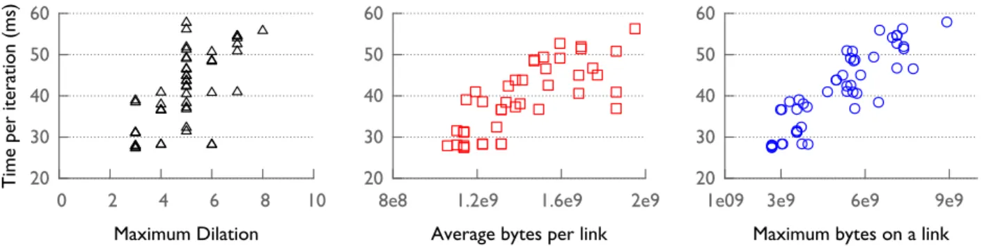
Figure 1: Performance variation with prior metrics for five-point halo exchange on 16,384 cores of Blue Gene/Q. Points represent observed performance with various task mappings. A large variation in performance is observed for the same value of the metric in all three cases.

metric. In contrast, maximum bytes on a link is an experi-mentally obtained metric. In addition to these new metrics, we also use derived metrics that use information only from some outliers (nodes or links).

We present performance predictions using the random-ized forests ensemble method for three different communi-cation kernels: a two-dimensional five-point halo exchange, a three-dimensional 15-point halo exchange, and an all-to-all benchmark over sub-communicators. We show almost perfect correlation for runs on 16,384 and 65,536 cores of Blue Gene/Q. We also show predictions for a production application, pF3D, and for combining samples from differ-ent benchmarks into a single training set and testing set.

In Section 2, we describe the common metrics used in literature and motivate the need for more precise metrics. Sources of contention on torus networks, methodology for collecting hardware counters data, and the proposed met-rics are discussed in Section 3. The benchmarks and super-vised learning techniques used in the paper and the mea-sures of prediction success are described in Section 4. In Sections 5, 6, 7, we present results using prior metrics, new metrics and their combinations. We conclude our work in Section 8.

2. BACKGROUND AND MOTIVATION

Several metrics have been proposed in the literature to evaluate task mappings offline. Let us assume a guest graph,

G= (Vg, Eg) (communication graph between tasks) and a host graph,H = (Vh, Eh) (network topology of the parallel machine). M defines a mapping of the guest graph on the host graph (G on H). The earliest metric that was used to compare the effectiveness of task mappings is dilation [3, 12]. Dilation for a mappingM can be defined as,

dilation(M) = max ei∈Eg

di(M) (1)

where di is the dilation of the edge ei for a mapping M. Dilation of an edge ei is the number of hops between the end-points of the edge when mapped to the host graph. This metric aims at minimizing the length of the longest wire in a circuit [3]. We will refer to this as maximum dilation to avoid any confusion. We can also calculate the average dilation per edge for a mapping as,

average dilation-per-edge(M) = P

ei∈Egdi(M)

|Eg|

(2)

Hoefler and Snir overload dilation to describe the “ex-pected” dilation for an edge and “average” dilation for a mapping [11]. Their definition of expected dilation for an edge can be reduced to equation 1 above by assuming that messages are only routed on shortest paths, which is true for the IBM Blue Gene and Cray XT/XE family (if all nodes are in a healthy state). The average dilation metric, as coined by Hoefler and Snir, is a weighted dilation and has been pre-viously referred to as thehop-bytesmetric by Sadayappan [9] in 1988 and Agarwal in 2006 [2]. Hop-bytes is the weighted sum of the edge dilations where the weights are the message sizes. Hop-bytes can be calculated by the equation,

hop-bytes(M) = X ei∈Eg

di(M)×wi (3) wherediis the dilation of edgeeiandwiis the weight (mes-sage size in bytes) of edgeei.

Hop-bytes gives an indication of the overall communica-tion traffic being injected on to the network. We can derive two metrics based on hop-bytes: the average number of hops traveled by each byte on the network,

average hops-per-byte(M) = P ei∈Egdi(M)×wi P ei∈Egwi (4) and the average number of bytes that pass through a hard-ware link, average bytes-per-link(M) = P ei∈Egdi(M)×wi |Eh| (5) The former gives an indication of how far each byte has to travel on average. The latter gives an indication of the av-erage load or congestion on a hardware link on the network. They are derived metrics (from hop-bytes) and all three are practically equivalent when used for prediction. In the rest of the paper, we use average bytes-per-link.

Another metric that indicates congestion on network links is the maximum number of bytes that pass through any link on the network,

maximum bytes(M) = max li∈Eh

( X

ej∈Eg|ej=⇒li

wj) (6)

where ej =⇒li represents that edgeej in the guest graph goes through edge (link)liin the host graph (network). Hoe-fler and Snir use a second metric in their paper [11], worst

(3)

On link Injection Memory FIFOs (per task)

MU

Memory

Injection Network FIFOs (per node)

Network

Device

Source node

Network Device

Receiver

Buffers based on channels, next link etc.

Intermediate router/switch

MU

Reception Memory FIFOs (per task)

Memory

Reception Network FIFOs (per node)

Network

Device

Destination node

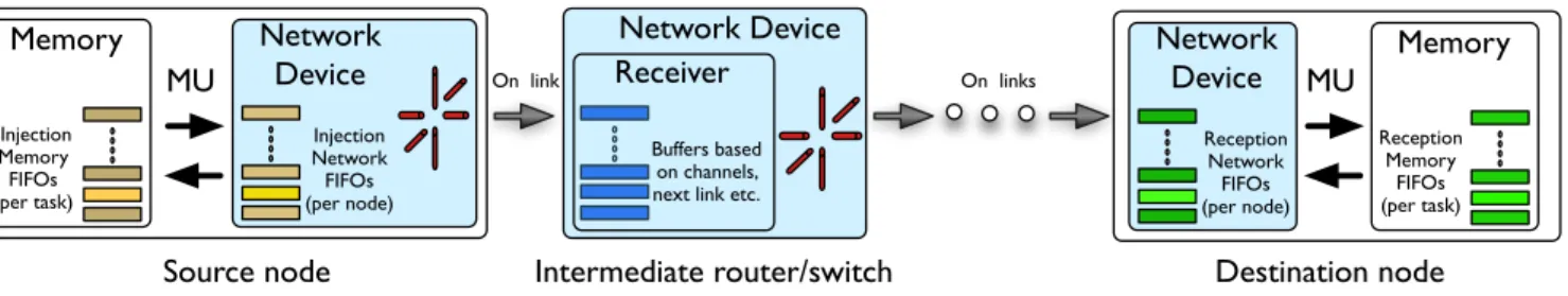
On links

Figure 2: Message flow on Blue Gene/Q - a task initiates a message send by putting a descriptor in one of its memory injection FIFOs; the messaging unit (MU) processes these descriptors and injects packets into the injection network FIFOs from which the packets leave the node via links. On intermediate switches, the next link is decided based on the destination and the routing protocol; if the forward path is blocked, the message is stored in buffers. Finally on reaching the destination, packets are placed in network reception FIFOs from where the MU copies them to either the application memory or memory reception FIFOs.

case congestion, which is the same as equation 6 above. We conducted a simple experiment with three of these metrics described above – maximum dilation, average bytes-per-link and maximum bytes on a link to analyze their cor-relation with application performance. Figure 1 shows the communication time for one iteration of a two-dimensional halo exchange versus the three metrics in different plots. Each point in these plots is representative of a given task mapping on 16,384 cores of Blue Gene/Q. We observe that although the coefficient of determination values (R2_{, metric}

used for prediction success) are high, there is a significant variation in the y-values for different points with the same x-value. For example, in the maximum bytes plot (right), forx= 6e9, there are mappings with performance varying from 20 to 50 ms. These variations make predicting perfor-mance using simple models with a reasonably high accuracy (±5% error) difficult. This motivated us to find new met-rics and ways to improve the correlation between metmet-rics and application performance.

3. CONTENTION ON TORUS NETWORKS

Networks withn-dimensional torus topology are currently used in many supercomputers, such as IBM Blue Gene series, Cray’s XT/XE, and K computer. The IBM Blue Gene/Q (BG/Q) system is the third generation product in the Blue Gene line of massively parallel supercomputers. Each node on a BG/Q consists of 16 4-way SMT cores that run at 1.6 GHz. Nodes are connected by a five-dimensional (5D) torus interconnect with bidirectional links that can send and receive data at 2 GB/s. The BG/Q torus supports two shortest-path routing protocols – deterministic routing for short messages (<64 KB by default, configurable) and configurable dynamic routing for large messages.

3.1 Message flow and resource contention

Figure 2 presents the life cycle of a message on BG/Q. The tasks on a node send data on to the network through the Messaging Unit (MU) on the node. Injection mem-ory FIFO (imFifo) is the data structure used to transfer information between the tasks and the MU. To initiate a message send, a task puts a descriptor of the message in one of itsimFifos. Selection of whichimFifoto inject a descrip-tor in is typically based on the difference in coordinates of source and destination. The MU processes the descriptors in theimFifos, packetizes the message data it reads from

the memory (packet size up to 512 B), and injects them into the injection network FIFOs. The descriptor of the mes-sage contains information of the binding that is used by the MU to inject into the appropriate injection network FIFO. In the default setting, there is a one-to-one mapping be-tweenimFifos and injection network FIFOs. This may lead to contention for injection network FIFOs if the distribution of source-destination pairs is such that a particular network injection FIFOs receives more traffic than others.

From the injection network FIFOs, packets are sent over the network based on the routing strategy and the destina-tion. On the network, contention for hardware links is the most common source of performance degradation. When a packet injected on a link reaches an immediate neighbor, the network device decides the next link the packet needs to be forwarded to. If the next link is occupied, the packets are stored in buffers mapped to the incoming link. In the event of heavy contention for links, these buffers may get filled quickly, and prevent the use of the incoming link for data transfer. When packets eventually reach their destination, they are copied by the MU from the reception network

FIFOs to either the receptionmemoryFIFOs or the appli-cation memory. Limited memory bandwidth may prevent the MU from copying the data, and hence reception injec-tion FIFOs and the buffers attached to the corresponding links may get filled. This may lead to blocking of the links for further communication.

3.2 Collecting hardware counters data

We use two methods to collect information that can indi-cate resource contention as described in Section 3.1:

Blue Gene/Q Counters: The Hardware Performance

Monitoring API (BGPM) provides a simple interface for the BG/Q Universal Performance Counter (UPC) hard-ware. The UPC hardware programs and counts performance events from multiple hardware units on a BG/Q node. Using BGPM to control the Network Unit of the UPC hardware, we implemented a PMPI-based profiling tool that records the following information:

• Sent chunks: count of 32-byte chunks sent on a link. Counters used for collecting this information:

PEVT_NW_USER_PP_SENT: user-level point-to-point

32-byte packetchunkssent (includes chunks in transit);

PEVT_NW_USER_ESC_PP_SENT: user-level

(4)

chunks in transit);

PEVT_NW_USER_DYN_PP_SENT:user-leveldynamic

point-to-point 32-byte packet chunks sent (includes chunks in transit);

• Received packets: count of packets (up to 512 B) received on a link. Counter used for collecting this information:

PEVT_NW_USER_PP_RECV: user-level point-to-point

packetsreceived (includes packets in transit). • Packets in buffers on incoming links: count of packets

added across all buffers associated with an incoming link. Counter used for collecting this information:

PEVT_NW_USER_PP_RECV_FIFO: user-level

point-to-point packets in buffers.

Analytical Program: In order to derive information that is not available via counters, we implemented an analyti-cal program to mimic important aspects of the BG/Q work, including the routing scheme and the injection net-work FIFO selection method. We use it to compute the following information:

• Dilation - number of hops (links) traversed by individ-ual messages on the network.

• Messages in network FIFOs - number of messages in-jected in a particular injectionnetworkFIFO.

3.3 Indicators of resource contention

The information collected from hardware counters and the analytical program allows us to define several new metrics (Table 1). Bytes passing through links are used to com-pute average bytes and maximum bytes on links, which are indicators of link contention (these two are prior metrics). Buffer length, which increases as more packets get blocked during communication, is useful for measuring congestion on the intermediate switches. It may also indicate memory contention, since packets gets buffered if available memory bandwidth to the MU is not sufficient to remove packets from the reception network FIFOs (at the destination). Ra-tio of the buffer length to the number of received packets in-dicates the average delay of packets passing through a link. FIFO length, which is also local to nodes, is an indicator of contention for injection network FIFOs, which may reduce the effective message rate.

Indicator Source Derived from Bytes on links? Counters Sent chunks Buffer length† Counters #Packets in buffers Delay per link† Counters #Packets in buffers

di-vided by received packets Dilation? Analytical Shortest-path routing be-tween source and destina-tion

FIFO length† Analytical Based on PAMI source

Table 1: ?Prior and†new metrics that indicate

con-tention for network resources.

4. EXPERIMENTAL SETUP

In this section, we describe the machines and benchmarks used for the experiments, and thescikit package which pro-vides a Python interface for using several machine learning algorithms.

4.1 Machines

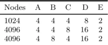
All the experiments were performed on two Blue Gene/Q systems – Mira and Vulcan. Mira is installed at the Argonne National Laboratory and Vulcan is hosted at the Lawrence Livermore National Laboratory. Table 2 presents the possi-ble sizes of the torus dimensions (A, B, C, D and E) when partitions of 1024 and 4096 nodes are requested on BG/Q.

Nodes A B C D E

1024 4 4 4 8 2

4096 4 4 8 16 2

4096 4 8 4 16 2

Table 2: Dimensions of the allocated job partitions on BG/Q.

4.2 Communication kernels

In our experiments, we use three benchmarks that exhibit communication patterns that are commonly seen in HPC applications. By running the benchmarks for four different messages sizes, 8 bytes, 512 bytes, 16 KB and 4 MB, we are able to cover a broad range of communication scenarios typ-ical in large scale scientific applications. In addition, these message sizes also cover different MPI protocols (short, ea-ger, rendezvous), and routing protocols (deterministic and adaptive). All the benchmarks have been implemented in MPI and are described below.

4.2.1 Five-point 2D halo exchange

2D Halo implements the communication pattern of a two-dimensional Jacobi relaxation, which is a common kernel in HPC applications. MPI ranks are arranged in a 2D grid and in each iteration, every MPI rank exchanges one message each with its four nearest neighbors. Performance of this benchmark is measured by taking the average execution time over 100 iterations.

4.2.2 15-point 3D halo exchange

Our second benchmark, 3D Halo, decomposes the MPI ranks into a three-dimensional (3D) grid. In each iteration, every MPI rank communicates with fourteen neighbors (six faces and eight corners) that constitute a 15-point stencil (including itself). 3D Halo differs from 2D Halo in two im-portant aspects: it puts more communication load on the network, and it decomposes MPI ranks into a higher di-mension grid. We use the average execution time for 100 iterations to measure the performance.

4.2.3 All-to-all over sub-communicators

The Sub A2A benchmark is a departure from both 2D Halo and 3D Halo. It performs simultaneous all-to-alls within sub-communicators, and hence is more communica-tion intensive. MPI ranks are decomposed into a 3D grid with sub-communicators of size 64 created along one of its dimensions. Sub A2A has been modeled on codes that per-form FFTs, in which every rank shares data with all other ranks in the same Cartesian sub-grid. The average execution time for 50 iterations is used as the benchmark performance.

4.2.4 Input Data

We use a Python mapping tool, Rubik [6, 13] to gener-ate 84 different task mappings for each of the benchmarks

(5)

MB <= 0.4295

AB <= 0.0082 MB <= 0.4857

AB <= 0.0017 AB <= 0.0176 AB <= 0.1905 leaf

leaf AB <= 0.0021 leaf

Rest of the tree

AB - average bytes MB - maximum bytes

(a) Decision tree. Based on the training set and the learning scheme, conditions are computed to guide pre-diction based on features, e.g., maximum bytes and av-erage bytes. To predict, beginning at the root, the tree is traversed based on the features of a test case until a leaf is reached. The leaf determines the predicted value.

0.0

0.2

0.4

0.6

0.8

1.0 Maximum bytes

0.0

0.2

0.4

0.6

0.8

1.0 Average bytes

Task mapping

Decision surfaces of a random forest

(b) Random forests. A collection of decision trees is used to predict. Each color represent a leaf region in one of the decision trees; regions from different decision trees over-lap. For a test case, all decisions trees are traversed to ob-tain local predictions, which are combined using weights to obtain the final prediction.

Figure 3: Example decision tree and random forests generated using scikit.

and system sizes. Hardware counters data from real runs and data generated by the analytical program for the three benchmarks, four different message sizes, two partition sizes and 84 different task mappings, was used as an input to the machine learning program.

4.3 Prediction using ensemble methods

We employ supervised learning techniques used in statis-tics and machine learning to predict the performance (exe-cution time) of an application for different mappings using metrics described in Section 3.3. The learning algorithm infers a model or function by working with atrainingset that consists ofnsamples(mappings), and one or more in-putfeatures(raw and/or derived such as average bytes) per sample. Each sample has a desired output value (execution time), also known as thetarget. We then use the trained algorithm to predict the output for atestingset (new map-pings for which we wish to predict execution time). The values of the features and the target are normalized to ob-tain the best results.

We tested several supervised learning techniques ranging from statistical techniques, such as linear regression, to ma-chine learning methods, such as support vector mama-chines and decision trees. Thescikit-learn package provides sev-eral of these algorithms/estimators in Python [14]. The two steps, as described previously, are to firstfit the estimator and then to use it topredictunseen samples. For the bench-marks presented in this paper, ensemble learning provided the best fit. Ensemble methods use predictions from several, often weaker models, to produce a stronger model or esti-mator that gives better results than the individual models.

Random forestsare a type of ensemble learning method

developed by Leo Breiman in 2001 [8]. The idea is to build several decision trees and to use averaging methods on these independently built models. In a decision tree, the goal is to create a model that predicts the value of a target vari-able by learning simple decision rules inferred from the data

features. These trees are simple to understand and to inter-pret as they can be visualised easily. However, decision tree based learners create biased trees if some patterns dominate. Random forests attempts to avoid such a bias by adding ran-domness in the selection of condition when splitting a node during the creation of a decision tree. Instead of choosing the best split among all the features, the split that is picked is one among a random subset of the features. Further, the averaging performed on the prediction from independently built decision trees leads to a reduction in the variance and hence an overall better model. We use the

ExtraTreesRe-gressorclass in scikit 0.13.1.

Figure 3 (left) shows an example decision tree that was used in one of our experiments. This tree was produced by training performed using two features, maximum bytes and average bytes, to predict the target, the execution time. The tree shows that at each level, based on the conditions derived from the training set on values of maximum bytes and average bytes, the prediction is guided to reach a leaf node, which determines the target value. Figure 3 (right) presents the overlay of a number of such decision trees over a 2D space spanned by the same two input features. Each color in the figure is a leaf region of one of the decision trees in the random forest generated by fitting the training set. As expected, regions from different decision trees overlap, and cover the entire space. The white circles are the test set being predicted - new mappings with known maximum bytes and average bytes. To predict, all the leaf regions, to which a test case belong, are computed. This provides a set of local predictions for the test case, which are combined to provide a unique target value.

4.4 Metrics for prediction success

The goodness or success of the prediction function (also referred to as thescore) can be evaluated using different met-rics depending on the definition of success. Our main goal is to compare the performance of two mappings and

(6)

deter-10-5 10-4 10-3 10-2 10-1 100 101 Time (s) Mappings 8 bytes 512 bytes 16 KB4 MB (a) 2D Halo 10-5 10-4 10-3 10-2 10-1 100 101 Mappings (b) 3D Halo 10-5 10-4 10-3 10-2 10-1 100 101 Mappings (c) Sub A2A

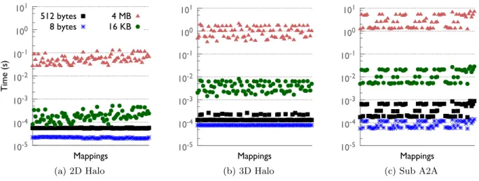
Figure 4: Performance variations with different task mappings on 16,384 cores of BG/Q. As benchmarks become more communication intensive, even for small message sizes, mapping impacts performance.

mine the correct ordering between the mappings in terms of performance. Hence, we focus on a rank correlation metric for determining success; we also present results for a metric that compares absolute values for completeness.

Rank Correlation Coefficient (RCC): Let us assign

ranks to mappings based on their position in two sorted sets (by execution time): observed and predicted perfor-mance. RCC is defined as the ratio of the number of pairs of task mappings whose ranks were in the same pairwise order in both the sets to the total number of pairs. In sta-tistical parlance, RCC equals the ratio of the number of concordant pairs to that of all pairs (Kendall’s Tau [1]). Formally speaking, if observed ranks of tasks mappings are given by{x1, x2,· · ·, xn}, and the predicted ranks by {y1, y2,· · ·, yn}, we define RCC as: concordij=      1, ifxi>=xj&yi>=yj 1, ifxi< xj&yi< yj 0, otherwise RCC= _X 0<=i<n X 0<=j<i concordij /(n(n−1) 2 )

Absolute Correlation (R2): To predict the success for absolute predicted values, we use the coefficient of determi-nation from statistics,R-squared,

R2(y,yˆ) = 1− P i(yi−yˆi) 2 P i(yi−y¯)2

where ˆyi is the predicted value of theith sample, yi is the corresponding true value, and

¯ y= 1 nsamples X i yi

5. PERFORMANCE

PREDICTION

OF

COMMUNICATION KERNELS

In this section, we present results on the prediction of exe-cution times of several communication kernels (Section 4.2)

for different task mappings.

5.1 Performance variation with mapping

Figure 4 presents the execution times for the three bench-marks for four message sizes – 8 bytes, 512 bytes, 16 KB and 4 MB. These sizes represent the amount of data exchanged between a pair of MPI processes in each iteration. For ex-ample, for 2D Halo, this number is the size of a message sent by an MPI process to each of its four neighbors. For a particular message size, a point on the plot represents the execution time (on the y-axis) for a mapping (on the x-axis). For 2D Halo, Figure 4(a) shows that for small messages such as 8 and 512 bytes, mapping has an insignificant im-pact. As the message size is increased to 16 KB, in addition to an increase in the runtime, we observe up to a 7× dif-ference in performance for the best mapping in comparison to the worst mapping (note the logarithmic scale on the y-axis). Similar variation is seen as we further increase the message size to 4 MB. For a more communication intensive benchmark, 3D Halo, we find that mapping impacts per-formance even for 512-byte messages (Figure 4(b)). As we further increase the communication in Sub A2A, the effect of task mapping is also seen for the 8-byte messages as shown in Figure 4(c). In the following sections, we do not present results for the cases where the performance variations from mapping are statistically insignificant: 8- and 512-byte re-sults in case of 2D Halo and 8-byte rere-sults in case of 3D Halo.

5.2 Prior features

We begin with showing prediction results using prior met-rics/features (described in Section 2) and quantify the good-ness of the fit or prediction using rank correlation coefficient (RCC) and R2 (Section 4.4). Figure 5 (top) presents the RCC values for predictions based on prior features (maxi-mum dilation, average bytes per link and maxi(maxi-mum bytes on a link). In most cases, we find that the highest value for RCC is 0.91, i.e., the pairwise ordering of 91% of map-ping pairs was predicted correctly. For a testing set of 28 samples, an RCC of 0.91 implies incorrect prediction of the pairwise ordering of 38 mapping pairs. A notable exception is the 512-byte case for 3D Halo where the RCC is 0.96. In

(7)

0.6 0.7 0.8 0.9 1.0 RCC

Rank correlation coefficient

0.6 0.7 0.8 0.9 1.0 16K 4M 512 16K 4M 8 512 16K 4M R 2

Absolute performance correlation

max dilation

avg bytes max bytes

Sub A2A 3D Halo

2D Halo

Figure 5: Prediction success based on prior features on 16,384 cores of BG/Q. The best RCC score is 0.91 for most cases - 38 mispredictions out of 378.

contrast, for 16 KB message size, the highest RCC is only 0.86.

In the case of 2D Halo and 3D Halo, prediction using max-imum bytes on a link has the highest RCC while prediction using maximum dilation performs very poorly with an RCC close to 0.60. However, for Sub A2A, prediction using aver-age bytes per link is better than prediction using maximum bytes on a link for small to medium message sizes (by 4-5%). The metric for absolute performance correlation,R2, is also shown in Figure 5. For all benchmarks and message sizes, maximum bytes on a link performs the best with a score of up to 0.95 for 3D Halo and Sub A2A. These results substan-tiate the use of maximum bytes and average bytes as simple metrics that are roughly correlated with performance.

5.3 New features

We propose new metrics/features based on the buffer length, delay and FIFO lengths (see Table 1) and derive others by extracting counters and analytical data for outlier nodes and links:

Average Outliers (AO) We define a node or link as an

average outlier if an associated value for it is greater than the average value of the entire data set. Selection of data points based on the average value helps elim-inate low values that can skew derived features and hide information that may be useful.

Top Outliers (TO) Similar to the average outlier, we can define a node or link to be atop outlierif an associated value for it is within 5% of the maximum value across the entire data set.

We can use these two outlier selection criteria to de-fine metrics that represent the features extracted from out-liers. Among a large set of features that we explored using prior/new metrics in combination with known/new deriva-tion methods, we focus on predicderiva-tion using the following features that had the highest RCC: average buffer length (avg buffer), average buffer length of TO (avg buffer TO),

sum of maximum dilation for AO (sum dilation AO), aver-age bytes per link for AO (avg bytes AO), and the averaver-age bytes per link for TO (avg bytes TO).

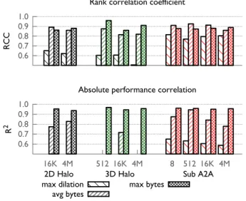
The most important point to note as we transition from Figure 5 to Figure 6 is the general increase in RCC. For Sub A2A in particular, we observe that RCC is consistently 0.95. The previous poor predictions in the case of 16 KB message size for 3D Halo improve from 0.86 to 0.90 (RCC value). For the low traffic 2D Halo, new network-related features such as those based on the buffer length exhibit low correlation. As traffic on the network is increased (larger messages sizes) in 3D Halo and Sub A2A, the RCC of these new network-related features increases, and occasionally sur-passes the RCC of other features.

We note that theR2 value is consistently high only for theavg bytes TO feature. For a number of features, theR2

values are either low or zero. There are two reasons that can explain the lowR2 values: 1) the features did not correlate well with the performance, e.g. avg buffer for 2D Halo and 3D Halo, or 2) the predicted performance followed the same trend as the observed performance but was offset by a factor, e.g.,avg buffer for large messages in 3D Halo.

5.4 Hybrid features

The previous sections have shown that up to 94% pre-diction accuracy can be achieved using a single feature. De-pending on the benchmark and the message size, the feature that provides the best prediction may vary. This motivated us to use several features together to improve the correlation and enable better prediction.

In order to derive hybrid features that improve RCC, we performed a comprehensive search by combining the fea-tures that had high RCC values. In addition, the com-binations of good features were also augmented with fea-tures that exhibited low to moderate correlation with per-formance. We made two important discoveries with these experiments: 1) combining multiple good features may re-sult in a lower accuracy of prediction, and 2) the addition of features that had limited success on their own to good features can boost prediction accuracy significantly.

Hybrid Features combined

H1 avg bytes, max bytes, max FIFO

H2 avg bytes, max bytes, sum dilation AO, max FIFO

H3 avg bytes, max bytes, avg buffer, max FIFO H4 avg bytes, max bytes, avg buffer TO

H5 avg bytes TO, avg buffer TO, avg delay AO, sum hops AO, max FIFO

H6 avg bytes TO, avg buffer AO, avg delay TO, avg delay AO, sum hops A0, max FIFO

Table 3: List of hybrid features that achieve strong correlations.

Figure 7 presents results for the hybrid features that consistently provided high prediction success with different benchmarks and message sizes. Table 3 lists the features that were combined to create these hybrid features. In our experiments, we found that combining the two most com-monly used features,max bytes andavg bytes improves the prediction accuracy in all cases. The gain in RCC was high-est for the 4 MB message size, where RCC increased from

(8)

0.6 0.7 0.8 0.9 1.0 RCC

0.6 0.7 0.8 0.9 1.0 16K 4M 512 16K 4M 8 512 16K 4M R 2

avg buffer

avg buffer TO sum dilation AOavg bytes AO avg bytes TO

Sub A2A 3D Halo

2D Halo

Figure 6: Prediction success based on new features on 16,384 cores of BG/Q. We observe a general increase

in RCC, butR2 values are low in most cases resulting in empty columns.

0.6 0.7 0.8 0.9 1.0 RCC

0.6 0.7 0.8 0.9 1.0 16K 4M 512 16K 4M 8 512 16K 4M R 2

H1 H2 H3 H4 H5 H6

Sub A2A 3D Halo

2D Halo

Figure 7: Prediction success based on hybrid features from Table 3 on 16,384 cores of BG/Q. We obtain

RCC andR2 _{values exceeding 0.99 for 3D Halo and Sub A2A. Prediction success improves significantly for}

2D Halo also.

0.91 (individual best) to 0.94 for all benchmarks. The ad-dition ofmax FIFO, which did not show a high RCC score as a stand alone feature, further increased the prediction accuracy to 0.96. We denote this set as H1.

To H1, we added another low performing feature, avg buffer to obtain H3. This improved the RCC further in all cases with the RCC score now in the range of 0.98−0.99 for 3D Halo and Sub A2A (Figure 7). Replacingavg buffer is this set withavg buffer TO improved the RCC for Sub A2A, but reduced the RCC for 2D Halo. Using a number of such combinations, we consistently achieved RCC up to 0.995 for Sub A2A. Given a testing set of size 28, this implies that the pairwise order of only 2 pairs was mispredicted for Sub A2A; in the worst case for 2D Halo, pairwise order of

16 pairs was mispredicted.

Prediction using hybrid features also results in high R2

values as shown in Figure 7. For 2D Halo, the scores go up from 0.95 and 0.93 to 0.975 and 0.955 for the 16 KB and 4 MB message sizes respectively. For the more communica-tion intensive benchmarks, we obtainedR2values as high as 0.99 in general. Hence, the use of hybrid features not only predicts the correct pairwise ordering of mapping pairs but also does so with high accuracy in predicting their absolute performance.

5.5 Results on 65,536 cores

Figure 8 shows the prediction success for the three bench-marks on 65,536 cores of BG/Q. From all the previously

(9)

pre-0.6 0.7 0.8 0.9 1.0 RCC

0.6 0.7 0.8 0.9 1.0 16K 4M 512 16K 4M 8 512 16K 4M R 2

max bytes

avg bytes TO H3 H5

Sub A2A 3D Halo

2D Halo

Figure 8: Prediction success: summary for all benchmarks on 65,536 cores of BG/Q. Hybrid metrics show high correlation with application performance.

0.01 0.1 1

0 5 10 15 20 25 30

Execution Time (s)

Mappings sorted by actual execution times Blue Gene/Q (65,536 cores) 2D Halo Observed 2D Halo Predicted 1 10 100 0 5 10 15 20 25 30 Execution Time (s)

Mappings sorted by actual execution times Blue Gene/Q (65,536 cores) Sub A2A Observed

Sub A2A Predicted 3D Halo Observed3D Halo Predicted

Figure 9: Summary of prediction results on 65,536 cores using4MB messages. For all benchmarks, prediction

is highly accurate both in terms of ordering and absolute values.

sented features (prior, new and hybrid), we selected the ones with the highest RCC scores for 16,384 cores, and present only those in this figure. Similar to results on 16,384 cores, we obtain significant improvements in the prediction scores using hybrid features in comparison to individual features such asmax bytesandavg bytes TO. For Sub A2A, RCC im-proved by 14% from 0.86 to 0.98, with a RCC value of 1.00 for both 512 bytes and 4 MB message sizes. For 2D Halo and 3D Halo, an improvement of up to 8% was observed in the prediction success. Similar trends were observed forR2

values.

Figure 9 presents the scatter-plot of predicted perfor-mance for the three benchmarks for the 4 MB message size. On the x-axis are the task mappings sorted by observed performance, while the y-axis is the predicted performance. The feature setH5: avg bytes TO, avg buffer TO, avg delay AO, sum hops AO, max FIFO was used for these predic-tions. It is evident from the figure that an almost perfect performance based ordering can be achieved using predic-tion for all three benchmarks, as expected based on the high RCC values. In addition, as shown in Figure 9, absolute

performance values can also be predicted accurately using the proposed hybrid metric. In particular, for Sub A2A with large communication volume, the predicted value curve com-pletely overlaps with the observed value curve. These results suggest that the same set of features correlate with the per-formance irrespective of the system size being used.

6. COMBINING ALL TRAINING SETS

In the previous section, we presented high scores for pre-dicting performance of the three benchmarks using hybrid metrics. For the prediction of individual benchmarks, the training and testing sets were generated using 84 different mappings of the same benchmark for a particular message size on a fixed core count. In this section, we relax these requirements, and explore the space where the training and testing sets are a mix of different benchmarks, message sizes and core counts.

6.1 Combining samples from different

bench-marks

(10)

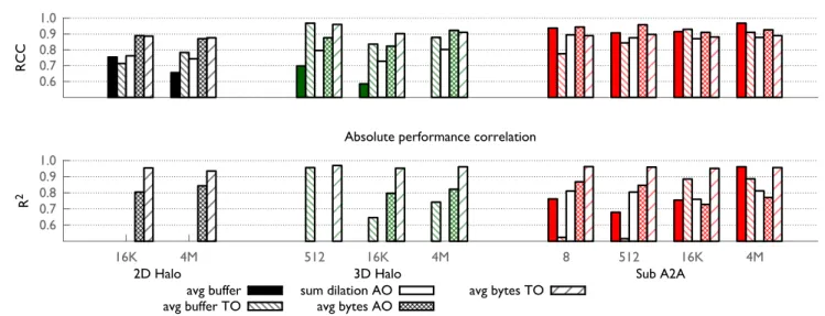
0.6 0.7 0.8 0.9 1.0 RCC

0.6 0.7 0.8 0.9 1.0

avg bytesmax bytessum dilation AOavg bytes TOavg bufferH1 H3 H4 H5 H6

R

2

Absolute Performance Correlation

Figure 10: Prediction success using combination of benchmarks as training and testing sets on 16,384 cores of BG/Q. 1 1e1 1e2 1e3 1e4

Number of mispredictions

Pairwise ordering misprediction

Figure 11: Ordering misprediction using combina-tion of benchmarks as training and testing sets on 16,384 cores of BG/Q. Ordering of only 70 pairs among 14,072 pairs is incorrect in the best case.

are a combination of all three benchmarks with 16 KB and 4 MB message sizes. It is to be noted that the training and testing sets are now six times the size of individual sets (336 vs. 56 for the training set and 168 vs. 28 for the testing set). Figure 10 presents the prediction success for this experiment using prior, new and hybrid features with best correlation.

High RCC values, such as 0.97 foravg bytes, suggests that the combination of training sets results in a better predic-tion than the individual cases. Absolute number of mis-predictions, presented in Figure 11, is close to the sum of mispredictions for individual cases (that are combined to form these sets) for a given metric. This suggests that the presented technique was successful in classifying the sample data from different kinds of communication patterns and message sizes, and in making good predictions using them.

0.6 0.7 0.8 0.9 1.0 RCC

0.6 0.7 0.8 0.9 1.0

avg bytesmax bytessum dilation A0avg bytes TOavg bufferH1 H3 H4 H5 H6

R

2

Absolute Performance Correlation

Figure 12: Predicting performance on 65,536 cores using 16,384 cores. RCC of up to 0.975 was achieved - 3,200 mispredictions in 1,26,756 pairs (2.5%).

These results indicate that if a large database consisting of different communication patterns and message sizes is cre-ated, predicting performance of different classes of appli-cations (possibly with unknown communication structure) may be feasible. We leave an in-depth study of this aspect for future work.

6.2 Predicting performance on 65,536 cores

using 16,384-core samples

We also experimented with predicting the performance on 65,536 cores using the data from runs on 16,384 cores as the training set. The testing set consists of all the benchmarks with message sizes as 16 KB and 4 MB on 65,536 cores, while the training set is the same benchmarks run on 16,384 cores. As shown in Figure 12, we obtained high RCC values for many features. The maximum RCC value of 0.975 was observed using the hybrid feature set H3: avg bytes, max bytes, avg buffer, max FIFO. In terms of absolute number of pairs with incorrect predicted ordering, ordering of∼3,200 pairs were mispredicted among a full set of 1,26,756 pairs.

We find these results to be very encouraging since a strong correlation for predicting performance on large node counts using data from smaller jobs may provide a scalable method for performance prediction. Using smaller systems to predict performance at scale has several advantages. First, generat-ing data sets is more feasible in this regime because it con-sumes less resources. Second, manually generating various mappings for large systems is impractical, but using predic-tion based on runs on smaller node counts, a large number of mappings can be explored with low overhead.

7. RESULTS WITH PF3D

pF3D [17] is a multi-physics code used for studying laser plasma-interactions in the National Ignition Facility (NIF) experiments at LLNL. pF3D is a communication-heavy

(11)

ap-plication and has been shown to benefit significantly from task mapping on Blue Gene/P [6]. This is the first attempt at mapping pF3D on Blue Gene/Q.

pF3D simulations consist of three distinct phases: wave propagation and coupling, advecting light, and solving the hydrodynamic equations. The MPI processes are arranged in a 3D Cartesian grid and all of the MPI communication is performed along different directions (X, Y, Z) of this grid. Wave propagation and coupling consists of two-dimensional (2D) Fast Fourier Transforms (FFTs) inXY-planes; the 2D FFTs are performed via two non-overlapping 1D FFTs along theXandY directions usingMPI_Alltoall. The advection phase involves planar exchange of data with neighbors in the Z-direction performed using MPI_Send and MPI_Recv. Finally, the hydrodynamic phase consists of near-neighbor data exchange in the positive and negativeX,Y andZ direc-tions. The FFT phase and the planar exchange in Z account for most of the time spent in communication in pF3D. The logical 3D grid of processes used for pF3D in this paper was 16×8×128.

In Figure 13, we present RCC scores for predicting the performance of pF3D on 16,384 cores of BG/Q. Whileavg byteshas a very low RCC,max bytes correctly predicts the pairwise ordering for 91% of the task mapping pairs. Inter-estingly, sum of dilations for messages that belong to the average outlier set exhibits a high RCC of 0.94. Similar to the benchmarks, the hybrid features show strong correlation with performance, and have RCCs exceeding 0.96 for this production application. The highest correlation achieved is for the hybrid set H6: avg bytes TO, avg buffer AO, avg delay TO, avg delay AO, sum hops A0, max FIFO that has an RCC of 0.995. TheR2 _{values are significantly lower, in}

contrast with the benchmarks. Formax bytes, theR2value is only 0.76 which increases dramatically to 0.931 for the hybrid setH6.

Figure 14 summarizes the prediction results for pF3D on 16,384 cores using a scatter-plot of observed and predicted values. While the ordering of mapping is correctly predicted, the absolute values are significantly different for many map-pings. As we scaled up to 65,536 cores, we found more irreg-ularities between absolute values of predicted and observed performance. Moreover, the RCC values for known met-rics were found to be as low as 0.52 on 65,536 cores. Us-ing the new and hybrid metrics, the RCC values increased to 0.75 (45% improvement). These RCC values are signif-icantly smaller in comparison to other results presented in this paper. As part of future work, we plan to research fur-ther on possible cause of such a divergence.

8. CONCLUSION

Significant time and effort wasted in real runs to eval-uate the performance of different task mappings suggests the use of simulation or metrics to predict application per-formance offline. Metrics used previously in literature fall short in providing strong correlation with execution time. In this paper, we demonstrate the use of machine learning techniques to obtain high correlation between new metrics and performance of parallel applications for different task mappings.

In addition to prior metrics, such as maximum bytes, we have proposed new metrics, such as buffer length and mes-sages in injection FIFOs, to include the effects of contention for network resources other than links. Using a

combina-0.6 0.7 0.8 0.9 1.0 RCC

0.6 0.7 0.8 0.9 1.0

R

2

Figure 13: Prediction success for pF3D using a va-riety of prior, new, and hybrid metrics. RCC values are very high for the hybrid metrics, as in previ-ous examples, but are somewhat lower for prior and

new single metrics. R2 values are lower on average

overall. 22 23 24 25 26 27 28 29 30 31 0 5 10 15 20 25 30 Execution Time (s)

Mappings sorted by actual execution times Blue Gene/Q (16,384 cores)

pF3D Observed pF3D Predicted

Figure 14: Comparing predicted values with

ob-served values for pF3D on 16,384 cores. Highly ac-curate ordering of mappings is obtained.

tion of these metrics, which includes average and maximum bytes on links, maximum messages contending for an injec-tion FIFO, and the average number of packets in buffers, we show rank correlation coefficients of up to 0.99, i.e. for only 1% of pairs the pairwise ordering is predicted incorrectly. This signifies an improvement of 14% in the prediction suc-cess for an all-to-all over sub-communicators benchmark and 8% for 2D and 3D halo exchange. In addition, prediction using such hybrid metrics also shows highR2 _{scores which}

indicates good prediction in terms of absolute values. Identi-fying these metrics is a step towards accurate offline analysis of task mappings to find the best performing mapping. The next step is to develop techniques to compute metrics that

(12)

are obtained via real runs in this paper, using simulation and/or analysis.

We also successfully attempted combining of training and testing sets from different benchmarks and still retained high prediction accuracy. This suggests that if a large database consisting of different communication patterns and message sizes is created, predicting performance of different classes of applications (possibly with unknown communication struc-ture) may be feasible. More importantly, we show that using training sets from small core counts, we can predict perfor-mance at a larger count with an RCC value of 0.975. This may provide a scalable method for performance prediction at large scales and for future machines without having to per-form detailed network simulations. Finally, we have demon-strated that supervised learning and ensemble methods can be used to predict performance not only for simple communi-cation kernels but also for complex production applicommuni-cations with several diverse communication phases.

Acknowledgments

This work was performed under the auspices of the U.S. De-partment of Energy by Lawrence Livermore National Lab-oratory under Contract DE-AC52-07NA27344. This work was funded by the Laboratory Directed Research and De-velopment Program at LLNL under project tracking code 13-ERD-055 (LLNL-CONF-635857).

This research used computer time on Livermore Comput-ing’s high performance computing resources, provided under the Laboratory Directed Research and Development Pro-gram. This research also used resources of the Argonne Leadership Computing Facility at Argonne National Lab-oratory, which is supported by the Office of Science of the U.S. Department of Energy under contract DE-AC02-06CH11357.

The authors thank W. Scott Futral (LLNL) and Kalyan Kumaran (ANL) for their help with getting the jobs com-pleted on time on Vulcan and Mira respectively. We also thank Dong Chen, Phil Heidelberger, Sameer Kumar, Jeff Parker and Bob Walkup from IBM for the numerous e-mail exchanges and discussions to improve our understanding of the Blue Gene networks.

9. REFERENCES

[1] Kendall tau rank correlation coefficient.

http://en.wikipedia.org/wiki/Kendall_tau_rank_

correlation_coefficient.

[2] T. Agarwal, A. Sharma, and L. V. Kal´e. Topology-aware task mapping for reducing

communication contention on large parallel machines. InProceedings of IEEE International Parallel and Distributed Processing Symposium 2006, April 2006. [3] Aleliunas, R. and Rosenberg, A. L. On Embedding

Rectangular Grids in Square Grids.IEEE Trans. Comput., 31(9):907–913, 1982.

[4] A. Bhatele.Automating Topology Aware Mapping for Supercomputers. PhD thesis, Dept. of Computer Science, University of Illinois, August 2010.

http://hdl.handle.net/2142/16578.

[5] A. Bhatele, E. Bohm, and L. V. Kale. Optimizing communication for charm++ applications by reducing network contention.Concurrency and Computation: Practice and Experience, 23(2):211–222, 2011.

[6] A. Bhatele, T. Gamblin, S. H. Langer, P.-T. Bremer, E. W. Draeger, B. Hamann, K. E. Isaacs, A. G. Landge, J. A. Levine, V. Pascucci, M. Schulz, and C. H. Still. Mapping applications with collectives over sub-communicators on torus networks. InProceedings of the ACM/IEEE International Conference for High Performance Computing, Networking, Storage and Analysis, SC ’12. IEEE Computer Society, Nov. 2012. LLNL-CONF-556491.

[7] A. Bhatel´e, L. V. Kal´e, and S. Kumar. Dynamic topology aware load balancing algorithms for molecular dynamics applications. In23rd ACM International Conference on Supercomputing, 2009. [8] L. Breiman. Random forests.Machine Learning,

45(1):5–32, 2001.

[9] F. Ercal and J. Ramanujam and P. Sadayappan. Task allocation onto a hypercube by recursive mincut bipartitioning. InProceedings of the 3rd conference on Hypercube concurrent computers and applications, pages 210–221. ACM Press, 1988.

[10] F. Gygi, E. W. Draeger, M. Schulz, B. R. de Supinski, J. A. Gunnels, V. Austel, J. C. Sexton, F. Franchetti, S. Kral, C. W. Ueberhuber, and J. Lorenz. Large-scale electronic structure calculations of high-Z metals on the Blue Gene/L platform.In Proceedings of

Supercomputing 2006, 2006. International Conference on High Performance Computing, Network, Sto rage, and Analysis. 2006 Gordon Bell Prize winner (Peak Performance).

[11] T. Hoefler and M. Snir. Generic topology mapping strategies for large-scale parallel architectures. In Proceedings of the international conference on

Supercomputing, ICS ’11, pages 75–84, New York, NY, USA, 2011. ACM.

[12] S.-K. Lee and H.-A. Choi. Embedding of complete binary trees into meshes with row-column routing. IEEE Trans. Parallel Distrib. Syst., 7:493–497, May 1996.

[13] LLNL. Rubik, a mapping tool for n-dimensional mesh topologies.https://scalability.llnl.gov/

performance-analysis-through-visualization,

2012.

[14] F. Pedregosa, G. Varoquaux, A. Gramfort, V. Michel, B. Thirion, O. Grisel, M. Blondel, P. Prettenhofer, R. Weiss, V. Dubourg, J. Vanderplas, A. Passos, D. Cournapeau, M. Brucher, M. Perrot, and E. Duchesnay. Scikit-learn: Machine learning in Python.Journal of Machine Learning Research, 12:2825–2830, 2011.

[15] Shahid H. Bokhari. On the Mapping Problem.IEEE Trans. Computers, 30(3):207–214, 1981.

[16] Soo-Young Lee and J. K. Aggarwal. A Mapping Strategy for Parallel Processing.IEEE Trans. Computers, 36(4):433–442, 1987.

[17] C. H. Still, R. L. Berger, A. B. Langdon, D. E. Hinkel, L. J. Suter, and E. A. Williams. Filamentation and forward brillouin scatter of entire smoothed and aberrated laser beams.Physics of Plasmas, 7(5):2023, 2000.