This work is licensed under a Creative Commons Attribution 4.0 License.
Tímarit um viðskipti og efnahagsmál www.efnahagsmal.is
Asset Allocation Driven by Liabilities:
Application to the Icelandic Pension System
Guðmundur Magnússon and Sverrir Ólafsson
1Abstract
In conventional portfolio management returns are maximised subject to given risk levels. In this framework the only variables of relevance are risk and returns and their interrelationship as expressed in terms of the efficient frontier. It is increasingly the view of investment managers and regulators that pension fund investment strategies need to take their liabilities into consideration when constructing investment portfolios. In this paper we compare the conventional portfolio management approach to asset allocation which aligns investment strategies to a defined liability index. We consider a numerical example based on the Icelandic public sector pension obligation index. A comparison between the conventional risk-return focused approach and the one that seeks to align investment strategies to liabilities shows that the latter approach provides superior performance on market data covering the historical time period from Jan. 2003 to Jan. 2012. The study shows that the liability driven approach performed better in the market downturn in the second half of 2008. Also, a portfolio constructed around liabilities recovered quicker in the years following the market crash.
JEL classification: C61;C65.
Keywords:Asset-Liability management; Mean-Variance optimisation; Pension liabilities; Pension assets; Surplus optimisation.
1
Introduction
Pension funds play a hugely important role in today’s modern societies. They manage people’s life savings, the money they have accrued over their working life, and plan to spend in their retirement years. These accrued savings are managed by fund managers who seek to invest it in a suitable manner. Here, the well-being of so many depends on the performance of so few. The responsibility of the fund managers is substantial and it is paramount that they possess the knowledge and the experience to effectively tackle the fund management tasks.
1 Guðmundur Magnússon has an MSc in financial engineering from Reykjavík University. Sverrir
Ólafsson has a PhD in mathematical physics and is a professor of financial engineering in the Faculty of Science and Engineering at Reykjavík University. E-mail: sverriro@ru.is
Pension assets have been invested in various market instruments, ranging from cash and government bonds across equity to derivatives and complex securitized obligations. Investments in off market enterprises, such as start-ups and hedge funds are not uncommon. The success of the investments impacts on the well-being of the members of the pension fund, either at present through reduced fund contributions or in the retirement years through higher pensions.
Investing in capital and equity markets carries risks, which on occasions can become very substantial. However, the assumption behind market investments has generally been that in the long run risks are moderate to low and returns fairly stable. In between however markets suffer the occasional turmoil which temporarily may set fund values substantially back. After drops in market values recovery can take some time.
Many share the opinion that in recent years equity markets have become too volatile for them to be an acceptable investment alternative for pension funds. Two equity market shocks have occurred since the high-tech bubble burst in late 2000 and a number of economies have still not recovered fully from the 2008 crisis. During this time many pension funds have not managed to cover their liabilities. As a result they have been criticized for being too heavily invested in equities, irrespective of their liability structure and their ability to bear the equity-risk (Ryan & Fabozzi, 2002; Fabozzi, Focardi & Jonas, 2004; Martellini, 2006). Declining values of equities have resulted in falling pension assets while at the same time, decrease in interest rates has pushed up the pension liabilities along with lowering yields on the low-risk fixed income asset classes. The low interest rate environment, combined with the poor performance of global stock markets, has lowered the funding status of many pension plans even further (Martellini, 2006).
The adverse market events occurring in the last two decades have shed light on the weaknesses of risk management and asset allocation practices in the pension fund industry. It is increasingly being recognized among academics and practitioners that pension fund risk management needs some rethinking and that an extensive analysis of what went wrong and how the pension fund industry could adapt to the more volatile and globally connected markets is required (Ryan & Fabozzi, 2002).
As a consequence of the increasing frequency and magnitude of pension plan deficits, the regulatory environment of pension funds has been altered in many countries. More emphasis has been put on managing pension assets in line with estimated liabilities and greater focus has also been put on active risk management. This has increased the need for proper modelling techniques (Fabozzi, Focardi & Jonas, 2004; Martellini, 2006) and puts greater demand on pension fund managers.
The asset allocation of pension funds needs to be guided by its aim to provide returns that dominate the returns of the liability index, at an acceptable risk level. Viewed this way the core role of asset allocation modelling is to better manage uncertainty and to provide a tool for making important investment decisions. Modelling helps in managing uncertainty and suggests actions aimed at achieving return levels at acceptable risk levels. In the pension fund industry, the growing importance of modelling is being recognized although the capabilities of implementing modelling techniques vary between and within countries and pension funds (Fabozzi, Focardi & Jonas, 2004).
The foundation of modern portfolio theory is based on Markowitz‘s famous article, Portfolio Theory (Markowitz, 1952). In his article, Markowitz introduced the idea of risk-return representation of portfolios, where the set of efficient portfolios could be represented via expected return and volatility. He showed that volatility of returns should be minimized,
given some level of expected returns, or equivalently, expected returns should be maximized for given levels of volatility. The total asset risk is reduced by increasing the number of assets in a portfolio and by choosing the assets with respect to cross-correlation of asset returns. Although the systematic risk of the markets cannot be eliminated by diversification, specific asset risk can be reduced by increasing the number of assets held in the portfolio.
By extending the traditional mean variance framework to take account of liabilities, one focuses on growing the pension asset portfolio in excess of the liability portfolio, i.e. achieving pension plan surplus. The pure surplus is generally defined as the total asset value being held by an investor, net of liabilities. As the investment problem is now affected by the presence of liabilities, the investor‘s strategy is not a traditional asset allocation problem, since the investment decisions must enable the investor to cover future liabilities without excessive risk of falling short of this goal. The objective of the problem has transferred into maintaining the value of assets above the value of liabilities, irrespective of actuarial or accounting rules used to calculate the present value of the liabilities. The investment problem has now been transferred from portfolio risk-return space into surplus risk-return space, where fluctuations in the funding ratio, i.e. the ratio of present value of assets to present value of liabilities, have emerged as units of financial risk.
Many practitioners in the pension fund industry have been somewhat reluctant to take full account of liabilities into the mean-variance framework and still favour the traditional Markowitz approach in absence of liabilities (Fabozzi, Focardi & Jonas, 2004). However, an increasing number of practitioners in the pension fund industry and regulatory bodies are slowly accepting the importance of considering liabilities in the investment process. Investors are frequently focused on the return on assets rather than the return on assets net of liabilities and as a consequence, the surplus risk might be undetected. On many occasions, it’s likely that the different dynamics of assets and liability returns are involved in generating an imbalance between assets and liabilities for many pension plans. As an initial step towards considering liabilities in the investment process, models with strong link to standard theory provide simple and straight forward extensions to the widely applied risk-return analysis. In fact, the traditional mean-variance optimisation model is a special case of the surplus optimisation model, where the liabilities are ignored.
The main contribution of this work is to consider four different asset allocation strategies for a hypothetical Icelandic pension fund with liabilities defined by the pension obligation index for employees in the Icelandic public sector. The four asset allocations are derived from the optimisation of four different Lagrangians. Two of the Lagrangians are based on versions of mean variance optimisation where one of the portfolios minimises the surplus return variance (inclusion of liabilities) and the other the asset return variance (no inclusion of liabilities). The other two cases start with Lagrangians where some minimum expected return is fixed, in one case with the inclusion of liabilities and in the other case without liabilities. Accordingly, the four portfolios can be classified into minimum variance portfolios and portfolios with a fixed expected return. This allows for a comparison between those two classes of portfolios along with a comparison between asset allocations that take account of liabilities and those who do not. We consider eight different asset classes, four denominated in USD and four denominated in Icelandic Krona (ISK). They include foreign and domestic equity and bond indexes, as well as private equity and hedge fund indices. The data used spans the period from 1 January 2003 to 1 January 2012 and includes therefore the severe market downturns in the second half of the year 2008.
The article is structured as follows. In section two we give a very brief summary of basic portfolio theory, followed in section three by a discussion of how liabilities can be included. In section four we discuss the data sets used and in section five we analyse and compare the results of the four different allocation strategies. In the final section we summarise and discuss the results and make some suggestions for future research.
2
The classical portfolio model
Consider a portfolio of n risky assets, which at time t have market prices given by
t
S ti
i1,...,nS . With x
t
x ti
i1,...,n presenting the position (number of shares) ineach of the assets the value of the portfolio is given by,
1 n T i i i P t x t S t t t
x S .Let dS ti
S ti
dt
S ti
present the change in the value of the i-th asset over the time interval t t, dt. Then, r ti
dS ti
/S ti
presents the return on the i-th asset over the same time interval. The portfolio return can be written as,
1 n T P i i i R t w t r t t t
w rwhere w
t
w ti
i1,...,n, and w ti
x t S ti
i /P t
. Clearly the w–weights arenormalised since ewT 1, with
1,...,
1i i n
e . Let C
Ci j i j, , 1,...,n be the covariance matrixfor the asset returns. Then the portfolio variance is given by, 2 , , 1 n T P i i j j i j wC w
wCwA conventional approach to the mean-variance portfolio optimisation is to minimise the portfolio variance, subject to different constraint conditions such as the normalisation of weights ewT 1, the required portfolio return levels, T
c
r wr or the presence of liabilities, which the asset allocation is seeking to cover.
3
Inclusion of liabilities
It is assumed that both assets and liabilities follow stochastic processes indicated by P t
and
L t respectively. The returns on assets and liabilities, over the time interval t t, dt, are
P
R t dP t P t and R tL
dL t L t
respectively. We follow (Sharpe and Tint, 1990)and introduce the -scaled surplus value, S t
P t
L t
, where takes values between zero and one. The variable allows us to control the level to which liabilities can be included. If full consideration is taken of the liabilities, on the other hand, by putting noconsideration is taken of liabilities. We define the scaled surplus return with respect to assets (Keel and Muller, 1995)
, S dS t P L R t R t R t P t F t where the funding ratio is defined as F t
P t L t
. The variance of the scaled surplus return is 2 2 2 2 , 2 , S VAR RP FRL P F L F P P L L where P and L are the returns standard deviations of asset portfolio and liabilities
respectively and P L, is the return correlation between assets and liabilities.
4
The portfolio optimisation
We now have the necessary foundation to motivate the construction of four different Lagrangian functions, each one upon optimisation leading to different asset allocations. The four different cases are now briefly introduced. For a more detailed discussion of these four cases see (Magnússon, 2014).
4.1
Minimum return variance portfolio (MVP)
This portfolio arises through the minimisation of the asset portfolio variance 2
P
subject only to the normalisation of the asset allocation vector w, i.e. ewT = 1. The Lagrangian takes the
following form,
1
T T
MVP
L wCw ew
Optimisation leads to well-known asset allocation (Markowitz, 1952). 1 1 MVP T eC w eC e We refer to this as the MVP-portfolio.
4.2
Minimum surplus return variance portfolio (MSVP)
In this case the objective is to minimise the scaled surplus variance, subject only to the normalisation of asset allocation. The resulting Lagrangian has the form,
2 2 2 2 1 T T T MSVP L L L F F wCw w ew where
L i, i1,...,n
i i L L,
i1,...,n
i L, i1,...,n is an n component vector giving thecovariance between the liability index L and individual assets i. Note that LMSVP is the same
This clearly shows that the return variance of the scaled surplus return with respect to assets depends on the return variance of the asset portfolio 2
P
, the return variance of liabilities 2
L
, and the return covariance between the asset components and the liability index,
, ,
1
n
L
i L i P P L L . The objective is to minimize the scaled surplus return variance subject to the normalization of the asset allocation. The result is,
MSVP MVP MSVP
w w
where the additional term satisfies the condition eMSVP 0 and is a measure for the modifications the inclusion of liabilities has on the MVP portfolio without changing its normalisation condition. Furthermore, this modification can be scaled by the parameter. We refer to the resulting asset allocation as the MSVP-portfolio.
4.3
Optimal return portfolio (ORP)
In this case we minimize the return variance of the portfolio assets in the absence of liabilities, subject to asset normalisation and the delivery of some pre-specified returns rc. The resulting
Lagrangian is,
1
T T T
ORP c
L wCw ew rw r
Notice that this is the same Lagrangian as in the MVP case except that now the requirement of portfolio returns of rcis included. That requirement is built into the Lagrangian
by the use of a second Lagrangian parameter . Optimisation of this Lagrangian leads to the following asset allocation,
ORP MVP
w w w
where the correction term satisfies the following condition T 0
ew . We refer to the resulting asset allocation as the ORP-portfolio.
4.4
Surplus optimal return portfolio (SORP)
This portfolio is the same as the MSVP-portfolio with the additional constraint to require a portfolio return of rc. The resulting Lagrangian is,
2 2 2 2 1 T T T T SORP L L c L r F F wCw w ew rw Optimisation results in the following asset allocation,
,
SORP MVP MSVP s
w w w w
where the last term on the right hand side also satisfies the condition ewT,s 0.
We refer to the asset allocation resulting from the optimisation of this Lagrangian as the SORP-portfolio. It is the same as for ORP but contains an additional term stemming from the liabilities. For explicit analytical expressions of the terms MSVP, w and w,s we refer to
(Magnússon, 2014).
Above we have stated four different Lagrangians, only two of which include liabilities. Their optimisation leads to different asset allocations. The important fact is that depending on the constraints added on to the portfolio return variance we end up with different asset allocation strategies, which will tend to perform differently in terms of value, return and risk.
In this short work we discuss the implications of the different constraint conditions for the construction of portfolios and their ability to cover the selected liability index.
As the first two terms in the MSVP and SORP Lagrangians are positive and add together, the surplus return variance can be reduced by selecting the assets in such a way that the covariance between the returns of assets and liabilities are positive. The ratio θ/F plays an important role as it directly affects the variance of surplus returns. That, on the other hand, impacts on the optimal asset allocation in the presence of liabilities. However, the liabilities risk can only be partially hedged in terms of available market securities as the market is not “complete” with respect to liabilities. In other words, liabilities as a random variable cannot completely be replicated in terms of a portfolio of market assets.
An optimal surplus management policy is based on the minimisation of the surplus return variance 2
,
S
and results in an investment in at least two portfolios; a liability hedging portfolio for risk management purposes which is proportional to the ratio θ/F, and the optimal return portfolio which is independent of the ratio θ/F. The latter one is a conventional mean-variance portfolio and represents an “alpha-boosting strategy” in addition to the liability hedge (Merton 1971; Merton 1972; Rudolf & Ziemba, 2004). The funding ratio of a pension fund determines the capability to bear risk and also, in some sense, the need to focus on liabilities. In other words, the higher the funding ratio, the lower the necessity for hedging the liabilities and the pension fund can afford to take more risk by investing in a traditional growth portfolio. For more details see (Magnússon, 2014).
As a practical consequence of the relationship between the funding ratio and liabilities hedge, the hedging policy of pension funds could easily be monitored by the board of the funds governors and the regulatory authorities. This is due to the fact that for optimal portfolios with a fixed θ, only the funding ratio is decisive for the liabilities hedge. From this observation, it can be seen that the funding ratio is directly related to the ability to bear risk. For a specific pension fund, the investment in the liability hedging portfolio thus depends on the funding status and the funding ratio value incorporates the properties that the asset portfolio should have. The lower the funding ratio, the higher should the portion invested in the liability hedge portfolio be as to establish a balanced dynamics between assets and liabilities.
5
The data
The data considered consists of the pension obligation index (POI) for employees in the Icelandic public sector (Numerical Data, Statistics Iceland, 2013), as an index for liabilities, and of eight asset class indices assumed to be representative for the investments available to a hypothetical Icelandic pension funds at the time of the analysis, Table 1. The POI, which is linked to the average salary of public employees in Iceland, is calculated and published on a monthly basis by Statistics Iceland in accordance with act no.1/1997 on pension rights.
Table 1. Indices for liabilities and asset classes
Liabilities Representative Index Currency Source
L: Liability Index Pension obligation index for the ISK Statistics Iceland Icelandic public sector
Asset classes
A1: Dom. Stock Market Index Icelandic All Share Price Index ISK Nasdaq OMX Nordic A2: Foreign Stock Market Index MSCI World Developed Markets USD MSCI Inc.
A3: Hedge Fund Index Barclay Hedge Fund Index USD Barclays Hedge Ltd. A4: Private Equity Index GLPE Private Equity Index USD Red Rocks Capital, LLC A5: Dom. Short Mat. Bond Index 50/50 OMXI3MNI/OMXI1YNI ISK Nasdaq OMX Nordic A6: Dom. Long Mat. Bond Index OMX5YNI ISK Nasdaq OMX Nordic A7: Dom. Indexed Bond Index 50/50 OMXI5YI/OMXI10YI ISK Nasdaq OMX Nordic A8: Foreign Bond Index Vanguard Total Bond Market Index USD The Vanguard Group The eight asset classes consist of four domestic (Icelandic) indices and four foreign indices. Four of these eight asset class indices are bond indices; one foreign and three domestic. The other four are indices representing riskier investments; domestic stocks, foreign stocks, hedge funds and private equity. The returns of the foreign indices are originally all in USD and are recalculated in terms of ISK returns using the official ISK/USD currency rates published by the Central Bank of Iceland.
The OMX Iceland All-Share Index (ICEXI, 2013) includes all the shares listed on Nasdaq OMX Nordic Exchange Iceland. The MSCI World Index (MSCI Index Performance, 2013) is a stock market index, including approximately 2000 securities from 23 countries but excluding stocks from emerging and frontier markets. The hedge fund index data are provided by the Barclay Hedge Ltd. (USA) database. The Barclay Hedge Fund Index (Barclay Hedge Fund Index, 2013) is a measure of the average return of all hedge funds in the Barclay database. The private equity index is the Red Rocks Capital Global Listed Private Equity (GLPE) index (GLPE Index, 2013). The GLPE index is designed to track the performance of private equity firms, which are publicly traded on any nationally recognized exchange worldwide. The domestic short maturity bond index constructed for this analysis is composed of equally weighted returns of two non-indexed bond indices from Nasdaq OMX Nordic; the 3 month OMXI3MNI and the 1 year OMX1YNI indices. The non-indexed 5 year OMX5YNI bond index is used as the domestic long maturity bond index. The inflation linked bond index used is composed of equally weighted returns of two indexed bond indices from Nasdaq OMX Nordic, the 5 year OMXI5YI and the 10 year OMX10YI indices. The foreign bond index is the Vanguard Total Bond Market index. The index is designed to provide broad exposure to U.S. investment grade bonds and consists of approximately 30% in corporate bonds and 70% in U.S. government bonds of all maturities.
Figures 1 and 2 illustrate the monthly prices for all the indices which on 01 January 2003 have been normalised to the price of 100. Figure 1 illustrates the equities and hedge funds (A1- A4) and the liability index. Figure 2 illustrates the four fixed income securities (A5 – A8) and the liability index.
Figure1. Price indices for A1-A4 and L Figure2. Price indices for A5-A8 and L
Table 2. Descriptive statistics for logarithmic returns; Jan. 2003 - Jun. 2008
#Obs: 65 L A1 A2 A3 A4 A5 A6 A7 A8 Mean 0,069 0,204 0,118 0,1 0,236 0,084 0,057 0,082 0,041 Std. Dev. 0,029 0,213 0,118 0,115 0,145 0,012 0,079 0,057 0,119 Skewness 2,393 -0,661 0,422 0,675 0,333 0,772 -0,714 0,111 0,262 Exc. Kurtosis 7,541 3,352 2,606 3,024 2,649 3,36 11,015 4,26 2,447 JB test-statistic 115,041 4,846 2,261 4,709 1,482 6,515 179,237 4,426 1,54 For the comparison analysis, the initial optimal portfolios, constructed in July 2008, are based on return data for the asset classes and liabilities from January 2003 to and including June 2008, consisting of 65 monthly return data points. For further analysis of the return data, Table 2 provides descriptive statistics for the logarithmic returns of the nine time series. The liability returns have a mean growth rate of 6.9% with volatility of 2.9%, indicating a steady growth with small variation.
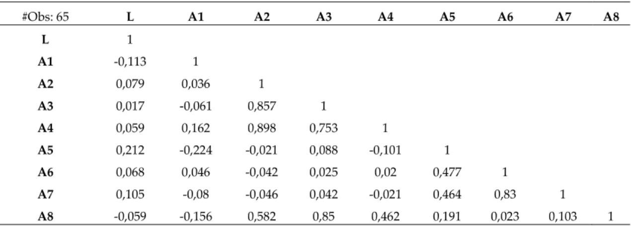
In the considered data none of the return values for the liability index are negative. Accordingly, skewness and excess kurtosis suggest a leptokurtic distribution with positively skewed returns. This is also confirmed by the Jarque-Bera (JB) test (Jarque & Bera, 1987) result which clearly rejects the null hypothesis of a normal distribution for the liabilities returns. The data analysis suggests a leptokurtic distribution for all the asset classes with positively skewed returns, except for domestic stocks and domestic long maturity bonds where the returns are negatively skewed. The JB test rejects the normality hypothesis for the domestic short and long bond indices (A5, A6) and for the liability index.
Return correlation estimates show that returns on all asset classes are positively correlated with the liabilities, except domestic stocks and foreign bonds, Table 3. This shows that six out of the eight asset classes have liability hedging properties. The highest asset-liability correlation is from domestic short maturity bonds, twice as high as in the case of domestic indexed bonds. Foreign stocks and domestic long maturity bonds have the third and fourth highest correlation with liabilities. Foreign bonds have the second lowest return correlation with liabilities, which can be largely explained by currency returns. This is confirmed by a
2003 2004 2005 2006 2007 2008 2009 2010 2011 20120 100 200 300 400 500
600 Prices; Equities and Hedge funds, 01/2003 - 01/2012 A1 A2 A3 A4 L 2003 2004 2005 2006 2007 2008 2009 2010 2011 2012 80 100 120 140 160 180 200 220 240 260
280 Prices; Fixed income securities, 01/2003 - 01/2012 A5
A6 A7 A8 L
simple linear regression where more than 90% of the variability in ISK returns of the foreign bond index is explained by currency returns (Magnússon, 2014).
Table 3. Return correlation estimates for the asset classes and liabilities; Jan. 2003 - Jun. 2008 #Obs: 65 L A1 A2 A3 A4 A5 A6 A7 A8 L 1 A1 -0,113 1 A2 0,079 0,036 1 A3 0,017 -0,061 0,857 1 A4 0,059 0,162 0,898 0,753 1 A5 0,212 -0,224 -0,021 0,088 -0,101 1 A6 0,068 0,046 -0,042 0,025 0,02 0,477 1 A7 0,105 -0,08 -0,046 0,042 -0,021 0,464 0,83 1 A8 -0,059 -0,156 0,582 0,85 0,462 0,191 0,023 0,103 1 The value of the ISK against the USD rose considerably during the period from January 2003 – January 2008, just to decline to almost the 2003 level by the end of June 2008. The returns on foreign securities suffered due to the increase in the ISK/USD rate and low yielding foreign bonds yielded negative returns in ISK for the years 2003 – 2008 as figure 2 implies. During the largest part of this time period, currency returns made most foreign investments unattractive in terms of ISK returns.
6
Comparison analysis
The purpose of this numerical example is to provide a comparative analysis of the surplus generated by mean-variance optimal portfolios in the absence and presence of liabilities. Four portfolio strategies are analysed as possible investment strategies for a hypothetical Icelandic pension fund where the value of its liabilities is assumed to follow the POI. For the optimal allocations in the presence of liabilities, full consideration is given to liabilities by setting the importance parameter .
The comparison analysis covers both optimal allocation strategies constrained to long-only positions and optimal allocation strategies allowing unlimited long-short positions. In many countries, pension funds are not allowed to take short positions and therefore, comparison of long-only portfolio strategies should be the natural choice. On the other hand, a comparison of strategies without any long-only constraints allows for the observation of best possible diversification, size of short positions and liability hedging characteristics.
In order to compare the performance and the surplus generating ability of the optimal asset allocations in absence and presence of liabilities, the allocation strategies are compared to each other and also to the liability index. The four optimal allocation strategies considered are the minimum variance portfolio (MVP), the minimum surplus variance portfolio (MSVP), optimal return portfolios in absence of liabilities (ORP) and surplus optimal return portfolios in the presence of liabilities (SORP). Generally, the return requirements are set at 12% which
might seem to be high but can be explained by the fact that the MVP yields a 9.3% return for the historical period from Jan. 2003 to Jun. 2008. Also, the nominal interest rates and inflation have been higher in Iceland than in other western economies, making the 12% nominal return requirement a reasonable choice.
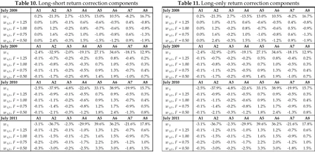
To take an account of the different funding status for the hypothetical pension fund, the comparison is made between four different initial funding ratios; F = [0.50, 0.75, 1, 1.25]. The initial asset allocations for all portfolios are found by using return data from January 2003 to June 2008, Tables 4 – 11, after portfolio re-balancing has been undertaken in July each year. For Tables 4 – 11 see Appendix. In the Tables we indicate them by July 2008 portfolios. The portfolio performance and surplus comparison analysis is undertaken for the remaining historical data period from July 2008 to January 2012 and the annually rebalanced portfolios are indicated by July 2009, July 2010 and July 2011. When portfolios are rebalanced, the most recent historical data is added to the dataset that provides inputs to the optimisation. The allocation process accounts for the funding status of the strategies. Then, the performance of the different asset allocations is compared to each other and to the liability index. In Table 4 we present the long-short MVP and MSVP and in Table 5 the long only MVP and MSVP portfolios. The corrections to the MVP portfolio to achieve the MSVP portfolios are presented in Tables 6 and 7.
In Tables 8 and 9 we present the ORP and SORP portfolios and the associated corrections
w and w,s are presented in Tables 10 and 11. Note that all portfolio corrections add up to
zero as they conserve the normalization of the asset allocation.
The performance of the portfolios with F = 1 and the liability index is illustrated in figures 3 - 4 and the surplus associated with the allocation strategies is shown in figures 5 - 6. In the figures legends, ORP and SORP refer to the optimal portfolio in absence and presence of liabilities with the 12% return requirement, respectively. Figures 7 – 8 present the average surplus generated by the strategies from July 2008 to January 2012.
Considering the long-only and the long-short portfolios separately, the performance patterns for the four strategies are similar for all three funding ratios. In the beginning of the time period under consideration, just before the 2008 market collapse, the performance and the surplus of the MVP indices are just about the same as the MSVPs. When the market downturn starts, in the last quarter of 2008, the MSVP indices show better performance than their MVP counterparts and drop less in value.
The growth rate of the MSVP is, on average, higher than that of the MVP over the whole considered time period from 2009 to 2012 as seen in figures 3 - 4. Also, figures 5 – 6 illustrate that the surplus generated by the MSVP exceeds that of the MVP over the same period. Furthermore, in terms of average surplus generated, the MSVP exceeds the surplus generated by MVP, for the whole time period and for all considered funding levels; Figures 7 – 8.
Similar results are observed when the optimal portfolios in absence (ORP) and presence (SORP) of liabilities are considered. For both portfolios, ORP and SORP, the required return is set at 12%. The SORP portfolios dropped less than the ORP portfolios during the 2008 financial crisis and following that grew faster in the years from 2009 to 2012. Also, in terms of surplus the SORP portfolios performed better than the ORP portfolios over the time period from July 2008 to January 2012. All these results apply equally for long-only and long-short allocation strategies. For both long-only and long-short portfolios and for all three funding ratios, the strategies taking liabilities into account outperform their asset-only counterparts both in terms of average surplus and portfolio values.
Figure 3. Portfolio price indices Jul. 2008-12 Figure 4. Portfolio price indices Jul. 2008-12
Figure 5. Portfolio surplus indices Jul. 2008-12 Figure 6. Portfolio surplus indices Jul. 2008-12
Figure 7. Portfolio average surplus Jul. 2008-12 Figure 8. Portfolio average surplus Jul. 2008-12
When comparing the MSVP and the MVP strategies with the higher return requirement strategies, ORP and SORP, the former generally outperform the latter. However, the actual level of outperformance depends on the portfolio funding ratio, Figure 7 - 8.
2008.5 2009 2009.5 2010 2010.5 2011 2011.5 2012 2012.5 90 95 100 105 110 115 120 125
130 Long-short portfolio indices; F0= 1.0 MSVP MVP SORP ORP Liabilities 2008.5 2009 2009.5 2010 2010.5 2011 2011.5 2012 2012.5 -30 -25 -20 -15 -10 -5 0 5 10 15
20 Long-only portfolio surplus; F0= 1.0 MSVP MVP SORP ORP 2008.5 2009 2009.5 2010 2010.5 2011 2011.5 2012 2012.5 -15 -10 -5 0 5 10 15
20 Long-short portfolio surplus; F0= 1.0 MSVP MVP SORP ORP 1.25 1.00 0.75 F0 -40 -30 -20 -10 0 10 20 30
40 Long-only portfolio average surplus MVP MSVP ORP SORP 1.25 1.00 0.75 F0 -30 -20 -10 0 10 20 30
40 Long-short portfolio average surplus MVP MSVP ORP SORP
The sharp increase in liabilities in 2011 had a negative effect on surplus for all strategies as can be observed as a sharp drop in surplus in the latter part of the year 2011. Nevertheless, the strategies considering liabilities maintain higher surplus than their classic asset-only counterparts as indicated by figures 5 – 8.
One more important observation is that the portfolio strategies that take liabilities into considerations fell less, both in terms of value and surplus, during the 2008 crises. Also, they showed better recovery, again both in terms of value and surplus, in the months and years following the financial crisis.
7
Summary and concluding remarks
In recent years the performance of pension funds has come under much scrutiny. Recent severe market downturns, including the high-tech bubble burst in late 2000 and the 2008 financial crisis have inflicted heavy losses on many pension funds all over the world. These and other market volatilities have fuelled extensive discussions about pension fund asset allocation and risk management strategies. A focal point in these discussions are questions like: Is the cause of losses mainly due to heavy falls in asset prices, mainly equities, or can some blame be put on poor and inappropriate fund management strategies?
In this work we have analysed the performance of eight different asset allocation strategies (portfolios) in covering a pension obligation index (POI) used for some employees in the Icelandic public sector. There are eight different asset classes available for portfolio inclusion; four domestic assets, one based on an equity index and three on different bond indexes. The remaining four asset classes are foreign and all denominated in USD; one equity index, one bond index, a hedge fund index and a private equity index. The time period considered is from 01 January 2003 to 01 January 2012 and includes therefore the severe market downturns in the latter half of the year 2008.
Two of the portfolios do not consider the POI but focus on minimising the portfolio variance subject to some constraint conditions. They are; MVP-portfolio where the portfolio variance is minimised subject to asset normalisation and ORP-portfolio where the portfolio variance is minimised subject to asset normalisation and specified required returns. The remaining two portfolios take the liabilities into consideration. They are; MSVP-portfolio where the surplus variance is minimised subject only to asset normalisation and SORP-portfolio where the surplus variance is minimised subject to asset normalisation and specified required returns. Both long-only and long-short portfolios are considered.
For market data covering nine years, from January 2003 to January 2012, the results of our analysis demonstrate the superiority of the strategies that consider liabilities compared to those that do not. With regard to surplus these results are confirmed in figures 5 - 8. Interestingly, the results also show that the portfolios considering liabilities grow at a higher rate than their no-liabilities counterparts. Also, the inclusion of liabilities supports faster recovery after the 2008 crisis than their counterparts not taking liabilities into account. Since the liability index in this analysis had a stable growth with a low volatility, benchmarking portfolio returns with this liability index resulted in a low-risk investment strategy that suffered less from the 2008 market downswing than the traditional mean-variance strategies.
This might suggest that for periods of market volatility, benchmarking portfolios with steady-growth and low-volatile indices could reduce the negative effects of market downturns.
These results are very promising as they on all fronts lend support to asset allocation strategies that take liabilities into consideration. In some ways this is not surprising as the main focus of all pension funds needs to be on their liabilities as defined by the future pension rights of their members. Focusing on growth portfolios per se, without taking any direct notice of liabilities does not seem to do justice to the expected future needs of those who have provided the capital that is being invested.
The liability index considered in this work is specific and is unlikely to be representative for the liability of other pension funds in Iceland. Therefore, more research into different liability structures is required before any general conclusions can be drawn for the Icelandic and other pension markets. When including liabilities it is very important to get as accurate models of the future liability index as possible. However, the model presented here is entirely generic and therefore any constructed liability index can be used as a possible input. Nevertheless, it is important to realize that as the investment assets are mainly drawn from market instruments the liability index generally depends strongly on demographic variables with only partial and indirect correlation to the market. This will be the focus of another research work to be published in the near future.
References
Barclay Hedge Fund Index. (n.d.). BARCLAY HEDGE, LTD. Retrieved April 4, 2013, from http://www.barclayhedge.com/research/indices/ghs/Hedge_Fund_Index.html
Fabozzi, F. J., Focardi, S. M. & Jonas, C. L. (2004). Can Modeling Help Deal with the Pension Funding Crisis? The Intertek Group.
GLPE INDEX. (n.d.). Red Rocks Capital LLC. Retrieved April 4, 2013, from http://www.redrockscapital.com/?q=glpe-index/returns
ICEXI Quote - Iceland Stock Exchange ICEX Main Index. (n.d.). Bloomberg. Retrieved April 4, 2013, from http://www.bloomberg.com/quote/ICEXI:IND
Jarque, C. M. & Bera, A. K. (1987). A test for normality of observations and regression residuals, International Statistical Review, 55(2), 163–172.
Keel, A. & Muller, H. H. (1995). Efficient Portfolios in the Asset Liability Context, Astin Bulletin, 25(1), 33–48.
Magnússon, G, (2014). Risk-return optimization in the absence and presence of liabilities: comparative solution analysis and related methods, Master of Science Thesis, School of Science and Engineering, Reykjavik University, 1-169
Markowitz, H. (1952). Portfolio Selection, The Journal of Finance, 7(1), 77–91.
Martellini, L. (2006). Managing Pension Assets: From Surplus Optimization to Liability-Driven Investment, EDHEC Risk Management Centre, Nice, 1–42.
Merton, R. C. (1971). Optimal Portfolio and Consumption Rules in a Continuous-time Model. Journal of Economic Theory, 3(4), 373–413.
Merton, R. C. (1972). An Analytic Derivation of the efficient frontier. The Journal of Financial and Quantitative Analysis, 7(4), 1851–1872.
MSCI Index Performance. (n.d.). MSCI Inc. Retrieved April 4, 2013, from
http://www.msci.com/products/indices/country_and_regional/all_country/performance.html
Numerical data, Index of pension scheme commitments for public servants 1997-2013. (n.d.). Statistics Iceland. Retrieved March 20, 2013 from http://www.hagstofa.is/
Rudolf, M. & Ziemba, W. T. (2004). Intertemporal surplus management. Journal of Economic Dynamics and Control, 28(5), 975–990.
Ryan, R J. & Fabozzi, F. J. (2002). Rethinking Pension Liabilities and Asset Allocation. A pension crisis looms. The Journal of Portfolio Management, 28(4), 7–15.
Sharpe, W. F. & Tint, L. G. (1990). Liabilities— A New Approach. The Journal of Portfolio Management, 16(2), 5–10. Vanguard Total Bond Market Index Inv (VBMFX). (n.d.). YAHOO FINANCE. Retrieved April 5, 2013, from
Appendix
July 2008 A1 A2 A3 A4 A5 A6 A7 A8 July 2008 A1 A2 A3 A4 A5 A6 A7 A8 MVP 1.4% -2.0% 104.0% -8.3% 3.3% 1.4% -2.5% 2.8% MVP 1.4% 0.0% 97.4% 0.0% 0.0% 0.0% 0.0% 1.2% MSVP, F = 1.25 -0.3% 1.8% 102.5% -9.4% 8.0% 3.1% -8.0% 2.2% MSVP, F = 1.25 0.0% 0.0% 97.8% 0.0% 0.0% 0.0% 0.0% 2.2% MSVP, F = 1.00 -0.7% 2.7% 102.1% -9.6% 9.2% 3.6% -9.3% 2.1% MSVP, F = 1.00 0.0% 0.3% 97.6% 0.0% 0.0% 0.0% 0.0% 2.1% MSVP, F = 0.75 -1.5% 4.3% 101.5% -10.1% 11.2% 4.3% -11.6% 1.8% MSVP, F = 0.75 0.0% 1.2% 97.1% 0.0% 0.0% 0.0% 0.0% 1.7% MSVP, F = 0.50 -2.9% 7.4% 100.3% -11.0% 15.2% 5.8% -16.2% 1.3% MSVP, F = 0.50 0.0% 3.2% 94.6% 0.0% 1.3% 0.0% 0.0% 0.8% July 2009 A1 A2 A3 A4 A5 A6 A7 A8 July 2009 A1 A2 A3 A4 A5 A6 A7 A8 MVP 0.5% 0.8% 113.9% -15.5% 0.2% 2.5% -1.2% -1.2% MVP 0.0% 0.0% 99.5% 0.0% 0.0% 0.0% 0.5% 0.0% MSVP, F = 1.25 0.6% 5.7% 110.2% -19.2% 8.2% 1.9% -3.3% -4.2% MSVP, F = 1.25 0.0% 0.0% 100.0% 0.0% 0.0% 0.0% 0.0% 0.0% MSVP, F = 1.00 0.6% 6.9% 109.3% -20.1% 10.2% 1.8% -3.8% -4.9% MSVP, F = 1.00 0.0% 0.0% 100.0% 0.0% 0.0% 0.0% 0.0% 0.0% MSVP, F = 0.75 0.6% 8.9% 107.7% -21.6% 13.6% 1.6% -4.7% -6.1% MSVP, F = 0.75 0.0% 0.0% 100.0% 0.0% 0.0% 0.0% 0.0% 0.0% MSVP, F = 0.50 0.7% 13.0% 104.7% -24.7% 20.2% 1.1% -6.5% -8.5% MSVP, F = 0.50 0.0% 0.0% 100.0% 0.0% 0.0% 0.0% 0.0% 0.0% July 2010 A1 A2 A3 A4 A5 A6 A7 A8 July 2010 A1 A2 A3 A4 A5 A6 A7 A8 MVP 1.6% -5.0% 127.2% -20.9% -15.5% 0.9% 9.0% 2.7% MVP 1.5% 0.0% 85.9% 0.0% 0.0% 0.0% 12.5% 0.0% MSVP, F = 1.25 1.7% -1.3% 125.4% -24.4% -9.5% -0.1% 7.9% 0.4% MSVP, F = 1.25 1.3% 0.0% 87.0% 0.0% 0.0% 0.0% 11.7% 0.0% MSVP, F = 1.00 1.7% -0.4% 124.9% -25.3% -8.0% -0.4% 7.6% -0.2% MSVP, F = 1.00 1.3% 0.0% 87.3% 0.0% 0.0% 0.0% 11.4% 0.0% MSVP, F = 0.75 1.7% 1.2% 124.1% -26.8% -5.5% -0.8% 7.2% -1.2% MSVP, F = 0.75 1.2% 0.0% 87.7% 0.0% 0.0% 0.0% 11.1% 0.0% MSVP, F = 0.50 1.8% 4.3% 122.6% -29.7% -0.5% -1.6% 6.2% -3.1% MSVP, F = 0.50 1.0% 0.0% 88.6% 0.0% 0.0% 0.0% 10.4% 0.0% July 2011 A1 A2 A3 A4 A5 A6 A7 A8 July 2011 A1 A2 A3 A4 A5 A6 A7 A8 MVP 1.7% -7.6% 123.7% -23.2% -8.9% 4.0% 7.2% 3.2% MVP 1.5% 0.0% 86.3% 0.0% 0.0% 0.0% 12.1% 0.0% MSVP, F = 1.25 1.8% -4.6% 123.6% -26.4% -5.0% 2.0% 7.5% 1.1% MSVP, F = 1.25 1.3% 0.0% 87.1% 0.0% 0.0% 0.0% 11.6% 0.0% MSVP, F = 1.00 1.8% -3.8% 123.6% -27.2% -4.0% 1.6% 7.5% 0.5% MSVP, F = 1.00 1.3% 0.0% 87.3% 0.0% 0.0% 0.0% 11.4% 0.0% MSVP, F = 0.75 1.9% -2.5% 123.5% -28.6% -2.4% 0.7% 7.6% -0.3% MSVP, F = 0.75 1.2% 0.0% 87.6% 0.0% 0.0% 0.0% 11.2% 0.0% MSVP, F = 0.50 2.0% 0.1% 123.4% -31.2% 0.9% -0.9% 7.8% -2.1% MSVP, F = 0.50 1.0% 0.0% 88.2% 0.0% 0.0% 0.0% 10.8% 0.0%Table 4. Long-short MV asset portfolios Table 5. Long-only MV asset portfolios
July 2008 A1 A2 A3 A4 A5 A6 A7 A8 July 2008 A1 A2 A3 A4 A5 A6 A7 A8 wMVP A1 A2 A3 A4 A5 A6 A7 A8 wMVP A1 A2 A3 A4 A5 A6 A7 A8 ϕMSVP, F = 1.25 1.4% -2.0% 104.0% -8.3% 3.3% 1.4% -2.5% 2.8% ϕMSVP, F = 1.25 1.4% 0.0% 97.4% 0.0% 0.0% 0.0% 0.0% 1.2% ϕMSVP, F = 1.00 -0.3% 1.8% 102.5% -9.4% 8.0% 3.1% -8.0% 2.2% ϕMSVP, F = 1.00 0.0% 0.0% 97.8% 0.0% 0.0% 0.0% 0.0% 2.2% ϕMSVP, F = 0.75 -0.7% 2.7% 102.1% -9.6% 9.2% 3.6% -9.3% 2.1% ϕMSVP, F = 0.75 0.0% 0.3% 97.6% 0.0% 0.0% 0.0% 0.0% 2.1% ϕMSVP, F = 0.50 -1.5% 4.3% 101.5% -10.1% 11.2% 4.3% -11.6% 1.8% ϕMSVP, F = 0.50 0.0% 1.2% 97.1% 0.0% 0.0% 0.0% 0.0% 1.7% July 2009 A1 A2 A3 A4 A5 A6 A7 A8 July 2009 A1 A2 A3 A4 A5 A6 A7 A8 wMVP A1 A2 A3 A4 A5 A6 A7 A8 wMVP A1 A2 A3 A4 A5 A6 A7 A8 ϕMSVP, F = 1.25 3.3% -6.6% 13.5% -4.5% -15.0% -3.3% 15.1% -2.6% ϕMSVP, F = 1.25 0.0% -3.2% 4.9% 0.0% -1.3% 0.0% 0.5% -0.8% ϕMSVP, F = 1.00 3.4% -1.7% 9.8% -8.2% -7.0% -3.8% 12.9% -5.5% ϕMSVP, F = 1.00 0.0% -3.2% 5.4% 0.0% -1.3% 0.0% 0.0% -0.8% ϕMSVP, F = 0.75 3.5% -0.5% 8.9% -9.1% -5.0% -4.0% 12.4% -6.2% ϕMSVP, F = 0.75 0.0% -3.2% 5.4% 0.0% -1.3% 0.0% 0.0% -0.8% ϕMSVP, F = 0.50 3.5% 1.5% 7.4% -10.6% -1.7% -4.2% 11.5% -7.4% ϕMSVP, F = 0.50 0.0% -3.2% 5.4% 0.0% -1.3% 0.0% 0.0% -0.8% July 2010 A1 A2 A3 A4 A5 A6 A7 A8 July 2010 A1 A2 A3 A4 A5 A6 A7 A8 wMVP A1 A2 A3 A4 A5 A6 A7 A8 wMVP A1 A2 A3 A4 A5 A6 A7 A8 ϕMSVP, F = 1.25 0.9% -18.0% 22.6% 3.8% -35.7% -0.2% 15.5% 11.2% ϕMSVP, F = 1.25 1.5% 0.0% -14.1% 0.0% 0.0% 0.0% 12.5% 0.0% ϕMSVP, F = 1.00 1.0% -14.3% 20.7% 0.3% -29.7% -1.2% 14.4% 8.9% ϕMSVP, F = 1.00 1.3% 0.0% -13.0% 0.0% 0.0% 0.0% 11.7% 0.0% ϕMSVP, F = 0.75 1.0% -13.4% 20.2% -0.6% -28.2% -1.4% 14.1% 8.3% ϕMSVP, F = 0.75 1.3% 0.0% -12.7% 0.0% 0.0% 0.0% 11.4% 0.0% ϕMSVP, F = 0.50 1.0% -11.9% 19.4% -2.0% -25.7% -1.8% 13.6% 7.4% ϕMSVP, F = 0.50 1.2% 0.0% -12.3% 0.0% 0.0% 0.0% 11.1% 0.0% July 2011 A1 A2 A3 A4 A5 A6 A7 A8 July 2011 A1 A2 A3 A4 A5 A6 A7 A8 wMVP A1 A2 A3 A4 A5 A6 A7 A8 wMVP A1 A2 A3 A4 A5 A6 A7 A8 ϕMSVP, F = 1.25 -0.1% -11.9% 1.1% 6.5% -8.4% 5.5% 1.0% 6.4% ϕMSVP, F = 1.25 0.5% 0.0% -2.3% 0.0% 0.0% 0.0% 1.8% 0.0% ϕMSVP, F = 1.00 0.0% -8.8% 1.0% 3.3% -4.5% 3.6% 1.2% 4.2% ϕMSVP, F = 1.00 0.3% 0.0% -1.5% 0.0% 0.0% 0.0% 1.2% 0.0% ϕMSVP, F = 0.75 0.0% -8.1% 1.0% 2.5% -3.5% 3.1% 1.3% 3.7% ϕMSVP, F = 0.75 0.3% 0.0% -1.4% 0.0% 0.0% 0.0% 1.1% 0.0% ϕMSVP, F = 0.50 0.1% -6.8% 1.0% 1.1% -1.9% 2.3% 1.4% 2.8% ϕMSVP, F = 0.50 0.2% 0.0% -1.0% 0.0% 0.0% 0.0% 0.9% 0.0%
Table 6. Long-short MVP and MVP correction Table 7. Long-only MVP and MVP correction
July 2008 A1 A2 A3 A4 A5 A6 A7 A8 July 2008 A1 A2 A3 A4 A5 A6 A7 A8 ORP 1.5% -23.3% 106.7% -21.8% 16.3% 11.8% -10.7% 19.5% ORP 6.1% 0.0% 75.2% 0.0% 0.0% 0.0% 0.0% 18.7% SORP, F = 1.25 -0.2% -18.6% 105.1% -22.3% 20.5% 13.1% -15.8% 18.1% SORP, F = 1.25 4.6% 0.0% 75.6% 0.0% 0.0% 0.0% 0.0% 19.8% SORP, F = 1.00 -0.6% -17.4% 104.7% -22.4% 21.5% 13.4% -17.1% 17.8% SORP, F = 1.00 4.2% 0.0% 75.6% 0.0% 0.0% 0.0% 0.0% 20.1% SORP, F = 0.75 -1.3% -15.4% 104.1% -22.6% 23.3% 14.0% -19.2% 17.2% SORP, F = 0.75 3.6% 0.0% 75.8% 0.0% 0.0% 0.0% 0.0% 20.6% SORP, F = 0.50 -2.7% -11.5% 102.7% -23.0% 26.7% 15.1% -23.5% 16.1% SORP, F = 0.50 2.4% 0.0% 75.3% 0.0% 0.7% 0.0% 0.0% 21.5% July 2009 A1 A2 A3 A4 A5 A6 A7 A8 July 2009 A1 A2 A3 A4 A5 A6 A7 A8 ORP -1.9% -32.1% 111.9% -34.5% 27.3% 37.0% -19.3% 11.7% ORP 0.0% 0.0% 9.3% 0.0% 41.8% 48.9% 0.0% 0.0% SORP, F = 1.25 -1.9% -27.9% 108.0% -38.4% 35.8% 37.3% -21.8% 9.0% SORP, F = 1.25 0.0% 0.0% 7.4% 0.0% 44.4% 48.1% 0.0% 0.0% SORP, F = 1.00 -1.9% -26.8% 107.0% -39.5% 38.0% 37.3% -22.5% 8.3% SORP, F = 1.00 0.0% 0.0% 7.0% 0.0% 45.1% 47.9% 0.0% 0.0% SORP, F = 0.75 -1.9% -25.1% 105.6% -41.2% 41.6% 37.4% -23.5% 7.2% SORP, F = 0.75 0.0% 0.0% 6.2% 0.0% 46.2% 47.6% 0.0% 0.0% SORP, F = 0.50 -1.8% -21.6% 102.5% -44.7% 48.7% 37.5% -25.6% 5.0% SORP, F = 0.50 0.0% 0.0% 4.6% 0.0% 48.4% 47.0% 0.0% 0.0% July 2010 A1 A2 A3 A4 A5 A6 A7 A8 July 2010 A1 A2 A3 A4 A5 A6 A7 A8 ORP -0.9% -42.9% 122.4% -43.4% 17.6% 39.8% -10.9% 18.4% ORP 0.0% 0.0% 21.2% 0.0% 30.4% 46.6% 0.0% 1.9% SORP, F = 1.25 -0.9% -40.1% 120.4% -47.5% 24.4% 39.8% -12.5% 16.4% SORP, F = 1.25 0.0% 0.0% 19.9% 0.0% 32.2% 46.5% 0.0% 1.4% SORP, F = 1.00 -0.9% -39.3% 119.9% -48.4% 26.0% 39.9% -13.0% 15.8% SORP, F = 1.00 0.0% 0.0% 19.5% 0.0% 32.7% 46.5% 0.0% 1.3% SORP, F = 0.75 -0.9% -38.1% 119.0% -50.1% 28.8% 39.9% -13.6% 15.0% SORP, F = 0.75 0.0% 0.0% 19.0% 0.0% 33.5% 46.5% 0.0% 1.1% SORP, F = 0.50 -0.9% -35.8% 117.4% -53.5% 34.4% 39.8% -14.9% 13.4% SORP, F = 0.50 0.0% 0.0% 17.9% 0.0% 35.0% 46.4% 0.0% 0.7% July 2011 A1 A2 A3 A4 A5 A6 A7 A8 July 2011 A1 A2 A3 A4 A5 A6 A7 A8 ORP -1.5% -44.3% 121.4% -53.1% 30.7% 40.1% -14.4% 21.0% ORP 0.0% 0.0% 8.7% 0.0% 45.0% 30.2% 0.0% 16.0% SORP, F = 1.25 -1.5% -42.5% 121.2% -57.3% 35.9% 39.4% -14.9% 19.5% SORP, F = 1.25 0.0% 0.0% 7.5% 0.0% 46.3% 30.6% 0.0% 15.6% SORP, F = 1.00 -1.5% -41.9% 121.1% -58.3% 37.3% 39.2% -15.0% 19.1% SORP, F = 1.00 0.0% 0.0% 7.2% 0.0% 46.6% 30.7% 0.0% 15.5% SORP, F = 0.75 -1.5% -41.2% 121.1% -60.1% 39.4% 38.9% -15.2% 18.5% SORP, F = 0.75 0.0% 0.0% 6.7% 0.0% 47.2% 30.9% 0.0% 15.3% SORP, F = 0.50 -1.4% -39.7% 120.9% -63.6% 43.8% 38.3% -15.5% 17.2% SORP, F = 0.50 0.0% 0.0% 5.6% 0.0% 48.2% 31.2% 0.0% 14.9%
July 2008 A1 A2 A3 A4 A5 A6 A7 A8 July 2008 A1 A2 A3 A4 A5 A6 A7 A8 wη 0.2% -21.3% 2.7% -13.5% 13.0% 10.5% -8.2% 16.7% wη 0.2% -21.3% 2.7% -13.5% 13.0% 10.5% -8.2% 16.7% wη,S, F = 1.25 0.0% 1.0% -0.1% 0.6% -0.6% -0.5% 0.4% -0.8% wη,S, F = 1.25 0.0% 1.0% -0.1% 0.6% -0.6% -0.5% 0.4% -0.8% wη,S, F = 1.00 0.0% 1.2% -0.2% 0.8% -0.7% -0.6% 0.5% -0.9% wη,S, F = 1.00 0.0% 1.2% -0.2% 0.8% -0.7% -0.6% 0.5% -0.9% wη,S, F = 0.75 0.0% 1.6% -0.2% 1.0% -1.0% -0.8% 0.6% -1.3% wη,S, F = 0.75 0.0% 1.6% -0.2% 1.0% -1.0% -0.8% 0.6% -1.3% wη,S, F = 0.50 0.0% 2.4% -0.3% 1.5% -1.5% -1.2% 0.9% -1.9% wη,S, F = 0.50 0.0% 2.4% -0.3% 1.5% -1.5% -1.2% 0.9% -1.9% July 2009 A1 A2 A3 A4 A5 A6 A7 A8 July 2009 A1 A2 A3 A4 A5 A6 A7 A8 wη -2.4% -32.9% -2.0% -19.1% 27.1% 34.6% -18.1% 12.9% wη -2.4% -32.9% -2.0% -19.1% 27.1% 34.6% -18.1% 12.9% wη,S, F = 1.25 -0.1% -0.7% -0.2% -0.2% 0.5% 0.8% -0.4% 0.2% wη,S, F = 1.25 -0.1% -0.7% -0.2% -0.2% 0.5% 0.8% -0.4% 0.2% wη,S, F = 1.00 -0.1% -0.8% -0.3% -0.3% 0.7% 1.0% -0.5% 0.3% wη,S, F = 1.00 -0.1% -0.8% -0.3% -0.3% 0.7% 1.0% -0.5% 0.3% wη,S, F = 0.75 -0.1% -1.1% -0.2% -0.5% 0.9% 1.3% -0.7% 0.4% wη,S, F = 0.75 -0.1% -1.1% -0.2% -0.5% 0.9% 1.3% -0.7% 0.4% wη,S, F = 0.50 -0.1% -1.7% -0.2% -0.9% 1.4% 1.9% -1.0% 0.7% wη,S, F = 0.50 -0.1% -1.7% -0.2% -0.9% 1.4% 1.9% -1.0% 0.7% July 2010 A1 A2 A3 A4 A5 A6 A7 A8 July 2010 A1 A2 A3 A4 A5 A6 A7 A8 wη -2.5% -37.9% -4.8% -22.6% 33.1% 38.9% -19.9% 15.7% wη -2.5% -37.9% -4.8% -22.6% 33.1% 38.9% -19.9% 15.7% wη,S, F = 1.25 -0.1% -0.9% -0.1% -0.5% 0.7% 0.9% -0.5% 0.3% wη,S, F = 1.25 -0.1% -0.9% -0.1% -0.5% 0.7% 0.9% -0.5% 0.3% wη,S, F = 1.00 -0.1% -1.1% -0.2% -0.6% 0.9% 1.3% -0.7% 0.4% wη,S, F = 1.00 -0.1% -1.1% -0.2% -0.6% 0.9% 1.3% -0.7% 0.4% wη,S, F = 0.75 -0.1% -1.4% -0.2% -0.8% 1.2% 1.7% -0.9% 0.5% wη,S, F = 0.75 -0.1% -1.4% -0.2% -0.8% 1.2% 1.7% -0.9% 0.5% wη,S, F = 0.50 -0.1% -2.1% -0.3% -1.2% 1.8% 2.4% -1.3% 0.8% wη,S, F = 0.50 -0.1% -2.1% -0.3% -1.2% 1.8% 2.4% -1.3% 0.8% July 2011 A1 A2 A3 A4 A5 A6 A7 A8 July 2011 A1 A2 A3 A4 A5 A6 A7 A8 wη -3.1% -36.7% -2.3% -29.9% 39.6% 36.2% -21.6% 17.8% wη -3.1% -36.7% -2.3% -29.9% 39.6% 36.2% -21.6% 17.8% wη,S, F = 1.25 -0.1% -1.2% -0.1% -1.0% 1.3% 1.2% -0.7% 0.6% wη,S, F = 1.25 -0.1% -1.2% -0.1% -1.0% 1.3% 1.2% -0.7% 0.6% wη,S, F = 1.00 -0.1% -1.5% -0.1% -1.2% 1.6% 1.5% -0.9% 0.7% wη,S, F = 1.00 -0.1% -1.5% -0.1% -1.2% 1.6% 1.5% -0.9% 0.7% wη,S, F = 0.75 -0.2% -2.0% -0.1% -1.7% 2.2% 2.0% -1.2% 1.0% wη,S, F = 0.75 -0.2% -2.0% -0.1% -1.7% 2.2% 2.0% -1.2% 1.0% wη,S, F = 0.50 -0.3% -3.0% -0.2% -2.5% 3.3% 3.0% -1.8% 1.5% wη,S, F = 0.50 -0.3% -3.0% -0.2% -2.5% 3.3% 3.0% -1.8% 1.5%