Long-Run Patterns of Demand: The Expenditure System of the CDES Indirect Utility Function - Theory and Applications

(1)

Long-Run Patterns of Demand:

The Expenditure System of the

CDES Indirect Utility Function

-Theory and Applications

Bjarne S. Jensen and Paul de Boer

Abstract

In this paper, we unify and extend the analytical and empirical application of the ”indirect addilog” expenditure system, introduced by Leser (1941), Somermeyer-Wit (1956) and Houthakker (1960). Using the Box-Cox transform, we present a parametric analysis of the Houthakker specification of the fundamental indirect utility function - called the CDES specification (constant differences of Allen elasticities of substitution) by Hanoch (1975). It is shown that the CDES de-mand system is less restrictive than implied by standard parameter restrictions in the literature, Hanoch (1975), Deaton & Muellbauer (1980), or else neither adequately indicated, Houthakker (1960), Silberberg & Suen (2001). Our para-metric examination implies that Marshallian own-price elasticities are no longer restricted to being all larger than one in absolute value; hence CDES can now naturally exhibit both the inelastic and elastic own price elasticities of observ-able (Marshallian) demands. Furthermore, we argue that in computobserv-able general equilibrium models (CGE), the CDES compares favorably with other expendi-ture systems, e.g. the linear expendiexpendi-ture system (LES), since CDES and LES need the same outside information for calibration of the parameters, but CDES is not confined to constancy of marginal budget shares (linear Engel curves). Moreover, we show that the non-homothetic CDES preferences are a simple and natural extension of the homothetic CES (constant elasticities of substitution) preferences, and, accordingly, CDES can more realistically be used in specifying CGE models with a demand side of non-unitary income elasticities. A succint theoretical briefing of the CDES history with general and concise formulas is offered. We illustrate CDES estimation and the calculation of a comprehensive set of income and price elasticities by applying CDES to Danish budget survey data. With a large number budget items included, coherent numerical values for the income, own, and cross price elasticities, as shown here, seem nowhere calculated and available in the voluminous literature.

Keywords: CDES demand systems, non-homothetic preferences, general price elasticities, CGE modeling, budget data implementation.

(2)

1. Introduction

In production and consumer theory, the common origin of the many applied specifications of production functions and utility functions are undoubtedly the CD, Cobb & Douglas (1928), and CES (constant elasticities of substitution) forms, Arrow et al (1961), also known as the Bergson family, Samuelson (1965, p.787). A major empirical restriction imposed by CD and CES utility functions was that such preferences arehomothetic- implying unitary income elasticities (Engel curves that are straight lines through the origin). Moreover, thebudget shares are always constant for any prices with CD, but are affected by price variation with the CES preferences.

It was subsequently proposed to generalize the CD production function by introducing positiveminimum amounts of capital and labor, Tinbergen (1942, pp. 45-46) : “This function implies that capital and labour may replace each other completely: in principle one unit of product may be made with as little capital or labour as one likes, if only enough of the other factor is used. It seems more probable, however, that there is a certain limit below which no possibility of substitution exists. Graphically this would mean that the production curve in the (L,K) diagram does not approach the axes”.

Shortly after the war, this idea had been introduced in the theory of con-sumption in a series of articles: Klein & Rubin (1948-1949), Samuelson (1948), Geary (1949-1950), and Stone (1954). This function is known as the Klein & Rubin or Stone & Geary utility function , and the derived demand system is the linear expenditure system(LES), where themarginal budget sharesare constant. The income elasticities are not unitary, but the Engel curves are still straight lines, though not rays (from the origin).

In the early 1950s, this shortcoming of the LES model was recognized at Statistics Netherlands by Somermeyer and Wit, who wanted to compare the income elasticities in the Netherlands in the pre-war period [based on the last pre-war budget survey (1935/1936)] with those of the post-war period [based on the first post-war budget survey in 1951], cf. Wit (1957). In this period with shortage of data, it was important to use models that were parsimonious in parameters in order to obtain proper estimated values for these elasticities. Somermeyer & Wit (1956) introduced abudget allocation model, which had the same number of parameters to be estimated as the LES demand functions, but without the limitation of the constancy of marginal budget shares.

In computable general equilibrium (CGE) modeling, the LES utility function is often adopted for the description of household preferences. But de Boer & Missaglia (2005) proved that the budget allocation model proposed by Somer-meyer & Wit needs exactly the same outside (calibration) data information - a social accounting matrix, the income elasticities, and the Frisch parameter - as the LES in order to assign a numerical value to its parameters.

It was discovered later that this budget allocation model had already been introduced by Leser (1941); a fact Somermeyer and Wit were unaware of. They published their results in Dutch, and hence their estimated expenditure model was not known to the outside world. Then Houthakker (1960), who was unaware

(3)

of Somermeyer & Wit (1956) but knew the Leser (1941) contribution, actually related this budget allocation model to a preference ordering, specified by an additive indirect utilityfunction. For a particular mathematical form of additive indirect utility functions, Houthakker (1960, p.252) used the name: “indirect addilog preference ordering”. After Houthakker’s demonstration, Wit (1960) published the English translation of the 1956 and 1957 articles.

It is one of ourpurposesto rigorously review this indirect utility function of Houthakker (1960), who in fact suggested mostlynegative reactionparameters (βi, defined below). But Hanoch (1975) and others have since imposed such

parameter restrictions thatall(except for possibly one) the reactionparameters have to be positive, which empirically is too restrictive, as it prevents many own-price elasticities of being absolutely less than one (inelastic Marshallian demand curves).

We present a parametric Box-Cox transform of Houthakker’s specification of the indirect utility function, which since the seminal contribution of Hanoch (1975) is wellknown as the CDES indirect utility function. We allow relevant reaction parameters to be negative as well as positive, allow complimentarity between commodities, allow inferior goods, and accomodates both elastic an inelastic demands with respect to own prices. Consequently, the basic CDES (Houthakker) indirect utility (expenditure) model is fortunately more versatile and general than the restricted form of Hanoch (1975) and others. As we shall emphasize, the CDES expenditure system constitutes - from the very beginning and later - a keystone in creating the foundations of analytical demandtheory, and is still a suitable benchmark for many results ofempiricaldemand analysis. However, as time went on, more and more data became available and the CDES model was abandoned in favor of more general models, like the Almost Ideal Demand System, introduced by Deaton & Muellbauer (1980a,b). A draw-back of this expenditure model, however, is that the fitted budget shares do not necessarily lie in the unit interval, and that another important restriction re-quired by the economic theory of consumer optimization [e.g., a Slutsky matrix that is negative semi-definite with rank (N−1)] cannot be satisfied (imposed). The organization of the paper is as follows: Section 2 presents the CDES indirect utility function, gives the parameter restrictions under which it satis-fies the requirements of microeconomic theory (utility maximization for given prices and given total income/total expenditure); we derive the budget share expressions and show that they are a simple and natural generalization of the budget share formulas of CES. Section 3 is devoted to obtaining the income elasticities and to the shape of the Engel curves, whereas the price and sub-stitution elasticities are given in section 4. It is shown that the Allen partial elasticities of substitution exhibit constant differences of elasticities of substi-tution - the CDES indirect utility function. In section 5, we show that the CDES expenditure system is a convenient empirical model for the estimation of income elasticities from budget survey data. Section 6 offers an estimation, based on Danish budget surveys, of the CDESreaction parameters. The data allow calculation of the income and price elasticities for a classification of 41 consumer goods and services. Final comments are found in section 7.

(4)

2. The CDES Indirect Utility and Expenditure System

LetYi, i= (1, . . .N), Y = (Y1, ..YN), denote the quantity demanded of a

com-modity, and Pi its corresponding price. By assumption, consumers want to

attain at least a utility level of U(Y), and the consumers minimize cost for this purpose. Let C denote the minimum cost (total expenditure) of attaining utility level U(Y) : C= N X i=1 PiYi (1)

A functionU =V(P, C) that gives the maximum utility as a function of -P = (P1,· · ·PN),C- is anindirect utility functionwith : homogeneity, monotonicity,

convexity and differentiability asregularityproperties, cf. Diewert (1974, p.121; 1982, p.557), Katzner (1968), Varian (1992, p.102), Mas-Colell (1995, p.56),

(i) homogeneous of degree zero in prices (Pi) and total expenditure (C)

(ii) nonincreasing in prices (Pi), and nondecreasing in total expenditure (C)

(iii) quasi-convex in prices (Pi) and total expenditure (C)

(iv) differentiable in all pricesPi>0 and inC >0

Theindirect utility functionof the so-called“indirect addilog”form is given by

V∗(P, C) =

N

X

i=1

α∗i (C/Pi)βi (2)

with thestandard parameterrestrictions,

α∗ i >0, βi>0, N X i=1 α∗ i = 1 (3)

in Hanoch (1975, p.411), Deaton & Muellbauer (1980a, p.84), Chung (1991, p.42), Jensen & Larsen (2005, p.36), [ambiguously defined in Houthakker (1960, p.252,256) and unspecified in Silberberg & Suen (2001, p.360)].

The demand equations from (2) are obtained by using Roy’s identity, i.e.:

Yi = − ∂V

∗₍_{P, C}₎_/∂P

i

∂V∗₍_{P, C}₎_/∂C (4)

giving here demand equationsYi and next expenditure (budget) sharesei as:

Yi= α∗ iβi(C/Pi)βi+1 N P j=1 α∗ jβj(C/Pj)βi ; ei= PiYi C = α∗ iβi(C/Pi)βi N P j=1 α∗ jβj(C/Pj)βi ; (5)

Mathematically, it is more general and convenient to rewrite (2) - and hence (5) - in the form of the Box-Cox transformation (technical details, cf. Appendix

(5)

A) by firstsubtractingfrom (2) theconstant: PN

i=1α∗i, and secondly, using the

reparameterization:

αi=α∗iβi (6)

to obtain theindirect utility function,

V(P, C) = N X i=1 αi[ (C/Pi)βi−1 βi ] ; Pi>0, C >0 (7)

with the imposednormalizationrestriction:

N

X

i=1

αi= 1 (8)

Ourspecification(7-8), with preferenceparameter restrictions,αi>0, βi≥ −1,

(14), is called theCDES indirect utility function, as explained below, cf. (58). Regarding thegeneral properties (i)-(iv) above, it is immediately clear from the analytical expression, (7), (sum of power functions inC/Pi) that this

func-tion satisfies the properties (i) and (iv). In order to verify property (ii), we see that the derivative of the indirect utility function (7) with respect to C is:

∂V(P, C) ∂C = X i αiPi−βiC βi−1₌X i αi(C/Pi)βiC−1 >0 (9)

i.e.,V(P, C) isincreasingin totalexpenditureCfor allPi>0, only if

αi>0 (10)

(a commodity for which the correspondingαiwould be zero does not belong to

the consumption bundle of the consumer). Secondly, we obtain from (7), that under (10):

∂V(P, C)

∂Pi

=−αiPi−βi−1Cβi =−αi(C/Pi)βiPi−1 <0 (11)

i.e., the CDES indirect utility functionV(P, C) isdecreasingin everyprice. Hence, under the parameter restriction (10), the indirect utility function (7) satisfies the monotonicity property (ii).

In order to verify property (iii), we derive from (11):

∂2_V₍_{P, C}₎ ∂Pi∂Pj = (βi+ 1)αiPi−βi−2Cβi= (βi+ 1)αi(C/Pi)βiPi−2 >0 ; i=j 0 i6=j (12)

(6)

Hence the CDES indirect utility function (7) is strictly convex in prices and consequently strictlyquasi-convex in prices with (10), only if

βi>−1 (13)

Van Daal (1983) has shown that the indirect utility function (7) is strictly quasi-convex, if and only if

αi>0, βi≥ −1 (14)

where the last equality sign may apply forat most one commodity index of i. Consequently, under the parameter restrictions, (10), (13), or (14), the CDES indirect utilityfunction (7) satisfies the requirements, (i)-(iv), imposed by op-timizing consumer theory. The underlyingdual CDES direct utility function, however, does not have a closed analytical form, as discussed further below. Thus, we have proven that the standard form (2-3) can fruitfully (larger empir-ical scope) begeneralized such thatsomeof the parametersβi in the form (7)

areeconomicallyallowed to be negative, i.e., to be more precise:

∃i:−1< βi<0 (15)

(where we disregarded the special case that at most oneβiis allowed to be equal

to -1, see (14), and that one, or more, even allβi = 0, see the Appendix).

The CDES Expenditure System

Applying Roy’s identity to CDES, (7), gives - using (9), (11) - the Marshallian demand functions: Yi = Di(P, C) = − ∂V(P, C)/∂Pi ∂V(P, C)/∂C = αi(C/Pi)βi+1 N P j=1 αj(C/Pj)βj (16)

Nice asymptotic properties of these demand functions can be demonstrated as: limYi =    ∞ for Pi→0 0 for Pi→ ∞ 0 for C→0 (17) Thenon-satiation for (Pi→0) is mathematically important in CGE context.

Pre-multiplication of (16) with (Pi/C) gives the budget shares :

ei=PiYi C = αi(C/Pi)βi N P j=1 αj(C/Pj)βj , N X i=1 ei= 1 (18)

In (7), (18), the parameters,αi, may be called, “intensity(relative)coefficients”,

(7)

cf. Appendix A. The lower the value ofβi (i.e., the closer it is to -1), the more

“urgent” is the consumption of this item, at least at lower income levels. For further discussion of the parameters, see Somermeyer & Langhout (1972).

It follows from the positive αi (10) that every budget share, (ei), (18), is

bounded from below by zero, and together with (8) that every share, (ei), is

also bounded from above by one. Let ¯β denote thebudget weighted(ei) sum of

thereaction parameters(βi):

¯ β = N X j=1 ejβj > −1 (19)

With Marshallian demands, (16), we get after some manipulations, cf. Appendix B, the basicMarshallian first-order derivatives, Barten & Boehm (1982, p.415):

∂Di ∂C = (1 +βi−β¯)(Yi/C) (20) ∂Di ∂Pi =−(1+βi)(Yi/Pi)+βi(YiYi/C) ; ∂Di ∂Pj =βj(YiYj/C); ∂Dj ∂Pi =βi(YiYj/C) (21) Thus, by (20) and (21), the typical derivativesSij in the Slutsky matrix are:

∂Hi(P, U) ∂Pi =Sii(P, C) = ∂Di ∂Pi +∂Di ∂CYi=−(1+βi)(Yi/Pi)+(1+2βi−β¯) (YiYi/C) (22) ∂Hi(P, U) ∂Pj =Sij(P, C) = ∂Di ∂Pj + ∂Di ∂CYj= (1 +βi+βj−β¯) (YiYj/C) = Sji (23) i.e., the Slutsky (“substitution”) matrix,S(P, C), issymmetric, as it should be. In view of (13), (19), the off-diagonal elements of the Slutsky matrix (23) may benegative, zeroorpositive; i.e,Hicksian demandfunctions,Yi=Hi(P, U),

implied by the CDES indirect utility function allow forcomplementarity, indif-ference, andsubstitutabilitybetween commodities. As we permit βi, cf.(15), to

be in the interval: (-1,0), we easily allow for complementarity. With the restric-tion, βi > 0, (3), substitutability is likely to be dominant; but we must fairly

note, as stressed by Hanoch (1975, p.412) that allβi>0 also permit some pairs

of complements, since (23) may be negative, ifβi andβj are sufficiently small

(relative to ¯β). Nevertheles, much more flexibility in many applications , as seen in theempirical section below, is obtainedwithoutthis restriction,βi >0.

Finally, Van Driel (1974) has shown that the Slutsky matrix is negative semi-definitewithrank (N-1), if and only if (14) holds true.

The term ¯β, (19), increasesmonotonicallywith larger C, since

∂β¯ ∂C = [ N X j=1 ej(βj−β¯)2]C−1> 0 (24)

(8)

cf. Appendix B, where also the price derivative of ¯β, (19), is derivedd as

∂β¯ ∂Pj

=−βj(βj−β¯)Yj

C (25)

Before turning to the income elasticities, price and substitution elasticities for particular commodities of the CDES expenditure system, we briefly consider budget share formulas of the wellknown CESindirect utilityfunction,

V(P, C) = " _N X i=1 αi(C/Pi)σ−1 #σ−11 (26) and they are:

ei= αi(C/Pi)σ−1 PN j=1αj(C/Pj)σ−1 = αi(Pi) 1−σ PN j=1αj(Pj)1−σ = αi PN j=1αj(Pi/Pj)σ−1 (27) whereσdenotes the elasticity of substitution.

It follows from the comparison of (27) with (18) that when βi = σ−1

(constant) the CDES expenditure system reduces to CES. Therefore the CDES indirect utility and its expenditure system is a simple and natural parametric generalizationof the CES preferences; cf. Jensen & Larsen (2005, p.36). Hence CDES can directly be seen as a tractable extension of relevance for many con-sumer and CGE models.

3. Income elasticities and the shape of Engel curves

Income elasticities of CDES Marshallian demand functions,Yi=Di(P, C).

First we summarize the findings of Somermeyer & Langhout (1972). For ease of exposition, we define:

−1< βmin= min

j βj ; βmax= maxj βj (28)

Then it follows from (19) and (28) that:

βmin ≤ β¯ ≤ βmax (29)

By definition, it follows from multiplying (20) with (C/Yi) that the expenditure

(“income”) elasticities,E(Yi, C), of Marshallian demandsYi(P, C) become:

E(Yi, C) = 1 +βi−β¯= 1 + N X j=1 (βi−βj)ej (30) or else E(Yj, C) = 1 +βj−β¯= 1− N X i=1 ei(βi−βj) = 1−β¯j (31)

(9)

The higher βi, the higher is E(Yi, C). The CEDS income (expenditure, C)

elasticties ofYi(P, C) satisfy the condition ofEngel aggregation: N X j=1 ejE(Yj, C) = N X j=1 ej(1 +βj−β¯) = 1 + N X j=1 ejβj− N X j=1 ejβ¯ = 1 (32)

Although everyE(Yi, C), cf. ¯β, (19), declines with largerC, we see by (28) and

(30), that thewhole set(i= 1...N) of income elasticities arelower-bounded as well asupper-bounded:

−βmax≤1 +βi−βmax≤ E(Yi, C) ≤1 +βi−βmin (33)

By (33), themaximal lowerboundary of the set isat most one, while theminimal upperboundary of the set isat least one. The lower boundary is zero or negative (allowing forinferior commodities), if:

βi ≤ βmax−1 (34)

Because we economically permitβi belonging to the interval (-1,0), cf.(15), our

CDES demand system more easily allows for the existence of some inferior goods than the former restriction,βi>0, (3).

It follows from the formulas of the income elasticities (30) that a commodity is anecessity (inelastic), whenβi<β¯, and aluxury (elastic), wheneverβi>β¯.

Although everyE(Yi, C) like ¯β is varying withC [changing between “income”

groupes (rich/poor) and changing over time], we note from (30-31) that,

E(Yi, C)−E(Yj, C) =βi−βj ⇔ E(Yi, C) =E(Yj, C) +βi−βj (35)

i.e., thedifferences between the CDESincome elasticities of various commodi-ties (items) are invariant (constant). In other words, astablehierarchy (ranking) exists between all the item groupes in the income (C) sensitivity of their de-mand/expenditures (Yi/PiYi). The ranking of the income elasticities is robust,

and it corresponds to therankingof their“reaction parameters ”, cf. (35). Engel curves

LetCi=PiYi denote theexpenditureon a commodity; locally, we have, (30),

E(Yi, C) =E(Ci, C) = 1 +βi−β¯; E(ei, C) =βi−β¯ (36)

Hence (35) also applies toE(Ci, C) andE(ei, C),i6=j. Using the Marshallian

demand functions, cf. (16), (17), it is analogously proven by Somermeyer & Langhout (1972) that: lim C→0Ci=PiClim→0Yi= 0 (37) and lim C→∞Ci=PiClim→∞Yi=    ∞ if βi> βmax−1 finite if βi=βmax−1 0 if βi< βmax−1 (38)

(10)

Property (37) means that theEngel (item specific expenditure) curves - Ci =

gi(C) - start from the origin, while properties (38) imply the possibility of three

main types of Engel curves to occur with CDES Marshallian demands, viz.: (1) unlimited monotonic increase

(2) monotonic increase to a maximum (saturation) level, and (3) decrease towards zero after having reached a maximum level.

For more details, as well as an application to the Netherlands, we refer to Somermeyer & Langhout (1972).

4. Price and substitution elasticities

Price elasticities of CDES Marshallian demands,Yi=Di(P, C).

Theown-priceelasticities,E(Yi, Pi), and thecross-priceelasticities,E(Yi, Pj),

of Marshallian demand functions are easily obtained by multiplying (21) with, respectively, (Pi/Yi), (Pj/Yi); we get the formulas as,

E(Yi, Pi) =−(1 +βi) +βiei=−1−βi(1−ei)<0 ; βi>−1 (39)

E(Yi, Pj) = βjej =

<0

>0 (40)

The higherβi, the (absolutely) higher isE(Yi, Pi). The CDES price elasticities

satisfy the restriction by the demand functionsDi(P, C) meeting the

homogene-ity conditionof degree zero in prices and income, cf. (39-40), (30) :

N X j=1 E(Yi, Pj) +E(Yi, C) = 0 ⇔ N X j=1 E(Yi, Pj) = −E(Yi, C) (41) −(1 +βi) +βiei+ X j6=i βjej = −(1 +βi−β¯) (42)

CDES price elasticities ofDi(P, C) satisfy the condition ofCournot aggregation: N X j=1 ejE(Yj, Pi) = −ei ⇔ ei[−(1 +βi) +βiei] + X j6=i ejβiei = −ei (43)

It follows from general properties of price elasticities that

E(Ci, Pi) =E(ei, Pi) =−βi(1−ei) (44)

E(Yi, Pj) =E(Ci, Pj) =E(ei, Pj) =βjej (45)

It is seen that the own-price elasticities (39) have rich possibilities of individual variation, but they are all negative, which a priori exclude “Giffen goods” (in practice of little relevance) from the CDES system. It is evident from (39)

(11)

that with CDES: goods with (βi) positive areprice elastic, and those with (βi)

negative areprice inelastic. The boundaries of (39) are: (−1−βi and−1).

Thus, the signof βi is the watershed, dividing the intervals of Marshallian

price elasticities. In contrast to βi > −1, (39), the former predominant

re-striction ofβi >0, cf. (3) - byexcluding inelastic own-pricedemand (39) - is

devestatingfor empirical purposes [estimation/calibration on demand observa-tions anywhere]. Moreover, with all βi >0, onlygross substitutes (40) occur,

but here also gross (Marshallian)complementsare allowed for.

Thus thecross-price elasticities(40) depend on which commodity price (Pj)

is actually changing. But (40) also means that cross elasticities of all goods (i = 1, ...N) with respect to a particular price, (Pj), are all the same (equal

size). The price response implied by (40) is the following. If the price increase of (Pj) refers to some urgent commodity, (βj, negative), then the expenditure

on all other commodities will decrease with a given percentage, βjej. If the

price increase of (Pj) refers to a demanded item of lesser urgency (βj, positive),

then all other expenditures willincrease with the percentage,βjej. Thus both

positive and negative cross price effects are distributed neutrally over all other commodities.

In many circumstances such proportional cross-effects do not seem to be unreasonable price responses within a fully coherent (consistent) and complete expenditure system, operating rigorously under the total budget constraint, (C). More on this in the empirical section. To give another example: in many developing countries there is hardly any information on price responses. Thus, the assumption implied by CDES that price effects are proportional is quite neutral and convenient. Such use of CDES to describe household preferences in a CGE model is easily defendable; see de Boer & Missaglia (2005).

Price elasticities (Slutsky) of CDES Hicksian demands,Yi =Hi(P, U).

The Slutsky - “compensated (Hicksian) demand” - elasticities,ES(Yi, Pj), follow

directly from the Slutsky elements (derivatives), (22-23), and (30), (39-40) as:

ES(Yi, Pi) = (Pi/Yi)Sii=E(Yi, Pi)+eiE(Yi, C) =−(1+βi)+(1+2βi−β¯)ei<0 (46) ES(Yi, Pj) = (Pj/Yi)Sij=E(Yi, Pj)+ejE(Yi, C) = (1+βi+βj−β¯)ej= <0 >0 (47) Ahomogeneityof degree zero in prices forHi(P, U) is met by CDES elasticities:

N X j=1 PjSij = 0 ⇔ N X j=1 ES(Yi, Pj) = ES(Yi, Pi) + X j6=i ES(Yi, Pj) = 0 (48) −(1 +βi) + (1 + 2βi−β¯)ei+ X j6=i (1 +βi+βj−β¯)ej = 0 (49)

(12)

Theutility level constraint associated with Hicksian demands Hi(P, U) is

sat-isfied by CDES Slutsky elasticities, (46-47):

N X j=1 PjSji = 0 ⇔ N X j=1 ejES(Yj, Pi) = eiES(Yi, Pi) + X j6=i ejES(Yj, Pi) = 0 (50) −ei(1 +βi) +ei(1 + 2βi−β¯)ei+ X j6=i ej(1 +βi+βj−β¯)ei = 0 (51)

As far the “pure”(Hicksian) price responses (47) are concerned, there is con-siderable flexibility, both respect to the signs (complementarity, indifference, substitutability), and thenumerical values of these “pure” cross-price elastici-ties. Behind thegrossprice elasticity values (39-40), there clearly exist freedom for distinct ”income effects” and “substitution effects”, (46-47), of any price changes wihin the CDES demand/expenditure/budget system, (16), (18). Gross complements (40) may be Hicksian substitutes (47).

CDES Allen partial elasticities of substitution

As gradually became clearer with the progress in economic science, there were equivalent (“dual”) ways to describe consumer preferences and to obtain con-sumer demand systems. The neoclassical postulate underlying the derivation of demand (Marshallian) systems was constrained utility maximization - Max

U(Y), subP Y =C- which is here also a maintained hypothesis. However, even for analytically tractable parametrizations of the direct utility,U(Y), theexplicit formof the Marshallian demand functions,Di(P, C), could seldom be given, as

Di(P, C) were only implicitly determined by solving the set of Lagrangian

first-order conditions. Hence it turned out to be more convenient to assume this consumer max-problem actually solved and draw (check) some of its implica-tions, i.e parametrize instead anindirectutility functionU =V(P, C) and use Roy’s identity to get the consumer (Marshallian) demand, Di(P, C) - as done

above, (7), (16) with CDES. Moreover, besides explicitly obtaining Marshallian demand functionsDi(P, C) and the observable budget shares,ei(P, C) in terms

of the indirect utility parameters (e.g., the“reaction parameters”, βi), we can

still analyze thesubstitutionproperties [implied by ofU(Y)] by also calculating all the relevant (Allen-partial) elasticities of substitution, (σij) in terms of the

parameters of the indirect utility function, V(P, C). The key is the Slutsky equations of the derivatives (elasticities) connecting Marshallian and Hicksian demands. The Slutsky equations must hold (“integrability conditions”) irrespec-tive of the alternairrespec-tive procedures (dual) for obtaining the Marshallian/Hicksian demands. The Slutsky elements,Sij, (23) are symmetric, while the elasticities,

ES(Yi, Pj), (47), are not symmetric, but substitution elasticities (σij) are to be

symmetric.

TheAllen partial elasticities of substitution, (σij), are obtained by

“normal-izing” the Slutsky derivatives/elasticities, (22-23), (46-47), as:

(13)

σij= (C/YiYj)Sij =ES(Yi, Pj)/ej=E(Yi, Pj)/ej+E(Yi, C) = <0 >0 (53) N X j=1 ejσij = N X j=1 ES(Yi, Pj) = N X j=1 E(Yi, Pj) +E(Yi, C) = 0 (54)

where the restriction (54) follows from the homogeneity condition, cf. (41), (48). As wellknown, the Allen elasticities of substitution, (σij) were originally

given by Sij, as the (ij)-elements of the inverse bordered Hessian matrix of

the direct utility U(Y), and later from the Hessian matrix of the expenditure function,C=e(P, U), ∂Hi(P, U) ∂Pj = Sij(P, C) = ∂2_e₍_{P, U}₎ ∂Pi∂Pj (55) which fits the “normalization” and the proper interpretation in (52-53), see Hanoch (1978, p. 290); cf. Takayama (1985, p. 144). The great analytical-economic advantage of indirect utility function U = V(P, C) is that also the substitutionproperties can be expressedexplicitlyin theparametersofV(P, C). Using (52-53) and (46-47) or (22-23), the elasticity of substitution (utility constant) between the i’th good andallothers, (σii),(54), and thespecific

elas-ticity of substitution between the i’th good and the j’th good, (σij), become:

σii =−(1 +βi)(1/ei−1) +βi−β¯ (56)

σij = 1 +βi+βj−β¯=σji (57)

The higherβi, the higher areallσij (i6=j). The CDESsubstitution elasticities

(56-57) arevariable, changing with utility (income) levels and prices via ¯β and

ei. Evidently,σij >0 (<0), if goods i and j are substitutes (complements) for

each other. Thus like ES(Yi, Pj), the sign of σij decides whether a particular

pair of goods are Hicksian substitutes or complements.

Incidentally, it should be noted that Chung (1994, p.44-45) incorrectly states that the “indirect addilog” implies that goods are independent in the net con-cept, i.e., σij = 0, (57). “ The Allen-Uzawa cross-partial elasticities of

substi-tution are zero. This result is a severe restriction”. He uses the indirect utility function in the definition of the Allen partial elasticity of substitution, instead of the expenditure function, C = e(P, U), that generates Hicksian demands (Shephard‘s lemma), (55). But this incident may also illustrate the fact that the twodual functions,C=e(P, U), andU(Y) - corresponding to the “indirect addilog”, U = V(P, C), (2), (7) - have no closed analytical forms, and that (56-57) were never obtained by such ‘Hicksian/Shepard” procedure, (55).

The property that the differences of theelasticities(partial) ofsubstitution areconstant- hence the Hanoch name to (2), (7): CDES - follows directly from (57),

σij−σkl = (βi+βj)−(βk+βl) ; σik−σjk=βi−βj (58)

Suchinvariancerelations among theAllenelasticities,σij, (58), do not exist at

(14)

Theconstant differences, (58), of CDES arezeroin thespecialcase,

∀i βi = β = σ−1 (constant) (59)

i.e., the case ofdualCES direct utility and CES indirect utility functions. Indeed with CES, (59), the CDES formulas, (56-57), (46-47), (39-40), (30), (36), are reduced to the simple CES versions (ofN goods):

σii =−σ(1−ei)/ei; σij =σ (60)

ES(Yi, Pi) = −σ(1−ei) ; ES(Yi, Pj) = σej (61)

E(Yi, Pi) =−σ(1−ei)−ei = −σ+ (σ−1)ei; E(Yi, Pj) = (σ−1)ej (62)

E(Yi, C) = E(Ci, C) = E(ei, C) + 1 = 1 (63)

If the pattern of income-, price-, and substitution elasticities in the CDES de-mand (expenditure) system may theoretically be viewed as rather restrictive, the range and scope in the CES system, (60-63), is evidently much narrower. In addtion to (63), the empirical drawback of CES is that the own-price elasticities (62) are all either larger or smaller than one, cf. βi>0 above, (39). In relation

to household budget survey data, the CES demand system makes no sense. For the specification of consumer demands in applied (computable) general equilibrium (CGE) models, the functional forms commonly used are CD, LES and CES, Shoven & Whalley (1992, p.95). A nesting structure for homoth-etic CES preferences can increase the scope for (60-62), but not at all for (63). For several purposes (consumer theory, interpretability, tractability), the more general CDES demand system has certainly merits vis-a-vis alternative specifi-cations currently used in CGE models.

Literature comments

A few comments on the genesis of CDES demand add some further insights into its system character and its natural place among other demand systems. How did it come about and what were the motivations ?

In this journal, Leser (1941) wanted to measurethe price and income elas-ticities of thedemand for various commodities. But the complete set of these elasticities should satisfy the restrictions imposed by the theory of utility maxi-mization under a budget constraint. Thebudget constraintimplied that the set of income- and price elasticities of Marshallian demands must meet the restric-tion of Engel aggregarestric-tion, (32), and Cournot aggregarestric-tion, (43).

Then the symmetry imposed in terms of theHicks-Allen relations (substitu-tion elasticities), gave the right-hand side of the equa(substitu-tions (52-54), Leser (1941, p. 45) - cleverly adapted from Hicks & Allen (1934, p. 201). But like many oth-ers, he had little interest in the cross-price elasticities of demand, as the relevant number of alternative goods or composites to consider is an empirically difficult issue. However, the cross-price elasticities could not be ignored by just putting them equal zero, since then the Cournot aggregation (43) is violated, except for

(15)

the trivial case with also the own-price elasticities of minus one. Compatible with maximizing utility and a budget constraint, Leser (1941, p.43) assumed: “ The cross-elasticities of demand depend only on the nature of the good whose price changes, and not on the nature of the good for which the effect is studied” - i.e., like (40), which together with (39) satisfies theCournot aggregation(43). Income elasticities that are all constant would not comply with Engel ag-gregation (32), except for unitary elasticity. Hence the traditional “double-logarithmic” expenditure functions (Engel curves) - cf. the power function in numerator of (16), (18), widely used and estimated for single commodities -could not be applied to all commodities in the budget and satisfy (32). How-ever, by combining these numerators with the suitable common denominator expression, cf. (16), (18), the parameter (βi) is no longer a constant income

elasticity, but only a “reaction parameter” that particularly affects the demand elasticities of this good (i). Furthermore, the proper demand and budget func-tions, (16), (18), now generate varying income elasticities (30) that satisfyEngel aggregation(32). Evidently, the “reaction parameter” (βi) naturally stands out

in theE(Yi, C) formula and indeed, differences between the income elasticities

of goods are solely determined the differences of their respective “reaction co-efficients”, (35). By working from the budget formula (18) and through partial derivations, Leser (1941, p.49) obtained the income- and own- price elasticity formulas, stated in (30),(39). As he was not, beyond Cournot aggregation, interested in cross-price effects, he did not work out the CDES substitution elasticities involved: (56-57). For the record, we mention that Leser in fact obtained the lower boundary value (βi>−1), (39); Leser (1941, p. 49).

Houthakker (1960) studied the implications of assumingadditivity of direct and indirect utility functions for demand elasticities. The topic of this semi-nal paper was continued in Samuelson (1965, 1969), Houthakker (1965), Hicks (1969) and Hanoch (1975) with important issues for the understanding of the CDES system.

The additivity property of anyindirect utilityfunction was shown, Houthakker (1960, p.250), generally to imply that thecross-priceelasticies,E(Yi, Pj),∀i, are

equal - i.e., it is not a special property of the additive CDES form (7), which just implied the distinct CDESparameterexpression, (40). Regarding income elasticities, indirect additivity has the consequences, Hanoch (1975, p.410):

E(Yi, C)−E(Yj, C) =σik−σjk (64)

The CDES parametric version of (64) was seen above in (58), (35).

The implication of additivity of any direct utility function was that ratio of cross-price elasticities is equal to the ratio of their income (C) elasticities, Houthakker (1960, p.248), cf. Deaton & Muellbauer (1980a, p. 138) :

E(Yi, Pj)/E(Yk, Pj) = E(Yi, C)/E(Yk, C) ; ∀i E(Yi, Pj)6= 0 ; N ≥3 (65)

Generally, Marshallian cross-price elasticities are again here severely restricted by additivity of thedirectutility function,U(Y). If some particularpreference

(16)

orderingswerebothdirectly and indirectlyadditive, then Houthakker noted that allincome elasticities must beequal, and henceunitary, i.e.,

[U(Y) =V(P, C) ∧ additive] ⇒ E(Yi, C) = 1, i= (1, ..., N) (66)

The restrictions, (∀i E(Yi, Pj) 6= 0 ; N ≥3), in (65) for obtaining (66) were

added by Samuelson (1969, p. 357) in response to Hicks (1969). Cross-price elasticities of zero would render the left-hand side of (65) meaningless and fur-ther deductions from it vacuous. Thisexception ofzero cross price elasticities is the CD case with both (dual) additive direct and indirect utility functions. The CD case - where (66) holds - must formally be treated separately to avoid indeterminate expressions, cf. (95), Appendix. Henceforth, the CD case is by the restriction in (65) excluded from (66) and (67-72) below.

If the functional form with power functions was adopted for the so-called “direct addilog”utility function (withbi replacingβi), cf. (2), and Houthakker

(1960, p.252), U∗(Y) = N X i=1 a∗i(Yi)bi; ∀i bi 6= 0 (67)

then theratio (65) becomesconstant:

E(Yi, Pj)/E(Yk, Pj) = E(Yi, C)/E(Yk, C) = bi/ bk (68)

where the last equality easily followed from a consideration of the income elas-ticities, Houthakker (1960, p. 253).

Allen-partialelasticities ofsubstitution for the pair of additive power spec-ifications were not considered in Houthakker (1960). The CES form (Arrow-Chenery-Minhas-Solow, 1961) had not yet appeared, and the multi-good CES version came in Uzawa (1962). Regarding (67), we easily get by (53) and (68) the following expressions (the second by using symmetry):

σij/σkj =bi/ bk; σij/σkl = (σij/σkj)(σjk/σlk) = (bi/ bk)(bj/ bl) (69)

The property that theratios of the elasticities(partial) ofsubstitutionare con-stantmade - CRES - the propernamefor the Houthakkerdirectutility function (67). Gorman (1965) studied the general class of CRES functions, and par-ticular CRES subclasses were analyzed in Mukerji (1963) and Hanoch (1971, 1975).

The constant ratios, (69), are equal toonein the special case,

∀i bi = b = (σ−1)/σ (constant), σ6= 1 (70)

and the CRES specification, (67), is then reduced the CES direct utility function - with the set of CES elasticities given above, (60-63). In short, thespecial cases of CDES and CRES beingdualCES preference orderings are, cf. (59), (70),

(17)

or

[U(Y) =V(P, C) ∧ additive] ⇔ [σij = σ] (72)

The CESformof the direct/indirect utility functions is theonlyfunctional form with the property of self-duality. The only way indirect additivity (including CDES) and direct additivity (including CRES) can be dual (equivalent prefer-ences) is by both additivities collapsing to CES form, (72). A nice and important parametric pair of CES forms occurs with the value: σ= 2, cf. (70), (67), (95), Samuelson (1965, p.795), Solow (1956, p.77), Jensen et al (2005, p.78):

U(Y) = N X i=1 (αiYi) 1 2 _⇔ V(P, C) = N X i=1 αi(C/Pi) (73)

Since constant returns to scale is a predominant property of long-run production functions, CES and CRESH (homogeneity restricted CRES), Hanoch (1971), are natural elements of the supply side in CGE models. For consumption (demand side) however, CES and any homothetic preferences, (66) would jettison solid empirical and observable evidence on budget shares from budget studies since Engel (1857). CDES representsnonhomotheticpreferences -Ccan formally not be separated in (7), except for (71) - which is one of its fundamental merits among tractable preference orderings.

The approach to demand analysis and expenditure systems by Somermeyer et al (1956, 1972) was that of “flexible functional form“ under the maintained hypothesis of constrained utility maximization. By experimenting with linear, hyperbolic, power, and exponential specifications and their respective parame-ter restrictions, it turned that the nonlinear power specification was desirable from several criteria, parsimony of parameters, ease of interpretation, compu-tational ease and sensible robustness outside the range of observed data. That the power specification is flexible and hard to replace for demand functions to be derivable from a utility function was noted by Arrow (1961, p. 177). Thus the demand functions (budget shares) (16), (18) came into focus, and their rel-evant parameter intervals was to be scrutinzed. The non-negativity of demand (Yi) for every non-negative price and income (C) was ensured bypositive (αi),

(16); this restriction is involved with the monotonicity requirements (9-11). The second-order Slutsky conditions (negative semi-definiteness of the substitution matrix),(9-11) implied the restrictions on (βi) - as obtained by Van Driel (1974)

mentioned above. Essentially these restrictions imposed by the maintained hy-pothesis of an underlying (unknown) strictly quasi-concavedirectutility function is by duality reflected in condition (14) of strictly quasi-convexity of theexplicit indirectutility function of CDES. A hard and long story ofempirical work and experimentationis nowcodifiedin the properintervalsof theparametersin (7).

5. Estimation of reaction parameters from budget surveys

The consumer prices here do not vary, and they are the same for all households; we add an index (h = 1,· · ·H) to denote individuals/households. Hence the

(18)

CDES budget share equations (18) of the households are : eih= αi(Ch/Pi) βi PN j=1αj(Ch/Pj)βj (74) Wit (1957, 1960) proposed selecting areference commodity(which without loss of generality is the first one), and using the following transformation of (74):

log

_e

ih

e1h

= logeih−loge1h=γi+ (βi−β1) log(Ch) +εih i= 2,· · ·, N (75)

whereεih is the disturbance term, and where the constant term is,

γi = logαi−logα1−(βilogPi−β1logP1) (76)

It follows from (75) that with this procedure we can only estimate thedifferences of the “reaction parameters” of interest,βi−β1.

By defining, yi=    (logei1 − loge11) .. . (logeiH − loge1H)   ; X =    1 logC1 .. . ... 1 logCH   ; (77) β∗ i = γi βi − β1 ;εi=    εi1 .. . εiH   

we can rewrite (75) as:

yi=Xβi∗+εi i= 2,· · ·, N (78)

i.e. to aseemingly unrelated regression (SUR) model withidentical explanatory variables - for which it is known that ordinary least squares (applied to each equation separately) is efficient, (Heij et al., 2004, p.687).

Due to problems of data availability, the reference commodity will vary be-tween countries (and periods); but irrespective of the particular choice of ref-erence commodity, comparison of results is simple, as each set of parameter estimates can consistently be transformed to another reference by,

(βi−β1) − (βm−β1) = βi−βm (79)

Hence the actual choice of reference commodity does neither affect the calcula-tion of income (C) elasticities. Moreover, if justone estimatedprice elasticity was known from other sources, then we can calculate the corresponding reaction parameter estimate from (39-40) - which together with the estimated differences (78) will give us theabsolute valuesof all reaction parameters (βi). Thereby, the

(19)

6. Budget Shares, Estimates of

β

i

−

β

2

and E

(

Y

i

,

C

)

Classification of consumer goods(services) and social strata

The universal human wants (needs) have, in various amounts, included at least three main categories of consumer goods: 1. Food, 2. Clothing, 3. Shelter.

As to the provision for other wants and fancies, Adam Smith (p.34) says: “Every man is rich or poor according to the degree in which he can afford to enjoy thenecessaries, conveniences, andamusementsof human life.”

In more detail on these wants and fancies, Smith (pp.182-183) continues: “Cloathing and lodging, household furniture, and what is called equipage, are the principal objects of the greater part of those wants and fancies. The rich man consumes no more food than his poor neighbor. In quality it may be very different, and to select and prepare it may require more labor and art; but in quantity it is very nearly the same.

But compare the spacious palace and great wardrobe of the one, with the hovel and the few rags of the other, and you will be sensible that the difference between their cloathing, lodging, and household furniture, is almost as great in quantity as it is in quality. The desire for foodis limited in every man by the narrow capacity of the human stomach; but the desire of theconvenienciesand ornamentsof building, dress, equipage, and the household furniture, seems to haveno limit or certainboundary.”

Budget surveys have until 1970’s often exclusively focused on the expenditure patterns (“standard of living costs”) ofemployee households (wage and salary earners), since a subsidiary purpose was to obtain “weights” (ei) for the

calcu-lation of various official price indexes that regulated nominal wage contracts. Hence, less variation in ornaments of lodging and dress, etc., (“life styles”) are expected for such households than those quoted from Adam Smith. But his clas-sification of goods into: necessaries, conveniences, and amusementsresembles modern measurements by income elasticties, E(Yi, C): below, around, larger

than unity, as the budget constraint (Engel aggregation) implies.

Theclassificationofconsumer goods and servicesthat was used in the Dan-ish Consumer Survey (employee households) of 1971, is shown inTable 1. It coverssevenmain categories: 1. Food and Beverages 2. Clothing and Footwear 3. Housing 4. Dwelling Operations 5. Medical Care and Health 6. Leisure 7. Transport. Each category consists of a varied set of sub-items; the com-plete expenditure pattern is described by a total number (N) of41 items. The coresponding 41 budget shares, (ei), for two life-cycle groups (junior-/senior

families), is seen in Table 1.

The sampling design and random selection of around 1000 household in the 1971 survey from 1 million employee households may briefly be described. The households were interviewed, made detailed expenditure accounting for 1 month, and they were successsively chosen throghout the year to offset seasonal influence on spending patterns. The stratifications of household units were based on several criteria: geography (metropolitan, provincial), age of members and number of children, social groupings (occupational status in private and public

(20)

sector). We have here chosen to use the budget shares from ademographictype of the household stratification into 8 life-cycles groupes; but only two groupes are shown in Table 1. The junior families have only children below 7 years, whereas theseniorfamilies include no longer any children and the house wife is above45 years- these senior households are not retired (pensioners), as at least 50 percent of the total income of any household in this consumer survey must be factor (wage, salary) income.

Factor Income and Transfers (welfare, children allowances, unemployment benefits) givesGross Income. The latter with deductions of Direct Taxes (in-come, real estate, social insurance) gives Disposable Income, which is split between Total Consumption (C) and Gross Saving (S). The published bud-get shares of various consumer expenditure usually have disposable income as the denominator. Since the relationship between Disposable Income and Gross Saving varies across life-cycle groupes, the differences in consumer expenditure patterns are, theoretically and empirically, more adequately described (and re-calculated by us) as budget shares with the total consumption (C) as denom-inator. Table 1 shows the average budget shares (ei) of the life-cycle groupes

with their respectiveaverage (yearly)totals(C) : 42557 DKK and 40831 DKK. Regarding the expenditure pattern of the junior and senior families in ta-ble 1, we cannot be surprised to see that budget shares of (milk products) and (beer,wine) are significantly higher (lower) for the junior families; the seniors enjoys higher quality foods at home (meat,9) and outside (restaurants,35). The housing cost (gross rents,17) takes a higher toll on the young families. Health ex-penditures (medical products,29) are slightly higher for the seniors. Apart from the items mentioned, the average budget shares of the two life-cycles groupes are overall remarklysimilar. Cars (transport equipment, insurance,auto repairs, gasoline,41,39-37) became significant budget items for both the juniors and se-niors in the years around 1971. The expenditures on transport equipment (41) [like housing,(19)] refer “user cost” of these physical assets [i.e.,not to their as-set (purchase) price]. The “user costs” are not calculated as “imputed rents (services)”, but made up of cash payments on down-payments, consumer credit, mortgage interest that are recorded with renting (owning) these durable assets. Within the two life-cycle groupes, several sampling units will havezero ex-penditureson a number of the items listed in Table 1; there are non-smokers, some are vegetarians, other eschew alcholic beverages, and many have no auto-mobiles. In terms of consumer modelling, the nonzero budget shares in Table 1 each refer to budget shares of arepresentative consumer, evaluated at, respec-tively, (C = 42557, C = 40831). The main categories (subtotals, Table 1) in the Danish expenditure pattern for employee household in 1971 are similar to those for employees in other Scandinavian countries at that time (Sweden,1969, Norway, 1973), cf. SU (1977, p.226).

Sampling surveys of budget data from employee household have been col-lected and compared by government agencies for a long time. A single table of budget shares from the first and most famous, Engel (1857), of all family expen-diture studies is quoted here in Table 1 A, because it has acted asbenchmarkfor later inquiries, and because it is seldom seen anywhere in the literature, except

(21)

Table 1: Classification of Consumer Goods and Services and Budget Shares (100ei, i= 1, ...41) of Social Strata.

Junior Senior

Families Families 1. Food and Beverages:

1 Bread (cereals) 2.44 2.39

2 Butter 0.64 0.76

3 Margarine (fats, oils) 0.64 0.65

4 Sugar (confectionary) 0.85 0.98

5 Milk (cream, yoghurt) 2.23 1.63

6 Cheese (curd) 0.64 0.76

7 Other foods 1.81 2.17

8 Vegetables (fruits) 3.08 3.04

9 Meat 5.63 7.27

10 Fish 0.64 0.98

11 Coffee (tea, cocoa) 1.38 1.95

12 Soft drinks (mineral water) 0.53 0.76

13 Beer 1.27 1.84

14 Wine and spirits 0.96 1.74

15 Tobacco products 3.50 3.80

Sum 1-15: 26.24 30.72

2. Clothing and Footwear:

16 Clothing 5.73 5.86

17 Footwear (shoes, boots) 1.38 0.98

Sum 16-17: 7.11 6.84

3. Housing:

18 Fuel (gas, liquids) and light 4.25 4.45 19 Gross rents (water rates, mortgage) 17.62 12.04

(22)

Junior Senior Families Families 4. Dwelling Operations:

20 Glassware (tableware, utensils) 0.96 0.76

21 Household textiles (furnishings) 0.85 0.98

22 Household machines (appliances) 1.70 1.08

23 Furniture (fixtures, carpets) 3.61 3.47

24 Non-durable household goods 2.12 2.17

25 Household services (domestic services) 0.85 0.54

26 Communication (post, telephone) 0.96 1.41

27 Radio and television sets 1.17 1.74

28 Miscellanous (services n.e.c.) 4.46 2.82

Sum 20-28: 16.68 14.97

5. Medical Care and Health:

29 Medical and pharmaceutical products 0.53 1.08 30 Medical services (physicians, nurses) 0.85 0.87 31 Personal care (barber, beauty shops) 1.27 1.63

Sum 29-31: 2.65 3.58

6. Leisure:

32 Personal goods (jewellery, watches, rings) 0.96 0.87 33 Leisure equipment (camera, musical, boats) 2.65 3.15 34 Entertainment (comfort, cultural services) 2.23 3.15 35 Restaurants (cafes, hotels, lodging services) 1.49 3.80

36 Books and papers (magazines) 2.12 1.95

Sum 32-36: 9.45 12.92

7. Transport:

37 Gasoline (oil) 3.61 3.15

38 Auto repairs (transport equipment) 2.55 2.17 39 Other transport expenses (insurance, taxes) 2.44 2.17 40 Transport services (bus, train, taxi, rent) 1.70 1.95 41 Transport equipment (vehicle purchases) 5.73 5.10

Sum 37-41: 16.03 14.54

Sum 1-41: 100.00 100.00

Total Consumption Expenditures (average) DDK 42557 40831

(23)

Marshall. We have changed Marshall’s item descriptions a little bit - in accor-dance with Engel’s original expenditure classification; cf. Stigler (1954, p. 98) on the origin of the Engel data and the early collections of budgetary data in Europe and USA. By induction and the evidence of Table 1A, Engel (1857, p. 28) felt justified to state as a generalempirical law: “ The poorer a family is, the larger share of the total expenditures must be allotted to the provsion of nourishment (nahrung, food)”. Engel’s law has never been refuted anywhere, and is confirmed in all subsequent surveys, Houthakker (1957), irrespective of climatic or cultural conditions. As stressed by Engel (1857, p. 33), the general law refers to the budget share and not to thelevel (absolute size) of the food expenditures- which in fact were 66% higher for family type (150−200£_{) than}

the level in family type (45−60£_).

The variations of the budget shares with income for other items in Table 1A also reflect somebasic patterns and historical tendencies (with exceptions and gradual shifts) observed ever since in many empirical consumer demand studies. The structural consistency exhibited by consumption patterns is of great importance from the viewpoints of demand theory, empirical methods, and applications. In accordance with these assumptions, a thorough investigation of family budget data and market statictics was carried out by Wold & Juren (1952) so as to obtain a unifiedhistorical description of thedemand structure in Sweden; one picture of their budget data is shown in Table 1B. Finally, the average budget shares of income groupes in Leser’s paper are given in Table 1C. A remarkable feature of the Tables: 1 - 1C, is the stability of the budget share for the item, Fuel & Light, in 150 years. The budget shares of Clothing in Table 1A-1B imply for a long time an income elasticity slightly below one. The high income elasticity of housing is a characteristic feature of demand in Scandinavia as is already evident from budget shares in Table 1B.

For the income (disposable) variable, the frequency distribution of the sam-pling units (households) within the two life-cycle groupes of Table 1 are shown in Table 1D. For each of these income intervals for Junior and Senior families, we could as in Table 1 calculate all the average budget shares; their pattern would look similar to Table 1A-1C - with also Engel’s law always confirmed.

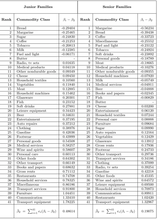
However, instead of tabulating 41 budget shares by discrete income (to-tal expenditure) intervals, the entire sample of the respective Junior and Senior families are now used toestimatethe CDESparameters, cf.(75), with herebutter (j = 2) as referencecommodtiy. The estimated parameters, ranked according to size for both life-cycle groupes, are shown in Table 2. We have given the parameter estimates without indicating the standard errors (or t-values) in Ta-ble 2; they are availlaTa-ble in Jensen (1980, p.283-85), but here omitted as such standard deviations carry little weight as economic-statistical significance indi-cators, on groundes explained by Wold (1952, p. 260). Statistically, estimates that are closer to zero (middle of Table 2) are less significant than large negative (positive) parameter estimates at the end of the rankings. Economically, the range of the reaction parameters (βi), (13), place many item values meaningful

(24)

Table 1A. Budget Shares of Social Strata : Saxony 1857.

Proportions of the Expenditure of the Family of-Items of Expenditure

Workman with an Workman with an Workman with an yearly income of yearly income of yearly income of

45 - 60£ _{90 - 120}£ _{150 - 200}£

1 Food (beverage, tobacco, taverns) 62.0 55.0 50.0

2 Clothing (footwear, jewellery) 16.0 18.0 18.0

3 Lodging (rent, utensils, furniture) 12.0 12.0 12.0

4 Light and Fuel (wood,coal, gas,oil) 5.0 5.0 5.0

5 Education (culture, church) 2.0 3.5 5.5

6 Public Protection (taxes) 1.0 2.0 3.0

7 Care of Health (medical, pharma) 1.0 2.0 3.0

8 Personal Services 1.0 2.5 3.5

Totals 100.0 100.0 100.0

Source: Marshall (1920, p. 115); Engel (1857, 1895, p. 30).

Table 1B. Budget Shares of Social Strata : Sweden 1913-1933.

Industrial worker families Middle class families Item group

1913 1923 1933 1923 1933

1 Nourishment 50.4 47.8 40.0 31.5 28.5

2 Clothing 14.2 16.0 14.6 14.5 14.4

3 Fuel, Light, Laundry 6.4 6.5 6.1 6.2 6.0

4 Housing 13.3 11.6 16.9 13.5 18.2

5 Furniture (furnishings) 4.7 4.8 5.2 7.1 6.4

6 Personal Services (domestic) 1.0 0.5 0.4 4.2 3.3

7 Hygiene (medical care) 1.8 2.3 3.2 2.8 3.3

8 Education (culture, travel) 5.0 6.2 7.0 9.2 9.7

9 Other Expenditures 3.1 4.2 6.6 11.0 10.2

All expenditures 100.0 100.0 100.0 100.0 100.0

Source: Wold (1952, p. 20); Recalculation with all expenditures =C.

Table 1C. Budget Shares : Families in the U.S.A. 1918-19

Item group 100ei 1 Food 38.9 2 Clothing 16.2 3 Fuel, Light 5.4 4 Rent 13.6 5 Furnishings 5.0 6 Miscellaneous 20.9 Total 100.0 Source: Leser (1941, p. 53).

(25)

In judging the validity and reliability of the parameter estimates, a main crite-rion will the overall consistency obtained for the different budget items within and between social strata, and proper comparisons and checks with specific evi-dence from other sources and periods. Looking at thepoint estimatesin Table 2 for the two family types, a main feature of the results is that astable hierarchy exists between the item groupes in theirpreference and demand sensitivity, as was evident in budget shares of Table 1 discussed above.

The CDESexpenditure(“income”)elasticitiesof the 41 consumer goods and services, satisfying Engel aggregation, are shown in Table 3. The methods and formulas employed in calculating the elasticities in Table 3 from Table 1 and Table 2 have been explained above in section 3. Hence with butter (j= 2) as reference commodity of the estimates in Table 2 and (31), we get for butter

E(Y2, C) = 1− 41 X i=1 ei(βi−β2) = 1−β¯2= 1−0.48614 = 0.51386 (80) E(Y2, C) = 1−β¯2= 1−0.19075 = 0.80925 (81)

of Junior/ Senior families - evaluated at, respectively, (C= 42557, C= 40831). All the other elasticities in Table 3 are then calculated from (35), (80),(81), and Table 2 as, respectively,

E(Yi, C) =E(Y2, C) +βi−β2= 0.51386 +βi−β2 (82) E(Yi, C) = 0.80925 +βi−β2 (83)

The main feature of the results obtained in Table 3 (with the same ranking as in Table 2) is the overallsimilaritythat subsists between the commodity classes in their expenditure (income) sensitivity for the two life-cycle groupes (apart from some obvious differences already mentioned, cf. Table 1). Since the sample average of C was higher for the Junior groupe, the item elasticities E(Yi, C)

should ceteris caribus be smaller for the Junior families, cf. (24), (31), and their size in Table 3 comply with such tendency.

Several food items are among the necessities with the lowets elasticities, al-though fancy food also exists among the luxuries for both groupes (rank 31, 35). Clothing, footwear, and goods and services associated with dwelling operations have elasticities around one. Housing, furniture, and cars are the high elastic-ity goods for Juniors, and latter good also tops the list for the Senior families. The CDES elasticities in Table 3 display a pattern and numerical values that conform with the general picture of abundant empirical demand studies.

(26)

Table 2 : Ranking of the Reaction Parameter Estimates: (βi−β2)

Junior Families Senior Families

Rank Commodity Class βi−β2 Rank Commodity Class βi−β2

1 Bread -0.29404 1 Margarine -0.56234

2 Margarine -0.25465 2 Bread -0.39438

3 Sugar -0.24830 3 Coffee -0.33723

4 Coffee -0.21253 4 Miscellaneous -0.25552

5 Tobacco -0.20813 5 Fuel and light -0.23122

6 Milk -0.12385 6 Tobacco -0.24924

7 Fuel and light -0.06171 7 Soft drinks -0.23892

8 Butter - 8 Personal goods -0.18789

9 Radio, tv sets 0.01635 9 Meat -0.18665

10 Medical products 0.04118 10 Medical products -0.10276

11 Other nondurable goods 0.09349 11 Other nondurable goods -0.09355

12 Cheese 0.09450 12 Household machines -0.07920

13 Household textiles 0.10560 13 Milk -0.05749

14 Vegetables 0.11840 14 Medical services -0.04911

15 Meat 0.12885 15 Beer -0.04888

16 Household machines 0.15462 16 Books and papers -0.02345

17 Glassware 0.20301 17 Fish -0.00829

18 Fish 0.23152 18 Butter

-19 Soft drinks 0.27881 19 Cheese 0.03200

20 Leisure equipment 0.34423 20 Entertainment 0.06120

21 Beer 0.34631 21 Household textiles 0.07244

22 Entertainment 0.37195 22 Personal care 0.08888

23 Auto repairs 0.37212 23 Furniture 0.09684

24 Clothing 0.38976 24 Sugar 0.09990

25 Gasoline 0.42036 25 Auto repairs 0.12164

26 Footwear 0.43999 26 Vegetables 0.12429

27 Personal goods 0.54508 27 Glassware 0.13912

28 Medical services 0.58257 28 Gross rents 0.17936

29 Wine and spirits 0.58607 29 Footwear 0.24733

30 Personal care 0.60113 30 Other transport 0.29736

31 Other foods 0.64302 31 Transport services 0.34186

32 Other transport 0.66149 32 Clothing 0.37099

33 Books and papers 0.68632 33 Radio, tv sets 0.39254

34 Gross rents 0.71112 34 Gasoline 0.42218

35 Restaurants 0.74708 35 Other foods 0.45335

36 Household services 0.78325 36 Wine and spirits 0.64572

37 Miscellaneous 0.86186 37 Leisure equipment 0.69500

38 Transport services 0.91800 38 Household services 0.70973

39 Furniture 1.04451 39 Communication 0.89911

40 Communication 1.33410 40 Restaurants 1.02420

41 Transport equipment 1.78225 41 Transport equipment 1.32967

¯

(27)

Table 3: Estimates of Expenditure (“Income”) Elasticities

Goods and Services :

E

(

Y

i

, C

) =

E

(

P

i

Y

i

, C

)

Rank Commodity Class E(Yi, C) Rank Commodity Class E(Yi, C)

1 Bread 0.21982 1 Margarine 0.24691

2 Margarine 0.25921 2 Bread 0.41487

3 Sugar 0.26556 3 Coffee 0.47202

4 Coffee 0.30133 4 Miscellaneous 0.55373

5 Tobacco 0.30573 5 Fuel and light 0.57803

6 Milk 0.39001 6 Tobacco 0.56001

7 Fuel and light 0.45215 7 Soft drinks 0.57033

8 Butter 0.51386 8 Personal goods 0.62136

9 Radio, tv sets 0.53021 9 Meat 0.62260

10 Medical products 0.55504 10 Medical products 0.70649

11 Non-durable goods 0.60735 11 Non-durable goods 0.71570

12 Cheese 0.60836 12 Household machines 0.73005

13 Household textiles 0.61946 13 Milk 0.75176

14 Vegetables 0.63226 14 Medical services 0.76014

15 Meat 0.64271 15 Beer 0.76037

16 Household machines 0.66848 16 Books and papers 0.78580

17 Glassware 0.71687 17 Fish 0.80096

18 Fish 0.74538 18 Butter 0.80925

19 Soft drinks 0.79267 19 Cheese 0.84125

20 Leisure equipment 0.85809 20 Entertainment 0.87045

21 Beer 0.86017 21 Household textiles 0.88169

22 Entertainment 0.88581 22 Personal care 0.89813

23 Auto repairs 0.88598 23 Furniture 0.90609

24 Clothing 0.90362 24 Sugar 0.90915

33 Books and papers 1.20018 33 Radio,, tv sets 1.20179

41 Transport equipment 2.29611 41 Transport equipment 2.13892

P41

i=1eiE(Yi, C) 1.00000

P41

(28)

7. Reaction Parameters, Price and Substitution Elasticities

The information about the estimated differences (βi−β2) in Table 2 were

suffi-cient for calculating income elasticities of CDES demand, (16), (82); adding an arbitrary constant to all theβi- parameters would not change the elasticity with

the respect toC in (16) - whereas any particular price elasticity would clearly be affected by such additive constant in everyβi. Thus CDES price elasticities

cannot be calculated from Table 2; moreover, the ’reaction parameters’(βi)

can-not be fully recovered from just family budget surveys (expenditure data). But they are as ’invariances’ (basic parameters) - in contrast to continuosly changing income and price elasticities - the ultimate empirical objective to obtain for the CDES indirect utility function and demand system, (7), (16).

As mentioned at the end of section 5,extranousinformation (literature sur-veys, benchmark observations, calibration procedures) on any single price elas-ticty will in combination with Tabele 2 allow full identification and estimation of all the parameters, (βi). Our parameter calibrations will be based on the price

elasticity of butter that is a well-defined homogenoues good and a classic article of many demand studies - convenient also as being our reference commodity.

Hence by (16), the reaction parameter for butter will becalibratedas

β2= [E(Y2, P2)−1]/(1−e2) (84)

Market statistics in the form of time series are often seen as the principal ma-terial for the estimation of direct price and cross price elasticties. However, our elasticity and parameter in (84) do not refer to total butter market demand, but instead to butter demand elasticities segmented to our life-cycle groups. Accordingly information from specialized demand studies are called for ; such food demand analyses are available, since our life cycle categories have been standard for a long time in many countries.

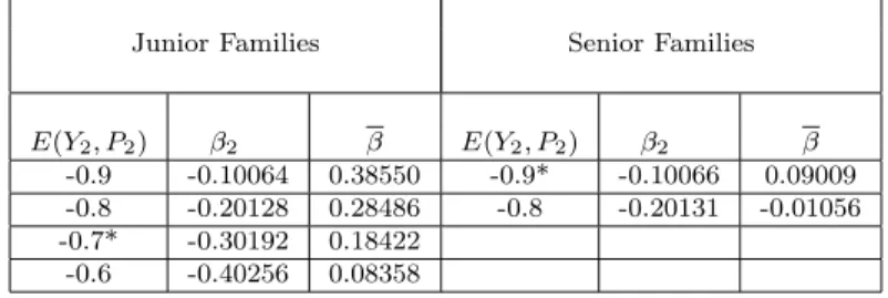
Calculations ofβ2 by (84) - for different butter price elasticities and withe2

from Table 1 - are collected in Table 4a. The starred price elastities appear as the most plausible ones for several reasons. They are partly in line with butter elasticities seen for our family types in Wold & Juren (1952, p. 266-69, 285-88), conform properly with the income elasticities, (80),(81), and fit in appropriately with the wider implications of the correspondingβ2(andβ) values upon all the

other price elasticities, as explained below.

Table 4a. Reaction Parameter β2, β, and E(Y2,P2).

E(Y2, P2) β2 β E(Y2, P2) β2 β

-0.9 -0.10064 0.38550 -0.9* -0.10066 0.09009

-0.8 -0.20128 0.28486 -0.8 -0.20131 -0.01056

-0.7* -0.30192 0.18422 -0.6 -0.40256 0.08358

(29)

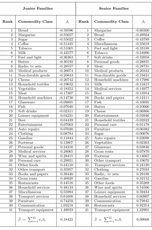
Table 4: Ranking and Size of Reaction Parameter Estimates: (βi)

Rank Commodity Class βi Rank Commodity Class βi

1 Bread -0.59596 1 Margarine -0.66300

2 Margarine -0.55657 2 Bread -0.49504

3 Sugar -0.55022 3 Coffee -0.43789

4 Coffee -0.51445 4 Miscellaneous -0.35618

5 Tobacco -0.51005 5 Fuel and light -0.33188

6 Milk -0.42577 6 Tobacco -0.34990

7 Fuel and light -0.36363 7 Soft drinks -0.33958

8 Butter -0.30192 8 Personal goods -0.28855

9 Radio, tv sets -0.28557 9 Meat -0.28731

10 Medical products -0.26074 10 Medical products -0.20342

11 Non-durable goods -0.20843 11 Non-durable goods -0.19421

12 Cheese -0.20742 12 Household machines -0.17986

13 Household textiles -0.19632 13 Milk -0.15815

14 Vegetables -0.18352 14 Medical services -0.14977

15 Meat -0.17307 15 Beer -0.14954

16 Household machines -0.14730 16 Books and papers -0.12411

17 Glassware -0.09891 17 Fish -0.10895

18 Fish -0.07040 18 Butter -0.10066

19 Soft drinks -0.02311 19 Cheese -0.06866

20 Leisure equipment 0.04231 20 Entertainment -0.03946

21 Beer 0.04439 21 Household textiles -0.02822

22 Entertainment 0.07003 22 Personal care -0.01178

23 Auto repairs 0.07020 23 Furniture -0.00382

24 Clothing 0.08784 24 Sugar -0.00076

33 Books and papers 0.38440 33 Radio,, tv sets 0.29188

41 Transport equipment 1.48033 41 Transport equipment 1.22901 ¯

β = P41

i=1eiβi 0.18422 β¯ =

P41

(30)

This selection of (β2) from Table 4a together with Table 2 finally give the

sizesfor the complete set of reaction parameters, listed in Table 4. Meaningful interpretation and comparison between the numbers for junior/senior families were not possible (despite correct ranking) in Table 2, asβ2was unknown and

might be widely different for such life-cycle groupes. Overall the numbers in Table 4 now look more similar (min, range) for the two family types, although natural differences in their preferences still exist. As to Junior families, the six items at the top of the table are more ’urgent necessities’ than those of the Seniors. On the other hand, the average urgency (rigidity) level (β) is somewhat lower for the Juniors, respectively. The location and different sizes of item specific reaction parameters (βi) will affect the pattern of price elasticities

of demand for the two family types.

The Marshallian & Slutsky price elasticities (own, cross), and the Allen substitution elasticities - calculated from Table 4 and Table 1 according to their parametric formulas given in section 3 - are together with income elasticities exhibited for the respective life-cycle groupes in Tables 5A-5B, Tables 6A-6B. For ease of discussion and numerical accuracy evaluations, the item budget shares (100ei) are included in these tables - as are the exact consistency checks

by the Engel and Cournot aggregations and homogeneity restrictions.

As seen from the listedown-(direct) price elasticitiesof commodities in Table 5A and Table 6A, the Marshall and Slutsky own-price elaticities have nearly the same size (differing in most cases only on second decimals). Evidently, the“income effect”of own-price changes upon Marshallian price elastcities are verysmall, when a large number of commodities (and hence individually small budget shares) are involved, cf. (46). Since no inferior goods were actually observed (estimated) for neither Junior nor Senior families in Table 3, all the Marshallian price elasticties in Tables 5A and Table 6A are abslolutely larger than the corresponding Slutsky (“compensated”) elasticity.

We see for CDES income and price elasticities, Tables 5A, 6A, cf. (30), (39),

E(Yi, C) +E(Yi, Pi) = −β¯+βiei; β¯= 0.18422, β¯= 0.09009 (85)

and for the differences of price elasticities, cf. (39),

E(Yi, Pi)−E(Yj, Pj) = −(βi−βj) +βiei−βjej (86)

Compared to (35), the sum/differences in (85), (86) are not exactly constant, but nearly so, when large number of items are involved (smallei). On this CDES

background and and its elasticity numbers, we next search for some clues about the magnitudes and general numerical pattern among various price elasticities. Whereas Engel aggregation implies that some income elasticties are to be larger and some other must be smaller than 1, no such rule are implied by the budget constraint for the own-price elastcities. They can all exceed one (elastic) or all be inelastic without violating any conditions imposed by consumer demand theory or budget constraints. The Cournot aggregation implied by the budget constraint, however, does give some indication about the mutual relationships