DEPARTMENT OF ECONOMICS
UNIVERSITY OF MILAN - BICOCCA
WORKING PAPER SERIES
Sticky Wages and Rule of Thumb Consumers
Andrea Colciago
No. 98 – September 2006
Dipartimento di Economia Politica
Università degli Studi di Milano - Bicocca
Sticky wages and rule of thumb consumers.
Andrea Colciago
∗University of Milano-Bicocca
November 2, 2006
Abstract
I introduce sticky wages in the model with credit constrained or “rule of thumb” consumers advanced by Galì, Valles and Lopez Salido (2005). I show that wage stickiness i) restores, in contrast with the results in Bilbiie (2005), the Taylor Principle as a necessary condition for equilib-rium determinacy; ii) implies that a a rise in consumption in response to an unexpected rise in government spending is not a robust feature of the model. In particular, consumption increses just when the elasticity of marginal disutility of labor supply is low. Results are robust to most of Taylor-type monetary rules used in the literature, including one which responds to wage inflation.
JEL classification: E32, E62.
Keywords: Sticky Prices, Sticky Wages, Rule of Thumb Consumers.
∗Address: Department of Political Economy, University of Milano-Bicocca, piazza
dell’Ateneo Nuovo 1, 20126, Milano, Italy. Tel: +39 02 6448 3065, e-mail: an-drea.colciago@unimib.it.
1
Introduction
Recent evidence on U.S. data, provided amongst others by Blanchard and Per-otti (2002) and Galì, Valles and Lopez-Salido (2005, GVL henceforth) seems to suggest that private consumption does not decrease after a government purchase shock. Nevertheless, most of dynamic macroeconomic models predicts that a rise in government purchases will have a contractionary effect on consumption. Although the evidence is controversial, the literature has identified this sharp contrast between the implications of the theory on one hand, and empirical re-sults on the other, as a puzzle. Much effort has been devoted to the construction of theoretical models which could solve the puzzle.
One candidate solution, which has received considerable interest, is that ad-vanced by GVL. The interest is partly due to the simplicity of their approach. They consider a sticky prices New Keynesian economy, where part of the con-sumers are standard optimizing agents who trade a consumption good on contin-gent markets and are endowed with a common initial stock of physical capital. The rest of the population is constituted by non ricardian or “rule of thumb” households who consume in each period their labor income. GVL show that this framework allows to obtain a positive response of aggregate consumption to a government spending shock.
Three ingredients are necessary to generate the crowding-in of aggregate consumption. Thefirst one is a large enough share of non ricardian consumers, the second is a substantial degree of price stickiness and the third one is that the increase in public expenditure is partly debtfinanced.
Notice that the crowding-in of consumption is obtained via a strong increase in the real wage, which has the effect of driving up consumption of non ricardian households.
Campbell and Mankiw (1989)find evidence of rule of thumb behavior. Using U.S. aggregate post-war data, they estimate that about half of total income goes to non ricardian consumers. More recently Muscatelliet al (2004), using U.S. quarterly data over the period 1970-2001, document that about 37% of consumers are rule of thumb.
The evidence relative to the response of real wages to a fiscal shock is as controversial as that on consumption. While Fisheret al (2004)find a negative effect of fiscal shocks on real wages, Blanchard and Perotti (2002) and Fatas and Mihov (2002)find a positive, but limited, response.
In any case, none of these works allows to rely on a rise in real wage to explain the crowding-in effect.
Turning to the role of monetary policy within the GVL’s model, the most significant result is provided by Bilbiie (2005). He points out that the presence of rule of thumb consumers may change the determinacy condition that the literature has labeled theTaylor Principle. Under a reasonable parametrization of the share of non ricardian consumers, no capital accumulation and a walrasian labor market, he shows that a passive rule is necessary for determinacy.
A natural extension of the GVL model calls for the introduction of some form of frictions in the wage setting process.
The model economy I describe differs from that in GVL for what concerns the structure of the labor market and the wage setting arrangements. Beside considering imperfectly competitive markets, we assume that wages are set in a staggered fashion according to the Calvo mechanism considered in Ercegat al
(2000) or Schmitt-Grohe and Uribe (2004a).
Keyfindings are that nominal wage stickiness i) restores the Taylor Principle as a necessary condition for equilibrium determinacy; ii) alters the impulse response function of the model economy after a government spending shock.
With respect to i), I show that, when the degree of wage stickiness is set according to the available estimates, the Taylor Principle returns a necessary condition for uniqueness.
This stands in sharp contrast with the results in Bilbiie (2005). A passive rule may lead to uniqueness of the REE just when wages are moderately sticky (average duration of 2-3 quarters) and the share of non ricardian consumers is well above the estimates. For these reasons I regard this case as of minor empirical interest. Since wage stickiness is an uncontroversial empirical fact, the result should be of importance for the central banker concerned with avoiding sunspotfluctuations.
With respect to ii), I establish that the crowding-in of consumption is no longer a robust feature of the model. Wage stickiness dampens real wagefl uctu-ations associated to variation in real activity induced by government spending shocks. This limits the large rise in consumption of non ricardian consumers which is, instead, registered in a model with flexible wages. For empirically plausible values of the parameters, the crowding-in of consumption vanishes.
A government purchase shock generates a positive response of aggregate consumption when the agents suffer a low marginal cost of supplying labor in terms of utility. In this case, the increase in hours worked associated with the spending shock is enough to boost consumption of non ricardian agents. As in GVL if the share of non ricardian consumers is large enough, aggregate consumption will experience a positive variation.
Results are robust to the different kinds of Taylor rules proposed in the literature, including one which reacts to wage inflation.
Other proposals, beside that of GVL, have been advanced to solve the Gov-ernment spending puzzle. Linneman (2006) suggests that the puzzle can be amended in a frictionless business cycle model by resorting to non-separable preferences. The employment-consumption complementarity generated by this form of preferences favours a positive response of consumption to an innova-tion in government spending. However, as pointed out by Bilbiie (2006), the restrictions on preferences imposed by Linnemann (2006) are such that labor supply schedule is downward sloping. Bilbiie (2006) goes on showing that the conditions under which non-separability solves the Government spending puzzle imply that the consumption good is inferior.
Linneman and Schabert (2006) describe a new Keynesian model where gov-ernment expenditure contributes to aggregate production. In this case inno-vations in Government spending lead to a rise in private consumption when the government share in consumption is not too large. Nevertheless, assuming
that Government purchases enter into the production function is a remarkable departure from standard business cycle theory.
In a nutshell, the message of the paper is the following. The model with rule of thumb consumers may not lead to a positive response of aggregate consump-tion to a government spending shock when wages are sticky. Further, when a share of agents is constrained to consume out of current income, the design of monetary policy cannot neglect the details of the wage setting process.
1.1
Firms
In each period t afinal good Yt is produced by a perfectly competitive firm,
combining a continuum of intermediate inputsYt(z), according to the following
standardCES production function:
Yt= µZ 1 0 Yt(z) ϑp−1 ϑp dz ¶ ϑp ϑp−1 with θp>1 (1)
The producer of thefinal good takes prices as given and chooses the quantities of intermediate goods by maximizing its profits. This leads to the demand of intermediate goodz and to the price of the final good which are respectively
Yt(z) = ³Pt(z) Pt ´−θp Yt ; Pt= hR1 0 Pt(z) 1−ϑpdz i 1 1−ϑp
Intermediate inputsYt(z)are produced by a continuum of size one of
mo-nopolisticfirms which share the following technology:
Yt(z) =Kt−1(z)αLt(z)1−α
where 0 < α < 1 is the share of income which goes to capital in the long run, Kt−1(z) is the time t capital service hired by firm z, whileLt(z) is the
timet quantity of the labor input used for production. The latter is defined as
Lt= µR 1 0 L jθwθw−1 t dj ¶ θw θw−1
with θw >1. Firm’s z demand for labor typej and
the aggregate wage index are respectively
Ljt(z) =³Wtj Wt ´−θw Lt(z) ; Wt= µR 1 0 ³ Wtj´1−θwdj ¶1/(1−θw)
The nominal marginal cost is given by
M Ct= µ 1 α ¶αµ 1 (1−α) ¶1−α Wt1−α¡Rkt¢α
Price setting. I assume firms set prices according to the mechanism spelled out in Calvo (1983). Firms in each period have a chance1−ξp to reoptimize their price. A price setter z takes into account that the choice of its time t nominal price, Pet, might affect not only current but also future profits. The
associatedfirst order condition is:
Et ∞ X s=0 ¡ βξp¢sνt+sPtθ+sYt+s h e Pt−µpPt+sM Ct+s i = 0 (2)
which can be given the usual interpretation.1 Notice that µp = θp
θp−1
repre-sents the markup over the price which would prevail in the absence of nominal rigidities.
1.2
Labor market
The description of the labor market follows Colciagoet al (2006). I assume a continuum of differentiated labor inputs indexed by j. Wage-setting decisions are taken by a continuum of unions. More precisely union j monopolistically supplies labor inputj on labor marketj. Unionj sets the nominal wage,Wtj, in order to maximize a weighted average of both agents’ utilities, taking as given
firms’ demand for its labor service. 2 As in Schmitt-Grohé and Uribe (2004a), agentisupplies all labor inputs. Further, following GVL, we assume that agents are distributed uniformly across unions.3 Firms allocate labor demand on the
basis of the relative wage, without distinguishing on the basis of household types. This implies that once the union hasfixed the nominal wage, aggregate demand of labor typej is spreaded uniformly between all households. In other words, individual levels of employment and labor income are the same across households. The latter is given byLd
t R1 0 W j t ³Wj t Wt ´−θw dj =WtLdt, whereLdt is
aggregate labor demand.4 1ν
tis the value of an additional dollar for a ricardian household. As it will be clear below,
is the lagrange multiplier on ricardian househols nominalflow budget constraint.
2The union objective function is descrived below as, at this stage, we just provide a
de-scription of the labor market structure.
3This implies that a shareλof the associates of each union is composed by non ricardian
agents.
4Erceget al (2000), assume, as in most of the literature on sticky wages, that each agent
is the monopolistic supplier of a single labor input. In this case, assuming that agents are spreaded uniformly across unions allows to rule out differences in income between households providing the same labor input (no matter whether they are ricardian or not), but it does not allow to rule out difference in labor income between non ricardian agents that provide different labor inputs. This would amount to have an economy populated by an infinity of different individuals, since non ricardian agents cannot share the risk associated to labor in-comefluctuations. Although this framework would be of interest, it would imply a tractability problem.
1.3
Households
There is a continuum of households on the interval[0,1]. As in GVL,households in the interval[0, λ]cannot accessfinancial markets and do not have an initial capital endowment. The behavior of these agents is characterized by a simple rule of thumb: they consume their available income in each period. The rest of the households on the interval(λ,1], instead, is composed by standard ricardian households who have access to the market for physical capital and to a full set of state contingent securities. I assume that Ricardian households hold a common initial capital endowment. The period utility function is common across households and it has the following separable form
Ut=u(Ct(i))−v(Lt(i))
whereCt(i)is agenti’s consumption andLt(i)are labor hours. It follows that
the total number of hours allocated to the different labor markets must satisfy the time resource constraintLt(i) =R01Ljt(i)dj
Ricardian households. Ricardian Households’ timet nominal flow budget reads as
Pt(Cto+Ito) + (1 +Rt)−1Bto+EtΛt,t+1Xt+1 (3)
≤ Xt+WtLdt +RktKto−1+Bto−1+PtDot−PtTto
we assume that ricardian agents have access to a full set of state contingent assets. More precisely, in each time periodt, consumers can purchase any de-sired state-contingent nominal paymentXt+1 in period t+1 at the dollar cost
EtΛt,t+1Xt+1. Λt,t+1 denotes a stochastic discount factor between periodt+ 1
andt. WtLdt denotes labor income andRktKto−1is capital income obtained from
renting the capital stock tofirms at the nominal rental rate Rk
t. PtDot are
div-idends due from the ownership offirms, whileBo
t is the quantity of nominally
riskless bonds purchased in periodt at the price(1 +Rt)−1and paying one unit
of the consumption numeraire in periodt+1. PtTtorepresent nominal lump sum
taxes. As in GVL, the household’s stock of physical capital evolves according to: Kto= (1−δ)Kto−1+σ µ Ito Ko t−1 ¶ Kto−1 (4) whereδdenotes the physical rate of depreciation. Capital adjustment costs are introduced through the term σ³ Iot
Ko t−1
´
Kto−1, which determines the change in the capital stock induced by investment spending Io
t. The functionσ satisfies
the following properties:
σ0(·)>0,σ00(·)≥0,σ0(δ) = 1,σ(δ) =δ
Thus, adjustment costs are proportional to the rate of investment per unit of installed capital. Ricardian households face the, usual, problem of maximizing
the expected discounted sum of istantaneous utility subject to constraints(3)
and (4). νt and Qt denote the Lagrange multipliers on the first and on the
second constraint respectively. β = 1
1+ρ is the discount factor, whereρ is the
time preference rate. Thefirst order conditions with respect toCo
t,Ito,Bto,Kto, Xt+1are uc(Cto) =νtPt (5) 1 φ0³ Iot Ko t−1 ´ =qt (6) 1 (1 +Rt) =βEt νt+1 νt (7) Qt=Et ½ Λt,t+1 · Rkt+1+Qt+1 µ (1−δ)−φ0 µIo t+1 Ko t ¶Io t+1 Ko t +φ µIo t+1 Ko t ¶¶¸¾ (8) Λt,t+1=β νt+1 νt (9) where qt = QPtt is the real shadow value of installed capital, i.e. Tobin’s Q.
Substituting (5) into (9) we obtain the definition of the stochastic discount factor Λt,t+1=β uc ¡ Co t+1 ¢ Pt+1 Pt uc(Cto)
while combining(9)and(7)we recover the following arbitrage condition on the asset market
EtΛt,t+1= (1 +Rt)−1
Non ricardian households. Non ricardian households maximize period util-ity subject to the constraint that they have to consume available income in each period, that is
PtCtrt =WtLdt−PtTtrt (10)
As in GVL I let lump sum taxes (transfers) paid (received) by non ricardian households differ by those paid by ricardian.
1.4
Wage Setting
Nominal wage rigidities are modeled according to the Calvo mechanism used for price setting. In each period a union faces a constant probability1−ξw of
being able to reoptimize the nominal wage. I follow GVL, and assume that the nominal wage newly reset at t,fWt, is chosen to maximize a weighted average of
agents’ lifetime utilities. The union objective function is
Et ∞ X s=0 (ξwβ)s £ (1−λ)u¡cot+s¢+λu¡crtt+s¢¤+v Ldt+s 1 Z 0 à Wtj+s Wt+s !−θw dj
The FOC with respect tofWtis Et ∞ X s=0 (βλw)t+sΦt,t+s (· λ 1 M RSrt t+s + (1−λ) 1 M RSo t+s ¸ fWt Pt+s − µw ) = 0 (11) where Φt,t+s = vL(Lt+s(i))Ltd+sWtθw and µw = (θwθw−1) is the, constant,
wage mark-up in the case of wage flexibility. M RStrt+s and M RSot+s are the
marginal rates of substitution between labor and consumption of non ricardian and ricardian agents respectively. Notice that when wages are flexible (11)
becomes Wt Pt =µw · λ 1 M RSrt t + (1−λ) 1 M RSo t ¸−1 (12) which is identical to the wage setting equation in GVL.
1.5
Government
The Government nominalflow budget constraint is
PtTt+ (1 +Rt)−1Bt=Bt−1+PtGt (13)
wherePtGt is nominal government expenditure on thefinal good. As in GVL
we assume afiscal rule of the form
tt=φbbt−1+φggt (14) wherett= TtY−T,gt=GtY−G andbt= Bt Pt− Bt−1 Pt−1 Y . gtis assumed to follow afirst
order autoregressive process
gt=ρggt−1+εgt (15)
where0≤ρg≤1andεgt is a normally distributed zero-mean random shock to government spending.5
1.6
Monetary Policy
An interest rate-setting rule is required for the dynamic of the model to be fully specified. I focus on the rule analyzed by GVL which features the central bank setting the nominal interest rate as a function of current inflation according to the following log-linear rule
rt=τππt (16)
5A sufficient condition for non explosive debt dynamics is
(1 +ρ) (1−φb)<1
which is satisfied if
φb>
ρ
1 +ρ I assume this condition is satisfied throughout.
where rt = log(1+1+Rρt) and πt = logPPtt
−1. In standard sticky price models
with no endogenous investment, as in Woodford (2003) or Galì (2002), rule
(16)ensures local uniqueness of a rational expectation equilibrium (REE) if it satisfies the Taylor Principle, i.e. ifτπ>1.
1.7
Aggregation
We denote aggregate consumption, lump sum taxes, capital, investment and bonds withCt,Tt, Kt,Itand Btrespectively. These are defined as
Ct=λCtrt+ (1−λ)Cto; It= (1−λ)Ito;
Kt= (1−λ)Kto;
Tt=λTtrt+ (1−λ)Tto; . Bt= (1−λ)Bto
1.8
Market Clearing
The market clearing conditions in the goods market and in the labor market imply Yt=Ct+Gt+It; Yts(z) =Ytd(z) = ³ Pt(z) Pt ´−θp Yt; ∀z Lt=Ldt; ³ Ljt´ s =³Ljt´ d =³W j t Wt ´−θw Lt; ∀j whereLd t = R1 0 Lt(z)dz and ³ Ljt´d =R01Ljt(z)dz.
1.9
Steady State
As in GVL, we assume that steady state lump sum taxes are such that steady state consumption levels are equalized across agents. Firmi’scost minimization implies W P = (1−α) µp YL rk =µαpYK where K Y = α µp(ρ+δ)
Since the ratio GY = γg is, by assumption, exogenous, we can determine the steady state share of consumption on output,γc, as follows
γc= 1− δα
µp(ρ+δ)−γg
which, as noticed by GVL, is independent ofλ. In what follows it will prove useful to know W P L C, which equals W P L C = (1−α) µp Y L L C = (1−α) µpγ c
2
The Log-linearized model.
To make our results readily comparable to those in GVL we assume the same period utility function considered in their work:
u(Ct) = logCt ; v(Lt) =L
1+φ t
1+φ
which feature a unit intertemporal elasticity of substitution in consumption and a constant elasticity of the marginal disutility of laborvLL=φ.6 In what
follows lower case letters denote log-deviations from the steady state values. The log-deviation of the real wage, denoted bywt, constitutes the only exception to
this rule. The conditions which define the log-linear approximation to equations of the model are derived in GVL and I report them in the appendix. I provide, instead, a detailed derivation of the wage inflation curve and of the real wage schedule.
2.1
Wage in
fl
ation, the real wage schedule and the e
ff
ect
of economic activity on the real wage.
In the case of identical steady state consumption levels, agents have a common steady state marginal rate of substitution between labor and consumption. This implies that equation(11)can be given the following log-linear approximation
Et ∞ X s=0 (βξw)t+s£wt+s−mrsAt+s ¤ = 0 wheremrsA
t =λmrsrtt +(1−λ)mrsot is a weighted average of the log-deviations
between the marginal rates of substitution of the two agents. In what follows we will refer tomrsA
t as to the average marginal rate of substitution. Given the
selected functional forms, the (log)wage optimally chosen at timet is defined as
logWft= logµw+ (1−βξw)Et
∞
X
s=0
(βξw)t+s{logPt+s+ logCt+φlogLt}
Combining the latter with the following, standard, log-linear approximation of the wage index
logWt= (1−ξw) logWft+ξwlogWt−1
we obtain the desired wage inflation curve
πwt =βEtπtw+1−κwµwt (17)
whereκw= (1−βξw)(1ξ −ξw)
w and
µwt = (logWt−logPt)−(logµw+ logCt+φlogLt).
6The selected period utility belong to the King-Plosser-Rebelo class and leads to consant
is the wage mark-up that union impose over the average marginal rate of sub-stitution.7 Due to the assumption that unions maximize a weighted average of
agents’ utilities, the wage inflation curve has a standard form. Equation (17)
allows to obtain the log-deviation of timet real wage, which plays a prominent role in the determination of non ricardian agents consumption, as follows
wt=Γ[wt−1+β(Etwt+1+Etπt+1)−πt+κw(φlt+ct)] (18)
where Γ= ξw
(1+βξ2
w). Today’s average real wage is a function of its lagged and
expected value, expected and current inflation. The termφlt+ctrepresents the
average real wage that would prevail in the case of wageflexibility. Γdetermines both the degree of forward and backward lookingness.8 Substituting(27)into
(18)we get:
wt=Γwt−1+Γβ(Etwt+1+Etπt+1) +Ψyt−Ψαkt−1+Γκwct−Γπt (19)
where Ψ=Γ κw
(1−α)φdetermines the effect on the real wage due to changes in
the level of real activity. Comparative statics. ∂ξ∂Γ
w >0: a longer average duration of wage contracts
does not have a clear cut effect on real wage inertia. Asξwgets larger both forward and backward lookingness increase. ∂Ψ
∂φ >0: the more elastic is
the marginal disutility of labor, i.e. the higher is φ, the higher is the sensitivity of wages to an increase in economic activity. ∂ξ∂Ψ
w < 0: the
higher is average duration of wage contracts, i.e. the higher is ξw, the lower is the sensitivity of wages to an increase in economic activity. Intuition goes as follows. A higher ξw implies that the nominal wage will be newly reset on a limited number of labor markets, thus the previous period average wage has a stronger influence on today’s. At the same time those unions which optimally reset their wage will attach a higher weight on expected future variables. The parameter Ψ determines the size of the variation in real wage associated with a given variation in real economic activity. This is jointly determined by the probability that wages cannot be changed in a given period,
ξw, and the elasticity of the marginal disutility of labor,φ.
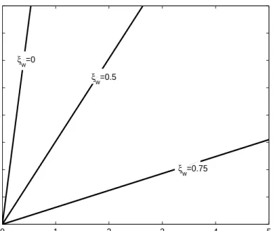
Woodford and Rotemberg (1997) report evidence suggesting that the output elasticity of real wage is in a neighborhood of 0.3.
Figure 1 plotsΨas a function ofφfor alternative degrees of wage stickiness assuming the values β = 0.99 and α = 13. Empirical estimates suggest that wages have an average duration of an year (ξw= 0.75). In this case, a value of
7As pointed out by Schmitt-Grohe and Uribe (2004a), the coefficientκ
wis different form
that in Erceg et al (2000), which is the standard reference for the analysis of nominal wage stickiness.The reason is that we have assumed that agents provide all labor inputs. In the more standard case in which each individual is the monopolistic supplier of a given labor input,κw would be equal to (1−ξβξw)(1−ξw)
w(1+φθw) hence lower than in the case we consider.
Ψconsistent with the estimates in Rotemberg and Woodford (1997) is obtained by settingφclose to 5.
In a model with a frictionless labor market this would lead to an intertem-poral elasticity of substitution in labor supply equal to0.2, which is in line with the micro-evidence in Card (1991) and Pencavel (1986). Thus, I obtain a output sensitivity of real wage consistent with the estimates using empirically plausible values ofφandξw.
This is not the case under wage flexibility. When ξw = 0 equation (19)
reduces to wt= φ (1−α)yt− α (1−α)φkt−1+ct
which is the wage setting equation in GVL. In order to be consistent with the afore-mentioned evidence on the output elasticity of real wage GVL setφ
equal to 0.2. This value is, however, far from consistent with the microeco-nomic evidence on the elasticity of labor supply and from standard calibration of preferences.
3
Calibration
We calibrate the parameters of the model since the analysis of equilibrium de-terminacy and equilibrium dynamics that follow draws on numerical results. The time unit is meant to be a quarter. In the baseline parametrization we setξw= 0.75, which implies an average duration of wage contracts of one year as suggested by the estimates in Smets and Wouters (2003) and Levineet al
(2005). αand β assume the standard values of 1
3 and 0.99 respectively. Table
1 reports the output sensitivity of real wageΨas a function of φ. In column 2 I consider the baseline calibration for wage stickiness, while in column 4 I evaluateΨunder the limiting case of wageflexibility.
Table 1 shows that, under the baseline calibration for wage stickiness, set-ting φ = 4.84 allows to match the output elasticity of real wage reported by Rotemberg and Woodford (1997), thus I take this value as the baseline. How-ever, to evaluate the dependence of the model’s implications on the elasticity of the marginal disutility of labor, we consider two other values ofφbeside the baseline. The first, φ = 0.2, corresponds to the value employed by GVL, the secondφ= 1is chosen because commonly employed in the literature. The table, consistently with the discussion in the previous section, points out that when standard values are assigned toφ, theflexible wage scenario leads to extremely high output sensitivity of real wage.
Remaining parameters are displayed in table 2, and the reader can refer to the references reported in GVL for empirical evidence supporting them. How-ever, it is worth mentioning that in the baseline calibration τπ is set to 1.5.
Table 1: Output sensitivity of real wage as a function of the elasticity of labor disutility and the calvo parameter on wages.
Ψ Ψ
φ=0.2;ξw=0.75 0.011 φ=0.2;ξw=0 0.3
φ=1;ξw=0.75 0.055 φ=1; ξw=0 1. 5
φ=4.84;ξw=0.75 0.300 φ=4.84; ξw=0 7. 26
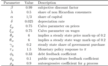
Table 2: Baseline calibration
Parameter Value Description
β 0.99 subjective discount factor
λ 0.5 share of non Ricardian consumers
α 1/3 share of capital
δ 0.025 depreciation rate
ξp 0.75 Calvo parameter on prices
ξw 0.75 Calvo parameter on wages
θp 6 implies a steady state price mark-up of 0.2
θw 6 implies a steady state wage mark-up of 0.2
γg 0.2 steady state share of government purchase
τπ 1.5 Monetary policy response toπ
φb 0.33 debt feedback coefficient
φg 0.1 public expenditure feedback coefficient
ρg 0.9 autoregressive coefficient forg process
4
Determinacy analysis
In what follows I consider the effect of wage stickiness and the share of non ricardian consumers on the determinacy properties of the REE. I initially assume that the interest rate is set according to equation(16)and then generalize results to other Taylor-type rules commonly employed in the literature.
Figure 2 depicts indeterminacy region in the parameter space (λ, τπ)under
the baseline calibration. Visual inspection of the figure leads to the following result.9
Result 1. Wage stickiness and the Taylor principle. Under the baseline parametrization, the original Taylor Principle, i.e. τπ >1, is a necessary
condition for equilibrium determinacy.
Figure 2 shows that the Taylor Principle is necessary to rule out indetermi-nate as well as unstable equilibria. In Figure 3 I address the sensitivity of the result to the degree of wage stickiness.
Panel a depicts the case of wageflexibility(ξw= 0), in panelb wages have
an average duration of 2 quarters (ξw= 0.5) while in panel c of 10 quarters
9The grid search we use to discern determinate combinations of λ and τ
π takes a step
(ξw= 0.9).
Panelsashows that for values ofλ≥0.2a passive rule leads to a determinate equilibrium. However, when the average duration of wage contracts is of two quarters (panelb), the threshold value ofλfor which a passive rule leads to a determinate equilibrium increases markedly. Panelc shows that increasing the degree of wage stickiness to values above the baseline does not alter result 1.
The analysis suggests that the results in Bilbiie (2005) are affected by the introduction of nominal wage rigidity. With an average duration of wage con-tracts of 2 quarters, which is well below the estimates we have reported, 75% of the households should be fully credit constrained for a passive rule to implement a determinate equilibrium. This is above the values suggested in the literature. Empirical evidence in Campbell and Mankiw (1989) for the U.S., and Muscatelli
et al (2003) for the Euro area, support the view that a plausible value for the share of non ricardian consumers is in a neighborhood of 0.5.
Figure 4 depicts indeterminacy region in the parameter space¡ξp, λ
¢
. Again, each panel corresponds to a different degree of wage stickiness.10 Monetary policy response to current inflation is kept at its baseline value of1.5.11 Visual
inspection of thefigure leads to result 2.
Result 2. Indeterminacy and wage stickiness. Wage stickiness affects the determinacy properties of the rational expectation equilibrium. In partic-ular, asξwincreases indeterminate regions fairly rapidly contract, decreas-ing the likelihood of sunspotsfluctuations.
Panel c considers the baseline parametrization for wage stickiness. In this case, ifλis set to 0.5, as suggested by the estimates of Campbell and Mankiw (1989), falling into the indeterminacy region would require that prices change on average every 10 quarters. This contract length is far too long compared with the estimates provided for example by Taylor (1999), whofinds an average duration of one year.
We build on the economic mechanism described in Galìet al (2004) to pro-vide an intuition of this result. Suppose that there is an increase in the level of economic activity not supported by any shock to fundamental variables. This determines an increase in hours and inflation.12 If monetary policy satisfies the
Taylor Principle, the real interest rate goes up and ricardian agents decrease their consumption. However, in the case offlexible wages, sluggish price adjust-ment determines a strong real wages increase. The effect on hours and real wage boosts non ricardian agents consumption. If λ is sufficiently large aggregate consumption increases and the sunspot increase in output may be self-fulfilled.
1 0Panelaconsiders the case offlexible wages, in panelbwe setξ
w= 0.5, panelcconsiders
the baseline calibration where ξw = 0.75 and finally Panel d depictes the case in where
ξw= 0.9, which implies an average contract length of 10 quarters. 1 1As above, λranges from 0 to 0.99 while ξ
pranges from 0.01 to 0.99, which generously
cover all possible degrees of price stickiness. The grid search takes a step increase of 0.01.
1 2Price resetting firms will set a higher price in the attempt to re-establish the desired
Suppose now nominal wages are sticky. As pointed out above, holding fixed other parameters, asξw increases the real wage response to a variation in eco-nomic activity becomes lower. By limiting the real wage increase associated with the sunspot, wage stickiness dampens the variation of consumption of non ricardian agents and hence reduce the likelihood of multiple equilibria.
Figure 4 makes clear that the Taylor Principle is not a sufficient condition for equilibrium determinacy, independently of the value of λ. We interpreter this fact in the light of the results in Carlstrom and Fuerst (2005). They show, in a standard New Keynesian model, that the Taylor principle fails to ensure determinacy when endogenous investment is considered together with extreme price stickiness.
In a previous paragraph we have pointed out that the elasticity of the mar-ginal disutility of labor supply,φ, affects the sensitivity of real wage to changes in output.
For this reason I show infigure 5 the effects ofφon the shape of indetermi-nacy regions depicted in the previousfigure. .
Result 3. Indeterminacy and φ. The elasticity of marginal disutility of la-bor affects the determinacy properties of the REE. In particular, asφ in-creases, indeterminate regions widens, increasing the likelihood of sunspot
fluctuations.
The intuition follows from the discussion above. A higher φ implies a stronger response of real wage to a given variation in economic activity, in-creasing the likelihood of the self-realization of a sunspot shock, through the effect on non ricardian agents’ consumption.
4.1
Alternative interest rate rules.
In this section we discuss the implications of non ricardian consumers and wage stickiness on the shape of indeterminacy regions under simple variant of the Taylor rules proposed in the literature.
We consider rules which are specialization of the, general, instrumental rule
rt=ρrrt−1+τπEtπt+i+τyEtyt+i (20)
Wheni=−1,(20)reduces to a backward looking rule, wheni= 0it corresponds to a contemporaneous rule and wheni= 1it becomes a forward looking rule. For each of the specification mentioned we consider the case of inertia, with
ρr = 0.5. Figure 6 depicts indeterminacy regions for each of the specification we consider. A key result is stated in the following.
Result 4. Interest rate rules and non ricardian consumers. Under the majority of Taylor-type interest rate setting rules considered in the liter-ature, the determinacy and indeterminacy regions for the model with non ricardian consumers featuring price-wage stickiness are similar to those identified for a representative agent economy.
We start by analyzing non-inertial cases. In panel d I extend the baseline monetary rule analyzed earlier to allow for an output gap response. The deter-minate region can be labelled as standard in the following sense. Determinacy always obtains whenτπ >1, i.e. if the Taylor principle is satisfied. However,
as in the standard model, values of τπ lower or equal to 1 are admissible as
long as the central bank compensates by responding to the output gap. Panelb
depicts the backward looking specification. In spite of rule of thumb consumers and capital accumulation, determinacy regions are once again similar to those obtained for a standard model. As in Bullard and Mitra (2002), the panel is divided into two regions by the horizontal line τy = 2. Each of the resulting
region is further divided into two sub-regions. Below the line τy = 2 we can
find the standard (in the sense provided above) regions of determinacy (right) and indeterminacy (left). Moving above the afore-mentioned line there is, on the left, a non standard indeterminacy region. It is non standard not because it is different from that I would obtain setting λ= 0, but because determinacy obtains if the inflation coefficient is below a certain threshold, and because the trade off betweenτπand τy is reversed, i.e. higher value of inflation response
should be compensated by lower aggressiveness on output. Finally the north east area features a set of unstable equilibria.
The forward looking rule is depicted in casef. Determinacy region is severely restricted with respect to the case of a contemporaneous rule. As pointed out by Carlstrom and Fuerst (2005), forward looking rules increase the likelihood of sunspotfluctuations and should be implemented with care.
Panels on the left hand side of the picture suggest that nominal interest rate inertia makes indeterminacy less likely, no matter the rule followed by the central bank. As in the standard model, inertia reduces the threshold value of τπ required for determinacy. In the cases depicted, where ρr = 0.5,
deter-minacy obtains as long as τπ > 0.5. Notice that Increasing ρr to 1 rules out
indeterminate equilibria.13 Increasing the size of rule of thumb consumers does not determine variations of indeterminate regions in the contemporaneous and forward looking case. It affects, instead, the backward looking case. More pre-cisely indeterminacy regions in the inertial case are similar to those obtained for the non inertial case.14
5
Dynamic Analysis
Figure 7 depicts the response of key variables to a government spending shock in the case of the baseline parametrization.
Result 5. Impact response of aggregate consumption. Aggregate
con-1 3Needless to say this is true as long as eitherτ
πorτπare larger than zero.
1 4The interested reader canfind a detailed analysis of alternative intrerest rate rules at the
URL: tttp://dipeco.economia.unimib.it/persone/colciago, where I also consider a rule which reacts to wage inflation. In this case a necessary condition for determinacy isτp+τw>1,
where τw is the wage inflation coefficient response. Surprisingly, this is equivalent to the
sumption decreases in the aftermath of a, partially debt financed, government spending shock.
Two forces act in the direction of reducing consumption of ricardian con-sumers. The first one is the negative wealth effect determined by the govern-ment purchase shock, while the second one is due to the positive response of the real interest rate to the shock. In fact, although wage stickiness dampens the variations in real marginal costs, and through this channel those of inflation, the response of monetary policy is such that the real interest goes up. To an-alyze the overall effect on aggregate consumption, I have to consider the effect induced on crt by the unexpected rise in Government spending. Sticky wages prevent the large increase in real wage affecting the GVL’s model. This, jointly with a less prominent rise in hours worked, implies that consumption of non ricardian consumers does not grow as much as required to determine a positive impact response of aggregate consumption.
In what follows I assess the sensitivity of result 5 to alternative parametriza-tions of the elasticity of marginal disutility of labor and to the share of non ricardian consumers. In Figure 8 I evaluate the sensitivity to φ. Dotted lines correspond to the value chosen by GVL, dashed lines to the unit elasticity case, while solid lines to the baseline value.
Result 6. Impact response of aggregate consumption and φ. The effect of a Government spending shock on private consumption is positive when the elasticity of marginal disutility of labor,φ, is low.
Consider the case in which φ=0.2. Both, the impulse response ofcrt and
co are favorable to a positive impact variation of aggregate consumption with
respect to the baseline case.
Beside determining a modest elasticity of real wage with respect to output, a low value of φ implies that agents requires a limited wage change in the face of a labor demand variation. However, the increase in hours more than compensates for the negligible variation in the real wage, and consumption of non ricardian agents responds more markedly than in other cases. Further, the slight inflationary pressure determines a limited monetary tightening, which results in a small reduction in ricardian agents consumption.
However, as the elasticity of the marginal disutility of labor increases and, importantly, the sensitivity of the real wage with respect to output approaches the value supported by the evidence, the dynamic of variables is such that aggregate consumption diminishes.
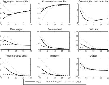
Finally, I assess the role played by the share of non ricardian consumers,λ. A clear result emerges fromfigure 9.
Result 7. Aggregate consumption and λ. Aggregate consumption shows a positive response to a government spending shock for large values of the share,λ, of non ricardian consumers.
Figure 9 makes clear that aggregate consumption shows a positive, and mildly persistent, response for values of the share on non ricardian consumers
which are above the upper interval of empirical estimates. As in GVL the effect of the spending shock on output is increasing in the share of non ricardian con-sumers. This implies also that the effect on labor demand and on the real wage are positive function ofλ. The pattern of the real wage is transmitted to price inflation. Since monetary policy obeys to the Taylor Principle, the real rate grows. For this reason consumption of ricardian consumers is lower the higher the share of non ricardian consumers. This effect counterbalances the increase incrt, which, instead, is a positive function ofλ.
6
Robustness
6.1
The response of aggregate consumption to a spending
shock.
In this section I intend to verify whether the impact response of aggregate consumption is affected by the monetary rule followed by the central bank.
Figure 10 reports the response of aggregate consumption to a government spending shock under the various specifications of the general rule(20)we have analyzed. The response of the central bank to price inflation is kept at its baseline value, while we report impulse response functions for three different specification ofτy. I state the following result.
Result 8. Aggregate consumption and monetary rules. Backward look-ing monetary rules are more likely than contemporaneous and forward looking rules to deliver a positive impact response of aggregate consump-tion to a government spending shock. Reacting to deviaconsump-tions of output from its steady state level reduces, instead, the likelihood of a positive impact response of consumption.
The reason for which a backward looking rule helps obtaining a positive impact response is straightforward. If the central bank responds to lagged vari-ables, monetary conditions are unchanged during the period in which the shock hits the economy, i.e. there is no positive impact increase in the real rate as under the contemporaneous and the backward looking rule. This favours a mild reduction in consumption of ricardian consumers, while that of non ricardian is positively affected by the increase in hours worked and the real wage. However, as the effects of the shock are transmitted to inflation and output, the varia-tion in the real rate of interest determines a reducvaria-tion in level of employment, which drives crt below the steady state level and at the same time causes a
further reduction in co. These effects are mirrored in the dynamic pattern of
aggregate consumption, which exhibits a positive response on impact, but lacks of persistence. Notice that this stands in sharp contrast with what happens if the central bank follows, for example, a contemporaneous rule, where aggregate consumption decreases smoothly after the government spending shock (panel
relevantly for what concerns the likelihood of delivering a positive impact re-sponse of consumption, no matter whether we consider an inertial component in interest rate setting.
Reacting to output deviation determines a less marked increase of production in the aftermath of the shock, containing the variation in hours worked and, thus, in consumption of non ricardian consumers.15
7
Conclusions
I regard a framework where current income affects consumption possibilities as a promising step towards realism in economic modeling. In this case, however, it should be taken into account that labor markets and the wage setting process are subject to some form of imperfections.
In an economy populated by an exogenous share of non ricardian consumers, wage stickiness affects both the response of aggregate variables to a government spending shock and the conditions for equilibrium determinacy.
Once wage stickiness is considered, the positive effect of government spend-ing on aggregate consumption reported by the empirical studies of,inter alia,
Blanchard and Perotti (2002), is not a robust feature of the model with rule of thumb consumers. In particular, it can be replicated just when the marginal disutility of labor effort is low. Contrary to Bilbiie (2005), I have shown that, for a wide set of parameter configurations, an active monetary policy implies a determinate equilibrium. Determinacy regions are similar to those delivered by a standard model, i.e. one where all consumers are ricardian. The latter result is robust to various specification of the Taylor rules which can be found in the literature. Further, it suggests that the feature of the optimal monetary policy in a setting with non ricardian consumers could strongly depend on the assumption relative to the wage setting process.
We conjecture that the optimality of a passive monetary rule, as advocated by Bilbiie (2005) in a sticky prices-flexible wages economy, could be obscured by considering a modest degree of wage stickiness. This is, although in a simpler model, part of my ongoing research.
8
References
Amato, J. D. and Laubach T.(2003). Rule-of-Thumb Behavior and Monetary Policy.European Economic Review, vol. 47, 5, pages 791-83.
Ascari, G. (2000). Optimizing Agents, Staggered Wages and the Persistence innthe real effect of Money Shocks. The economic Journal, 110, pp. 664-686.
Ascari, G. and Ropele T. (2005). Trend Inflation, Taylor Principle and Indeterminacy. Mimeo, University of Pavia.
1 5The case of a central bank reacting to wage inflation can be found on the appendix to the
Baxter,M.,King R., (1993). Fiscal Policy in General Equilibrium. The Amer-ican Economic Review, Vol. 83 (3), pp.315-334.
Bilbiie, F. O. (2005). Limited Asset Market Participation, Monetary Pol-icy,and Inverted Keynesian Logic. Mimeo, Nuffield College, Oxford U.
Bilbiie, F. O. and R. Straub (2005). Fiscal Policy Business Cycle and Labor Market Fluctuations. WP 2004-6, Hungarian National Bank.
Bilbiie, F. O. (2006). Non-Separable preferences, Fiscal Policy puzzles and Inferior Goods. Mimeo, Nuffield College.
Blanchard, O.J. and R. Perotti, 2002. An empirical characterization of the dynamic effects of changes in government spending and taxes on output. Quar-terly Journal of Economics, 117, 1329-68.
Burnside C., Eichembaum, M., and Fisher J. (2004). Fiscal shocks and their consequences. Journal of Economic Theory, pp. 89-117.
Calvo, Guillermo (1983). Staggered Prices in a Utility Maximizing Frame-work. Journal of Monetary Economics, 12, 383-398.
Campbell, J. Y., Mankiw N. G. (1989). Consumption, Income, and Inter-est Rates: Reinterpreting the Time Series Evidence. In O.J. Blanchard and S.Fischer (eds.),NBER Macroeconomics Annual 1989, 185-216, MIT Press.
Carlstrom C.T., and Fuerst T., (2005). Investment and Interest rate policy: a discrete time analysis. Journal of Economic Theory 123, pp. 4-20.
Christiano, L.J., M. Eichenbaum, and C. Evans, (2005). Nominal Rigidities and the Dynamic Effects of a Shock to Monetary Policy. Journal of Political Economy vol. 113, no.1.
Coenen, G. and Straub R. (2004). Non-Ricardian Households and Fiscal Policy in an Estimated DSGE Model of the Euro Area. Mimeo.
Colciago, A.,Muscatelli, V.A., T. Ropele and P. Tirelli (2006). The Role of Fiscal Policy in a Monetary Union: Are National Automatic Stabilizers Eff ec-tive?. CESifo wp 1682.
Erceg,C.J., Dale W.H., and Levin A. (2000). Optimal monetary policy with staggered Wage and Price Contracts. Journal of Monetary Economics 46, pp. 281-313.
Fatás, A. and I. Mihov, 2001. Government size and automatic stabilizers: international and intranational evidence. Journal of International Economics, 55, 3-28.
Galí, J., D. López-Salido, and J. Valles, (2004). Rule-of-Thumb Consumers and the Design of Interest Rate Rules. Journal of Money, Credit and Banking, Vol. 36 (4), August 2004, 739-764.
Galí, J., D. López-Salido, and J. Valles, (2005). Understanding the Effects of Government Spending on Consumption. Forthcoming on theJournal of the European Economic Association.
Linneman, L. (2006). The Effects of government spending on private Con-sumption: a puzzle?. Forthcoming inJournal of Money Credit and Banking.
Linneman, L. and Schabert, A. (2006). Fiscal policy and the new neoclassical Synthesis. Journal of Money Credit and Banking, Vol 35 (6), 911-929.
Mankiw,G. (2000). The Savers-Spenders Theory of Fiscal Policy. The Amer-ican Economic Review, Vol. 90 (2), pp.120-125.
Muscatelli, A., P. Tirelli and C. Trecroci, (2003). Can fiscal policy help macroeconomic stabilization? Evidence from a New Keynesian model with liq-uidity constraints. CESifo wp No. 1171.
Schmitt-Grohe, S. and M. Uribe (2004a). Optimal operational monetary policy in the Christiano-Eichenbaum-Evans model of the U.S. business cycle.
NBER wp No. 10724.
Schmitt-Grohe, S. and M. Uribe (2004b). Optimal simple and implementable monetary andfiscal rules. NBER wp No. 10253.
Taylor, J. B. (1999). A historical analysis of monetary policy rules. In J. B. Taylor (Ed.),Monetary Policy Rules, pp. 319-341. Chicago: University of Chicago Press.
Wolff, E. (1998). Recent Trends in the Size Distribution of Household Wealth. Journal of Economic Perspectives 12, pp. 131-150.
Woodford, M. and J. Rotemberg (1997). An Optimization-Based Econo-metric Model for the Evaluation of Monetary Policy. NBER Macroeconomics Annual 12: pp.297-346.
Woodford, M., (2003). Interest and Prices. Princeton University Press.
Appendix.
Log-linearized equilibrium conditions.
This appendix provides a log-linear approximation to the equlibrium conditions of the model economy described in the text. For a detailed derivation see also GVL.
Under the assumed functional forms, the Euler equation for Ricardian house-holds takes the log-linear form
cot−Etcot+1=−Et(rt−πt+1) (21)
Log-linearization of equations(6)and(8)leads to the dynamic of (real)Tobin’s Q
qt= (1−β(1−δ))Etrtk+1+βEtqt+1−(rt−Etπt+1) (22)
and its relationship with investment:
ηqt=it−kt−1
Equation(10)determines the following log-linear form for consumption of non ricardian agents crtt = (1−α) µpγc (lt+ωt)− 1 γct r t (23)
while the assumption that consumption level are equal at the steady state im-plies that aggregate consumption is
The stock of capital evolves according to
δit=kt−(1−δ)kt−1 (25)
Log-linearization of the aggregate resource constraint around the steady state yields
yt=γcct+gt+ (1−γec)it (26)
whereeγc=γc+γg. As in shown by Woodford (2003) a log-linear approximation to the aggregate production function is given by
yt= (1−α)lt+αkt−1 (27)
Assuming that steady state stock of debt is zero and a steady state balanced government budget, the dynamic of debt around the steady state yields the following law of motion for the stock of debt
bt= (1 +ρ) (bt−1+gt−tt) (28)
The New Keynesian Phillips is obtained through log-linearization of condition
(2)and reads as πt=κpmct+βEtπt+1 (29) whereκp= ( 1−βξp)(1−ξp) ξp andmct= (1−α)wt+αr k
t is the real marginal cost.
Equations (21) through(29), equation (19) together with the policy rules
Figures
0 1 2 3 4 5 0 0.1 0.2 0.3 0.4 0.5 0.6 0.7 0.8Elasticity of marginal disutility of labor (φ)
Sensitivity of real wage to output (
ψ ) ξ w=0 ξw=0.5 ξw=0.75
Figure 1: Sensitivity of real wage with respect to output as a function of the elasticity of marginal disutility of labor.
0 0.5 1 1.5 2 2.5 3 0 0.1 0.2 0.3 0.4 0.5 0.6 0.7 0.8 0.9 ξw=0.75
Inflation coefficient response (τπ)
Share of non ricardian consumers (
λ
)
Determinacy region
Figure 2: Determinacy region when wages have an average duration of 4 quarters (ξw= 0.75). Instability area in black.
0 1 2 3 4 5 6 0 0.2 0.4 0.6 0.8 a): ξw=0 ξp=0.75 0 1 2 3 4 5 6 0 0.2 0.4 0.6 0.8 b): ξw=0.5 ξp=0.75
Inflation coefficient response (τπ)
Share of non ricardian consumers (
λ ) 0 1 2 3 4 5 6 0 0.2 0.4 0.6 0.8 b): ξw=0.9 ξp=0.75 Indeterminacy Region Determinacy regions Determinacy Regions
Figure 3: Indeterminacy regions under alternative degree of wage stickiness. In-stability areas in black. Panela (ξw= 0), panelb(ξw= 0.5)panelc(ξw= 0.9).
0 0.2 0.4 0.6 0.8 0 0.2 0.4 0.6 0.8 a): ξw=0 0 0.2 0.4 0.6 0.8 0 0.2 0.4 0.6 0.8 b): ξw=0.5
Share of non ricardian consumers (
λ ) 0 0.2 0.4 0.6 0.8 0 0.2 0.4 0.6 0.8 c): ξw=0.75 Price stickiness (ξp) 0 0.2 0.4 0.6 0.8 0 0.2 0.4 0.6 0.8 d): ξw=0.9 Determinacy region Determinacy region
Determinacy region Determinacy region
Figure 4: Indeterminacy regions under alternative degree of wage stickiness. Panela (ξw= 0); panelb (ξw= 0.5); panelc (ξw= 0.75); paneld (ξw= 0.9).
0 0.2 0.4 0.6 0.8 0 0.2 0.4 0.6 0.8 a): ξw=0 ξp 0 0.2 0.4 0.6 0.8 0 0.2 0.4 0.6 0.8 b): ξw=0.5 ξp 0 0.2 0.4 0.6 0.8 0 0.2 0.4 0.6 0.8 c): ξw=0.75 ξp 0 0.2 0.4 0.6 0.8 0 0.2 0.4 0.6 0.8 d): ξw=0.9 ξp
Share of non ricardian consumers
φ=0.2 φ=1 φ=4.84
Determinacy region
Determinacy region
Determinacy region Determinacy region
5 10 15 20 −0.8 −0.6 −0.4 −0.2 0 Aggregate Consumption 5 10 15 20 −2 −1.5 −1 −0.5 0 Consumption Ricardian 5 10 15 20 −1 −0.5 0 0.5 1
Consumption non Ricardian
5 10 15 20 −0.2 0 0.2 0.4 0.6 Real wage 5 10 15 20 0 0.5 1 Hours 5 10 15 20 0 0.1 0.2 0.3 0.4 Real rate 5 10 15 20 0 0.2 0.4 0.6 0.8
Real marginal cost
5 10 15 20 0 0.2 0.4 0.6 0.8 Inflation
% deviation from steady state
5 10 15 20 −0.2 0 0.2 0.4 0.6 Output
Figure 6: Impulse response functions to a government spending shock. Baseline parametrization. 0 5 10 15 20 −1 −0.5 0 0.5 1 Aggregate consumption 0 5 10 15 20 −2 −1 0 1 Consumption Ricardian 0 5 10 15 20 −1 0 1 2
Consumption non Ricardian
0 5 10 15 20 −0.2 0 0.2 0.4 0.6 Real Wage 0 5 10 15 20 0 1 2 3 Hours 0 5 10 15 20 −0.1 0 0.1 0.2 0.3 Real rate 0 5 10 15 20 −0.5 0 0.5 1 Real MC 0 5 10 15 20 −0.2 0 0.2 0.4 0.6 Inflation 0 5 10 15 20 −0.5 0 0.5 1 1.5 output
% deviation from steady state
φ=4.84 φ=1 φ=0.2
Figure 7: Impulse response functions to a government spending shock. Sensi-tivity toφ.
0 5 10 15 20 −1.5 −1 −0.5 0 0.5 Aggregate consumption 0 5 10 15 20 −4 −3 −2 −1 0 Consumption ricardian 0 5 10 15 20 −1 0 1 2
Consumption non ricardian
0 5 10 15 20 −0.5 0 0.5 1 1.5 Real wage 0 5 10 15 20 0 0.5 1 1.5 Employment 0 5 10 15 20 0 0.2 0.4 0.6 0.8 real rate 0 5 10 15 20 0 0.5 1 1.5
Real marginal cost
0 5 10 15 20 0 0.5 1 Inflation 0 5 10 15 20 −0.5 0 0.5 1 Output
% deviation from steady state
λ=0.5 λ=0 λ=0.8
Figure 8: Impulse response functions to a government spending shock. Sensi-tivity toλ. 0 0.5 1 1.5 2 2.5 3 0 1 2 3 (a)i=−1: ρr=0.5 0 0.5 1 1.5 2 2.5 3 0 1 2 3 (b) i=−1: ρr=0 0 0.5 1 1.5 2 2.5 3 0 1 2 3 (c) i=0 ρr=0.5 0 0.5 1 1.5 2 2.5 3 0 1 2 3 (d) i=0 ρr=0
Output−gap response coefficient (
τy ) 0 0.5 1 1.5 2 2.5 3 0 1 2 3 (e) i=+1 ρr=0.5
Inflation response coefficient (τπ)
0 0.5 1 1.5 2 2.5 3 0 1 2 3 (f) i=+1 ρr=0 Determinacy region Determinacy region Instability region
Determinacy region Determinacy region
Determinacy region
Determinacy region
Figure 9: Indeterminacy regions under alternative monetary rules. i = −1: backward looking rule; i = 0 contemporaneous rule; i = +1 forward looking rule
0 2 4 6 8 10 12 −1 −0.8 −0.6 −0.4 −0.2 0 (a) i=−1 ρr=0.5, τπ=1.5 0 2 4 6 8 10 12 −1 −0.5 0 0.5 (b) i=−1 ρr=0, τπ=1.5 0 2 4 6 8 10 12 −1 −0.8 −0.6 −0.4 −0.2 (c) i=0 ρr=0.5, τπ=1.5 0 2 4 6 8 10 12 −0.8 −0.6 −0.4 −0.2 0 (d) i=0 ρr=0, τπ=1.5
% deviation of aggregate consumption form steady state
0 2 4 6 8 10 12 −1 −0.5 0 (e) i=+1 ρr=0.5, τπ=1.5 0 2 4 6 8 10 12 −0.7 −0.6 −0.5 −0.4 −0.3 (f) i=+1 ρr=0, τπ=1.5 τy=0.1 τy=0.3 τy=0.5
Figure 10: Response of aggregate consumption under alternative monetary rules. i = −1: backward looking rule; i = 0 contemporaneous rule; i = +1