Assessment of element-specific recycling efficiency in WEEE pre-processing

(1)

Maximilian Ueberschaar, Julia Geiping, Malte Zamzow, Sabine Flamme, Vera

Susanne Rotter

Assessment of element-specific recycling

efficiency in WEEE pre-processing

Article, Postprint

This version is available at https://doi.org/10.14279/depositonce-6365.

Suggested Citation

Ueberschaar, Maximilian; Geiping, Julia; Zamzow, Malte; Flamme, Sabine; Rotter, Vera Susanne: Assessment of element-specific recycling efficiency in WEEE pre-processing. - In: Resources, Conservation, and Recycling. - ISSN: 0921-3449. - 124 (2017). - pp. 25-41. - DOI:

10.1016/j.resconrec.2017.04.006. (Postprint version is cited, page numbers may differ.)

Terms of Use

German copyright applies. A non-exclusive, non-transferable and limited right to use is granted. This document is intended solely for personal, non-commercial use.

(2)

Page 2 of 30

Abstract

Pre-processing is a crucial step to ensure the efficiency of subsequent processes and the quality of recyclates. The efficiency of pre-processing can be affected by high losses to undesignated output fractions. Standard batch tests usually provide mass balances and are a good proxy for bulk materials balances (iron/steel, aluminum, plastics).

This article aims at harmonizing methodologies and recommends a strategy for further study in pre-processing on a plant scale. We have developed an “extended batch test” method, which should help to

• describe the fates of materials and elements,

• assess the quality of output fractions,

• identify access points for critical metals and other valuable elements to enable their recovery. A methodical approach was compiled with common material flow analysis methods and an extended set of methods, which improve the reliability via the assessment of uncertainties. This applies to systematic effects and random effects. This extended batch test was performed with a 40 Mg Waste Electrical & Electronic Equipment (WEEE) batch to trace the flows of industrial base metals, precious metals and critical metals in a WEEE pre-processing plant.

Results show that one-third of the input was separated and sorted manually, while the remaining material was subsequently crushed and automatically sorted. Copper and precious metals are distributed to various output fractions but are most concentrated in the sorting residues. Critical metals like cobalt and rare earth elements are mainly concentrated in the manually sorted materials but also appear in the ferrous metals scrap and the shredder light fraction.

Graphical abstract Validation of base data Quantification of uncertainties Calculation of mass balance Uncertainty propagation Match of mass balance Sorting Disassembly Sieving Sample preparation Chemical analyses

Experimental flow characterization

Literature Internal data originating from other experiments Secondary data Governmental / statistical institutions

Mass / substance flow

4. Visualization Cu 31% Si 22% Al 15% Ca 10% Zn 9% Fe 3% Mg 3% Pb 2% Ti 2% CuSiAl CaZnFe MgPbTi SnBaSb NiMnAg MoAuLa PdCeNd 0 1 10 100 1,000 10,000 100,000 CuSiAlCaZnFeMgPbTiSnBaSbNiMnAgMoAuLaPdCeNd M ass fractio n [p pm ] Sorting residues (mixed plastics) Chemical composition 0 5,000 10,000 15,000 20,000 25,000 30,000 35,000 40,000 45,000 0 10 20 30 40 50 M ass fractio n o f elem ent [ppm ]

Distribution of total element potential [%]

Cobalt Laptops Tablet Desktop PC Mobile Phone Smart Phone TV TFT Batteries Ferrous metals SLF (Fluff) 0 200 400 600 800 1,000 1,200 1,400 1,600 0 10 20 30 4050 M as s fra ct ion of ele ment [ppm ]

Tantalum Pre-sorted PCB Laptops Tablet Desktop PC Scanner Mobile Phone Smart Phone

Hot spot plots

0% 10% 20% 30% 40% 50% 60% 70% 80% 90% 100% 0.0 1.0 100.0 Cu mmu la tiv e mass (% ) Grain diameter (mm) Ce Eu La Nd 0% 10% 20% 30% 40% 50% 60% 70% 80% 90% 100% 0.0 0.1 1.0 10.0100.0 Cu mmu lativ e mass (% ) Grain diameter (mm) Ga Co REE Total mass PCB Heterogeneity

1. Physical and chemical characterization

2. Uncertainty assessment

3. Mathematical model

Extended batch test Input material Output material Sampling Weighing Batch test

(3)

Page 3 of 30

1. Introduction

Pre-processing is one of the central steps in the recycling chain of Waste Electrical and Electronic Equipment (WEEE) as well as of other complex products. Through liberation and separation, secondary raw materials are channeled into designated recovery processes. Generated outputs have to be either processed further or can be used directly in final recovery operations. To fulfill the regionally mandatory recycling quotas, current recycling strategies target industrial base metals like copper, iron, and aluminum, and also plastics, as bulk materials (Chancerel, 2010; Reuter and van Schaik, 2012; Rotter et al., 2016). Furthermore, trace materials with a high economic value, such as precious metals (gold, silver, palladium), are of high interest from an economic and ecologic perspective (Li et al., 2015). A recovery of such materials takes place in subsequent end-refining processes, which are usually limited to a particular set of materials (Khaliq et al., 2014). For example, integrated smelters are capable of recovering copper, precious metals, and some additional elements. However, other materials and elements carried in the same material stream are diluted to the slag and irretrievably lost. Because of this, the transfer of non-target metals into recyclates for end-processing leads to a loss of these materials, higher energy demands and lower recovery rates due to impurities and potential end-products of lower quality (UNEP, 2013). This applies in particular to most of the metals defined as critical raw materials (CRM) by the European Commission (2010, 2014), the U.S. Department of Energy (2011) and the Japan Institute of Metals and Materials (Hatayama and Tahara, 2015) and whose recovery is discussed on the political agenda. The set and classification of assessed materials differ in these criticality studies. Therefore, we will distinguish them as follows: “industrial base metals (IBM)” (aluminum, iron, copper), “precious metals (PM)” (for example gold, silver, and palladium) and a selected “set of critical metals (S-CRM)” (for example, rare earth elements (REE), indium, cobalt, etc.). S-CRMs are mainly applied in complex WEEE products (Chancerel et al., 2015, 2013). Due to highly sophisticated processes for their recovery, no recycling strategies are implemented yet (Kumar and Holuszko, 2016; Li et al., 2017; Zeng and Li, 2016).

The overall WEEE recycling efficiency can be measured at three levels: 1. collection rate, which represents the ratio between generated WEEE and WEEE collected for recycling. 2. recycling process efficiency rate, which is the quotient of a recycled material and that material collected with WEEE for recycling. 3. (element-specific) recycling rate, which generally refers to functional recycling and is defined by the ratio of recycled material (or element) and the total amount of this material (or element) in generated WEEE. (UNEP - International Resource Panel, 2011)

Although Reuter and van Schaik highlighted that recovery rates could only be assessed by considering the overall process chain, an assessment of the performance at the pre-processing level is a useful tool to identify design-related reasons for resource losses due to insufficient liberation (Reuter and van Schaik, 2015; van Schaik and Reuter, 2010) or to optimize plant operations (Chancerel et al., 2009; Chancerel and Rotter, 2009).

In process engineering, mass and energy balances represent essential tools for checking the efficiency of processes. Recycling efficiency is usually tested with batch tests. Due to local legislation, recycling schemes or internal quality management, plant operators are increasingly required to perform such batch tests (NVMP Association, 2014), with WEEELABEX standards being one example for technical implementation. These are defined as the “manual or mechanical processing of a definite and well-defined amount of WEEE or fractions thereof to determine the yields and compositions of the resulting output fractions and de-pollution performance” (WEEEforum, 2013). Such batch tests represent a mass balance of processed material. The informative value of this approach is limited, as no full information about material or substance flows can be provided. A higher level is achieved through partially conducted sorting analyses of particular generated output fractions. Furthermore, the quality

(4)

Page 4 of 30

of relevant waste fractions regarding de-pollution can be verified by carrying out chemical analyses (WEEEforum, 2013).

Experimental material flow analysis has been introduced as a systematic approach to track goods/materials and substances to understand their origin and fate in investigated processes. It is based on the same procedures used for conventional batch tests, which means a mass balance of goods. Also, the MFA can focus on individual substances (chemical elements, alloys, compounds, etc.) which is often called substance flow analysis (SFA) (Brunner and Rechberger, 2004). Information about individual substances in processed goods is mainly based on individually executed investigations and chemical measurements. (Brunner, 2012)

In order to compare commonly used methodologies and the quality of the results of MFA on a substance level, various studies using experimental batch tests have been compared in Table 1. The trials took place in different facilities processing household waste, WEEE and ELV (end-of-life-vehicles). Table 1: Comparison of experimental MFA on a substance level in the form of a batch test applied on various waste streams

Study Waste input Objective Size of _batch Target _elements Sampling _method _preparationSample Digestion Analytical _methods Input _sampling Output _sampling Statistical _analysis

(Rotter et al., 2004) Household waste Assessment of selective Heavy metal Separation in RDF 4-8 Mg Cl, Hg, Cd, Pb, Zn, (Sb) 3 samples per fraction Grinding <0,5 mm Acid based Microwave digestion AAS Sorting analysis of waste fraction Yes, all fractions Calculation of interval of confidence (95%) (Morf and Taverna, 2004) sWEEE Assessment of metallic and non-metallic materials 230 Mg Al, Sb, Pb, Cd, Cr, Fe, Cu, Ni, Hg, Zn 16-20 single samples per fraction Manual sorting, grinding, partially re-melting Acid based Microwave digestion ICP-MS, ICP-OES, XRF Sorting analysis Yes, only relevant fractions Calculation of interval of confidence (95%) (Chancerel, 2010; Chancerel et al., 2011, 2009) sWEEE, ICT & consumer electronics Identification of PM losses in pre-processing 27 Mg Ag, Au, Pd, Cu, Fe, Al

Umicore standard including fire assaying and re-melting with recuperation of target elements. X-ray fluorescence analysis and acid based digestion prior to determination with inductively coupled plasma mass spectrometry (ICP-MS) and atomic emission spectroscopy (ICP-AES)

No (data on average input compositio n assessed Full sampling, dismantling tests, literature data, visual estimation Data reconciliation of material balance based on Gaussian distribution (Schoeps et al., 2010) Mono batch: PC Identification of PM losses in pre-processing 2.9 Mg Ag, Au, Pd Sorted

mono batch No info. Not applied

(Oguchi et al., 2013) WEEE: PCB & CRT Metal fates in actual waste treatment processes No info. Full analysis No info. Grinding <0,25 mm Acid based Microwave digestion ICP-OES, ICP-MS Sorting analysis Yes, all

fractions Not applied

(Morf et al., 2013) Municipal solid waste Precious metals and rare earth metals flow No batch trial Full analysis Method following (Bauer, 1995; Gy, 1992) Partially divided; grinding <0,1 mm Acid based Microwave digestion

ICP-MS Only homogeneous materials; full chemical analysis Data reconciliation based on Gaussian distribution (Arena and Di Gregorio, 2014) Municipal solid waste Mass flow rates and composition for decision making 100

Mg C, Cd, Pb Literature review No No info. Data reconciliation based on Gaussian distribution (Widmer et al., 2015) EE in ELV Distribution of scarce metals. Plausibility of results 95,3 Mg; 100 ELV 31 scarce metals No info. Grinding <0,5 mm Acid based Microwave digestion XRF, OES, ICP-MS Generic input 6 from 7 sampled

ISO GUM class

c, 12−24% (Habib et al., 2015) Hard disk drives Track of REE based permanent magnets 244 kg; 1050 HDD

REE No info. No info. - WD-XRF Yes Visual _sorting Not applied Note: household waste = residual household waste is mixed waste collected after source separations, WEEE = small WEEE, ICT = information and

communications technology, consumer electronics = entertainment electronics

Some conclusions from previous MFA studies can be summarized as follows:

- Assessment of uncertainties and an appropriate uncertainty propagation received only minor attention.

- In order to generate data with a high level of detail, a combination of various methodologies has to be used. Through this, uncertainties like systematic effects can be reduced.

- Furthermore, it is important to validate results. One possibility is the sampling of the input material in order to match the results of input and output.

(5)

Page 5 of 30

Therefore, the objective of this article is to demonstrate a suitable methodology for WEEE pre-processing that supports improvements in recycling efficiencies for bulk and trace materials along the recycling chain with particular attention to CRM, which presently has low recycling rates. For this, we took the standard WEEELABEX batch test (WEEEforum, 2013) as a basis and developed an “extended batch test”, which should help to

• describe the fate of materials and elements during pre-processing,

• assess the quality of output fractions from pre-processing relative to the subsequent process steps and

• identify options for further concentration of CRMs and other valuable elements to enable their recovery

Furthermore, this article should help to harmonize existing methodologies and recommend a useful strategy for further study in pre-processing on a plant scale.

2. Material and Methods

2.1. Research concept

For this study, a batch test was conducted in a WEEE pre-processing plant. The processes used covered liberation and manual and automated sorting, which can be regarded as typical in the pre-processing sector. The input material was 40 Mg WEEE comprising a mix of information and telecommunication technology devices, consumer entertainment devices, small household appliances, electrical and electronic tools, toys and electric motors, etc. Only a few non-designated devices were present in the batch, such as air conditioning and cooling appliances and lamps, which were separated in the manual sorting step.

Figure 1 shows the process scheme of the study plant with the input and output streams generated by the various separation processes. The output materials are grouped as output fractions from “manual sorting” (MS) and “automated sorting” (AS). A coding for all output fractions in the extended batch test is depicted in the supporting information S2.

Figure 1: Process set-up of recycling plant investigated

Target metals of this investigation include ‘industrial base metals’ (IBM) like aluminum, iron and copper, ‘precious metals’ (PM) gold, silver, palladium and platinum and a selected ‘set of critical metals’ (S-CRM) like cobalt, gallium, indium, tantalum and the WEEE relevant REE (neodymium, praseodymium, dysprosium, lanthanum, cerium, europium, lutetium, etc.).

Input Ou tp u t Ou tp u t Output Magnet separator Air classifier Manual sorting Eddy current separator Pre-crushing Manual sorting Inductive optoelectronic separator Nd-Magnet separator Granulator

Devices, components, compounds

Filter dust Plant dust extraction system

Sorting residues (mixed plastics) Ou tp u t Shredder light fraction (SLF) Ou tp u t Ferrous metals scrap Ou tp u t Low magnetic material Ou tp u t Non-ferrous metals scrap Ou tp u t Shredded Printed Circuit Boards General losses / sweepings E-motors Tools scrap Loud-speaker …

(6)

Page 6 of 30

Various experimental MFA have been conducted in recent years with different objectives and waste streams. Based on the information in Table 1, a general methodology for carrying out a batch test was developed. Figure 2 depicts the complete approach.

Figure 2: Experimental design of the “extended batch test” with subsequent data collection and evaluation

Based on a chemical characterization, the composition of all input and output materials can be assessed. For output fractions consisting of whole devices or components, disassembly prior to chemical analyses might be necessary. Additional sorting and sieving analyses represent adequate tools to increase information density and enable a validation of data.

Chemical analyses of all output fractions are not always possible. In such cases, sufficient data must be available from own studies or external research. This secondary data has to be calculated with the experimental data within an appropriate mathematical model. Through this, the overall flows and stocks can be assessed.

Uncertainties are usually not part of MFA studies (Laner et al., 2014). However, in order to provide comprehensible quantitative data, the apportioning of uncertainties is necessary. Therefore, the mathematical model used must contain an adequate assessment and propagation of uncertainties.

2.2. Sampling methodologies

In this study, sampling followed the method of LAGA PN 98, which represents the only national regulation for the sampling of waste materials in Germany. It provides a general guideline for procedures for the investigation of physical, chemical and biological properties of waste (Länderarbeitsgemeinschaft Abfall, 2001). According to the grain size distribution, heterogeneity of material and the substances to be investigated, appropriate sampling procedures needed to be chosen according to the kind of transport or storage (head, belt, falling stream, etc.) and material characteristics. On this basis, minimum sample quantities for each output fraction were calculated following LAGA PN 98. Validation of base data Quantification of uncertainties Calculation of mass balance Uncertainty propagation Match of mass balance Mathematical model Input material Output material Sampling Weighing Batch test Sorting Disassembly Sieving Sample preparation Chemical analyses

Experimental flow characterization

Literature Internal data

originating from other experiments Secondary data Governmental / statistical institutions

Mass / substance flow

Visualization Cu 31% Si 22% Al 15% Ca 10% Zn 9% Fe 3% Mg 3% Pb 2% Ti 2% CuSi Al CaZn Fe MgPb Ti Sn Ba Sb Ni Mn Ag MoAu La PdCe Nd 0 1 10 100 1,000 10,000 100,000 CuSiAlCaZnFeMgPbTiSnBaSbNiMnAgMoAuLaPdCeNd M ass fractio n [p p m ] Sorting residues (mixed plastics) Chemical composition 0 5,000 10,000 15,000 20,000 25,000 30,000 35,000 40,000 45,000 0 10 20 30 40 50 M ass fractio n o f elem ent [p pm ]

Cobalt Laptops Tablet Desktop PC Mobile Phone Smart Phone TV TFT Batteries Ferrous metals SLF (Fluff) 0 200 400 600 800 1,000 1,200 1,400 1,600 0 10 20 30 40 50 M as s fra ct io n of ele m ent [ppm ]

Tantalum Pre-sorted PCB Laptops Tablet Desktop PC Scanner Mobile Phone Smart Phone

Hot spot plots

0% 10% 20% 30% 40% 50% 60% 70% 80% 90% 100% 0.0 1.0 100.0 C u mmu la tiv e mass (% ) Grain diameter (mm) Ce Eu La Nd 0% 10% 20% 30% 40% 50% 60% 70% 80% 90% 100% 0.0 0.1 1.0 10.0 100.0 C u mmu la tiv e mass (% ) Grain diameter (mm) Ga Co REE Total mass PCB Heterogeneity Composition data Mass data

(7)

Page 7 of 30

2.2.1. Calculation of required primary sample amounts

Relevant parameters were established prior to the batch test, to obtain information about the homogeneity of the materials to be sampled, predicted volume and mass per output, bulk density and grain size distribution. From this, a minimum number of single samples of equal volume and the total size of the sample taken per output were calculated. The amount of single samples taken was divided by the duration of the batch test (cf. supporting information S3).

The pre-assessment revealed a high inhomogeneity for particular output materials. According to Chancerel, 2010, sorting residues and ferrous metals scrap are carriers of high loads of target metals (cf. Figure 1). Increasing the reliability of the sampling procedure, the calculation of the amount of increments was carried out conservatively. Furthermore, the volume of the increments was increased. The sampling of single devices and components of input material and material deriving from manual separation is unusual in sampling procedure. As these flows represent no continuous stream, LAGA 98PN suggests a single sampling of these fractions. Therefore, material from the manual separation was sampled in high quantities, to carry out product-centric recyclability assessments with disassemblies and partial chemical analyses (Rotter et al., 2013). Table 2 shows a sampling procedure overview and the sampled masses.

Table 2: Overview of sampled fractions over an 11 h sampling period

Sampled Output Output batch test Bulk density Volume of total output Single sample volume Number single increments Average interval of sampling Overall sampling quantity before reduction Sample

code Sample name [kg] [kg/m³] [m³] [L] [-] [min] [L] [kg]

Manua l s ort ing MS1 Tools scrap 789 not applied 33 MS2 E-Motors 1,645 549 MS3 Loudspeaker 397 237 MS4 Copper rich fraction 3,271 47 MS5 Pre-sorted Printed Circuit Boards 221 283 Automated s ort ing

AS1 Ferrous metals

scrap 9,789 1,500 6.5 7 22 30 154 228

AS2 Low magnetic

material 709 1,000 0.7 3.5 22 30 77 77 AS3 Non-ferrous metals scrap 1,105 1,500 0.7 4 22 30 88 108 AS4 Shredded Printed Circuit Boards 625 500 1.3 8 22 30 176 87 AS5 Sorting residues (mixed plastics) 12,498 440 28.4 22 22 30 484 208 AS6 SLF (Fluff) 1,691 210 8.1 6 22 30 132 67

AS7 Filter dust 96 210 0.5 5 6 100 30 8

AS8 Sweepings ~100 not applied 33

Note: SLF = shredder light fraction

2.2.2. Subsampling from primary samples

In order to provide sufficient representative material for the characterization of the output fractions, the samples taken were split for chemical analyses, sieving analyses and sorting analyses, with some

(8)

Page 8 of 30

partial samples retained. The division of the samples was carried out using a ripple divider for handling large sample volumes (cf. supporting information S4). Table 3 shows the sample masses for the characterization tests subsequently carried out.

The chemical analyses were conducted in up to three laboratories, depending on the elements to be measured and the complexity of the sample.

Table 3: Sample splitting for chemical and sorting analyses

Sample code Mass for sieving and sorting analysis [kg] Chemical analyses Total mass for

chemical analysis [kg] Laboratory 1 [kg] Laboratory 2 [kg] Laboratory 3 [kg] AS1 66 84 74 10 10 AS2 37 41 41 - - AS3 54 54 54 - - AS4 22 50 43 7 - AS5 51 71 58 13 - AS6 14 33 30 3 - AS7 - 8 6 2 AS8 - 33 33 - - MS5 - 67 67 - -

The unlisted output fractions were not split and were used directly for the chemical analyses.

2.3. Characterization of input and output fractions from the extended batch test

Characterization of output materials provides the database for the MFA. The information was gathered through physical and chemical characterization of the input materials and output fractions from manual sorting (MS) and automated sorting (AS). A full analysis is not always possible or feasible. Therefore, different methodologies were used.

2.3.1. Physical characterization

(1) Batch input characterization

A total of 40 Mg input material was manually sorted prior to the batch test to identify the equipment types present (for example cooling device, CRT TV, tablet, smartphone, etc.) and to determine average weights of the WEEE products in the batch. The material was later remixed to provide a realistic input. The supporting information S1 shows the sorting protocol used.

(2) Disassembly and material quantification (MS)

Dismantling trials were used as a tool to assess the material composition of whole devices and components from manual sorting. Samples were disassembled until manual separation with mechanical tools was no longer possible. Target end materials were components like printed circuit boards (PCBs) and batteries, but mostly homogeneous materials like ferrous metals, non-ferrous metals, plastics and composite materials, which represent an inseparable compound of homogenous materials. The assessment of the output fractions was based on visual identification in combination with a magnet for verifying ferrous metals.

The supporting information S6 shows the disassembly protocol draft. The composition data assessed for small household tools, loudspeaker drivers, and e-motors is depicted in S7.

(3) Sieve analysis (AS)

The output fractions AS1 - 6 were sieved in a Haver “Test Sieve Shaker EML 450 DIGITAL PLUS” using sieves with nominal mesh widths of 0.125; 0.25; 0.5; 1.0; 2.0; 5.0; 8.0; 10; 16; 20 mm. Sieving time was about 5 minutes with self-readjusting amplitude up to maximal 2 mm.

(9)

Page 9 of 30

Due to high shares of fines between 0.25 and 5.0 mm, an additional sieve analysis with nominal mesh sizes 0.2; 0.5; 1.0; 4.0; 6.3; 8.0; 10; 16 mm was carried out for the materials AS4-7 with a KH “Tfk. Rö/W-B” in combination with a subsequent determination of the chemical composition. Sieve time was 10 minutes for 4.0-16 mm and 12 minutes for <4.0 mm with sample sizes AS4 (7.3 kg), AS5 (12.5 kg), AS6 (2.3 kg) and AS7 (1.6 kg), which did not originate from the extended batch test, but from the same processing plant with comparable input material.

(4) Sorting analysis (AS)

Output fractions from the automated sorting processes >5 mm were sorted by visual identification. This excluded the materials AS6 - 8. A sorting protocol was developed, which was used for the analysis (cf. supporting information S5). Main categories for sorting were: ferromagnetic material; aluminum; other non-ferrous metals; colored plastics, black plastics; foils, rubber, etc.; PCBs; batteries; cables; glass, ceramics; organic material; and the rest.

2.3.2. Chemical characterization

(1) Hotspot characterization of disassembled materials (MS)

In addition to the visual material quantification in the dismantling trials, hotspots like metallic pieces or other materials like magnets were determined via an XRF handheld (Thermo Fisher/Analyticon XL3 air) to quantify alloying elements and verify first results.

(2) Literature data on chemical composition (MS)

Not all output fractions from the manual sorting were assessed through disassembly trials with subsequent chemical analyses. Generally, for well-investigated output fractions, in particular whole devices and components, a literature research was carried out. This applied to IT devices like mobile phones, notebooks, etc., and also for single components like batteries or particular output materials, which were assessed in previous batch tests. The supporting information S7 shows the data aggregated for further calculations.

(3) Characterization of sieving steps (AS)

For the characterization of the output fraction of each sieving step in the sieve analysis, samples were dissolved in microwave-assisted aqua regia with 1.600 W, 20 bar, 15:00 min in a CEM MARS 5. For the elemental determination, an ICP-AES (Thermo Scientific iCAP 6000 Series) was used.

(4) Full analysis of output fractions (AS)

Full analyses were carried out on the output fractions from the automated sorting processes (AS1 – 8). To address matrix influences on the measured contents of specific elements, chemical analyses were carried out by three different laboratories using different sample assaying and analytical methods for Ag, Al, As, Au, Ba, Bi, Ca, Cd, Ce, Co, Cu, Eu, Dy, Fe, Ga, Ge, La, Mg, Mn, Mo, Nd, Ni, Pb, Pd, Pr, Pt, Sb, Si, Sm, Sn, Ta, Tb, Te, Ti, V, W, Zn, Zr. Also, loss of ignition (LOI) was determined by laboratory 1 during the assaying step.

Laboratory 1 applied a fire assay and remelting with a recuperation of target elements. An X-ray fluorescence analysis (XRF) and a wet-chemical digestion with a subsequent determination through inductively coupled plasma mass spectrometry (ICP-MS) and atomic emission spectroscopy (ICP-AES) were carried out.

Laboratory 2 analyzed smaller sample sizes to compare the results with laboratory 1. For sample preparation, samples AS4 - 7 were milled in a cross beater mill (Retsch SK1) and an ultracentrifugal mill (Retsch ZM1)with the addition of dry ice in the case of a high plastics content to <0,2 mm powder. Sample AS1 was completely melted at 1700°C without any additives in a standard atmosphere, then homogenized and subsequently cast in a homogeneous solid state. The product was analyzed with an XRF handheld (Thermo Fisher/Analyticon XL3 air). Single pieces were drilled out for a wet-chemical

(10)

Page 10 of 30

analysis at laboratories 2 and 3. Subsequently, all samples were digested with HNO3-H2O and aqua regia in a microwave-assisted digestion with 1.600 W, 20 bar, 15:00 min in a CEM MARS 5. For the elemental determination, an ICP-AES (Thermo Scientific iCAP 6000 Series) was used.

Laboratory 3 received the prepared single pieces of the cast AS1 sample from laboratory 2. Here, an optimized determination for gold was carried out. For this purpose, the sample was digested in microwave-assisted aqua regia at 215°C. The measurement was performed with a QQQQ-ICP-MS in O2-mode.

2.4. Uncertainty assessment

2.4.1. General concept

A measurement has imperfections, which lead to a discrepancy between the measured value and the real (unknown) value. Traditionally, this phenomenon consists of two components, namely, a random effect and a systematic effect (Joint Committee for Guides in Metrology, 2008). To ensure statistically correct results, these effects have to be determined for each measurement. Random effects represent unpredictable discrepancies to the real value and cannot be influenced. Systematic effects usually represent an offset to the real value. They can be afterward eliminated by using (determined) correction factors. Systematic effects have to be revealed through carefully applied practical work or additional methods, and eliminated or at least minimized. Not identified systematic effects are considered and treated as random effect. Therefore, final results of uncertainties should base on random effects only (Joint Committee for Guides in Metrology, 2008).

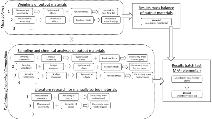
Uncertainties have to be assessed for own measurements and data from literature research. Due to this, an uncertainty propagation with an appropriate mathematical model has to be applied, which provides one value for overall uncertainty (see Figure 3). In this study, measurement uncertainties for weighing the output materials were not considered as systematic and random effects are usually very low for such operations.

Figure 3: Mathematical model for the calculation and uncertainty propagation of an MFA on an elemental basis

Weighing of output materials

Mas s bal anc e Measurement uncertainty Systematical

effects Random effects Measurement

uncertainty

Systematical

effects Random effects

1 2 Uncertainty mass flow [kg] Uncertainty mass flow [kg] 3 …

+

X

Eval uat ion of chem ic al Composi ti on Measurement uncertainty Reliability of source Measurement uncertainty Reliability of source 1 2 3 … Uncertainty mass fraction [ppm] Uncertainty mass fraction [ppm]

Literature research for manually sorted materials

+

Sampling

uncertainty

Systematical

effects Random effects Sampling

uncertainty

Systematical

1 2 3 Uncertainty mass fraction [ppm] Uncertainty mass fraction [ppm]

Sampling and chemical analyses of output materials

+

Analysis inaccuracy Analysis inaccuracy

+

4 … Sampling uncertainty Systematical

Uncertainty mass fraction [ppm] Analysis

inaccuracy

+

Results batch test MFA (elemental)

Uncertainty mass fraction [ppm]

Element Uncertainty loads [kg]

Results mass balance of output materials

Material Uncertainty freights [kg]

(11)

Page 11 of 30

2.4.2. Assessment of systematic effects

In this extended batch test study, systematic effects were identified via (1) redundancy of chemical analyses, (2) a comparison of material and element distribution, (3) case-specific methods, and (4) a comparison of the input-output loads.

(1) Redundancy of chemical analyses

In this extended batch test, up to three different laboratories were assigned to perform the chemical analyses of the output fractions. A comparison of the results revealed systematic effects.

(2) Comparison of material to element distribution

Data from the sorting analyses was used to calculate the expected mass fractions and loads for the elements investigated, along with the literature data for each output fraction in the batch test. The results were then compared directly to the results of the chemical analyses. As only material >5 mm was sorted, additional data from the sieving analyses was used to verify the results. Inconsistent results for single elements had to be checked subsequently with appropriate methodologies like further chemical characterization using other techniques.

(3) Case-specific methods

The chemical analyses of the sample AS1 for the element gold revealed high variances, which were due to systematic effects. Results from the “comparison of material to element distribution” did not clearly verify high gold mass fractions. To avoid misinterpretation, subsequent washing tests were conducted, to investigate the fines in the sample, which were not sorted. For this, three representatively divided samples from the ferrous metals scrap were treated with a 1% and a 2% aqua regia solution over a given period in an overhead shaker at room temperature. After 15, 30 and 60 minutes, samples of the liquid were taken and analyzed for gold with an ICP-AES (Thermo Scientific iCAP 6000 Series).

(4) Comparison of input-output loads

A comparison of input-output loads verifies the MFA model and shows potential systematic effects. In this study, this comparison was carried out using the example of gold, as most analytical problems were related to this element. In order to compare the cumulated loads from the output fractions, an estimate of the gold content in the input material was carried out. PCBs and gold connectors were identified as carriers and corresponding mass shares in the input were approximated based on the results from the input sorting. Oguchi et al., 2011 and Ueberschaar et al., 2017 indicate PCB contents in WEEE devices and related gold mass fractions. For the estimation, we differentiate in two PCB qualities. PCBs in ordinary household devices were calculated conservatively with 100 ppm gold content. Generously equipped PCBs in information and telecommunication equipment such as mobile phones, desktop PCs, notebooks, etc. were conservatively calculated with 500 ppm gold.

Literature research gave an indication of gold loads for connectors. By estimated surface areas covered and a layer thickness of 0,02-0,08 µm Au (Vincenz et al., 2010), the gold loads were assessed. The results of this input estimate were compared with the cumulated gold loads, based on the chemical characterization of the output fractions.

2.4.3. Assessment of random effects

In this study, random effects were determined via (1) calculation of sampling uncertainties, and (2) determination of measurement uncertainties.

(1) Sampling uncertainty

Uncertainties were assessed for all samples taken from the automated sorting processes following Gy, 1992a, 1992b, 1998 and Geelhoed and Glass, 2004. This factor depended on the physical and chemical

(12)

Page 12 of 30

properties and was calculated for each target element. Formula 1 shows the basis for further calculations.

Formula 1: Calculation of the sampling uncertainty following (Francois-Bongarcon and Gy, 2002; Gy, 1998)

𝜎_𝐹𝑆𝐸 =√ 𝑓𝑔(1 − 𝑎_𝑎 𝐿) 𝐿 [(1 − 𝑎𝐿)𝛿𝐴+ 𝑎𝐿𝛿𝐺])𝑑𝑙𝑑 2 𝑀_𝑆 With:

f = shape factor, g = size range parameter, aL = decimal proportion of target component A in lot L, δA = density of target component A, δG = mean density of remaining, non-target component G,

dl = liberation diameter, d = average grain diameter, MS = mass of sample taken [g]

For the assessment of all other necessary parameters, the material was investigated prior to the extended batch test. With this information, a sampling uncertainty was calculated for each output fraction from automated sorting and only for those elements which were listed as target elements for this study and were over the detection limit in the chemical analyses. The supporting information S9 depicts an example calculation for the output fraction AS1 and the sample mass for laboratory 1. (2) Measurement uncertainties

“A random error is associated with the fact that when a measurement is repeated, it will generally provide a measured quantity value that is different from the previous value” (Joint Committee for Guides in Metrology, 2009). Via multiple measurements or a calculated measurement device dependent uncertainties, each laboratory provided a measurement uncertainty for each element analyzed (cf. supporting information S8).

2.4.4. Uncertainties for literature-derived data

External sources always carry particular uncertainties since the data gathering method is frequently not well described and uncertainties not quantified. The use of various methodologies on different sample types by other research teams produces random rather than systematic effects. Following Laner et al., 2015, Table 4 shows the uncertainties according to the data source reliability and the level of specificity used in this study.

Table 4: Uncertainties according to the data source reliability (Laner et al., 2015)

Source / reliability Specificity / representativeness Coefficient of variance [%] National statistical office or independent

institutions Research

National data

Data based on numerous measurements of the quantity of interest

1.5

Official statistics from interest groups/ associations

Research studies

National data

Data based on several measurements of the quantity of interest

4.5

Individual organizations Research studies

Company-specific (fractional) data

Few measurements or measurements not fully representative for the quantity of interest (but transferable)

13.75

Expert estimates Research studies Data based on aggregation of expert estimates Measurements of limited representativeness (unknown transferability)

41.5

(13)

Page 13 of 30

2.5. Calculation of the mass balance

2.5.1. General calculation

The general approach for determining the mass balance on the elemental level is described in Formula 2. Formula 3 shows the calculation of element specific transfer coefficients following Chancerel et al., 2009 and Rotter et al., 2004.

Formula 2: Calculation of mass balance on element level

𝑚_{𝑖,𝑖𝑛𝑝𝑢𝑡}= 𝑚_{𝑖𝑛𝑝𝑢𝑡}∗ 𝑥_{𝑖,𝑖𝑛𝑝𝑢𝑡} = ∑ 𝑚_{𝑖,𝑓𝑟𝑎𝑐𝑡𝑖𝑜𝑛}_𝑗∗ 𝑥_{𝑖,𝑓𝑟𝑎𝑐𝑡𝑖𝑜𝑛}_𝑗

𝑘

𝑗=1

Formula 3: Calculation of element specific transfer coefficients

𝑇𝐶_{𝑖,𝑓𝑟𝑎𝑐𝑡𝑖𝑜𝑛}

𝑗 =

𝑚_{𝑖,𝑓𝑟𝑎𝑐𝑡𝑖𝑜𝑛}_𝑗∗ 𝑥_{𝑖,𝑓𝑟𝑎𝑐𝑡𝑖𝑜𝑛}_𝑗

𝑚𝑖𝑛𝑝𝑢𝑡∗ 𝑥𝑖,𝑖𝑛𝑝𝑢𝑡

With:

x = mass fraction (mg/kg), m = mass (kg); indices: j = output fraction from batch test, i = substance / element, k = number of output fractions

2.5.2. Uncertainty calculation

Due to the methods used for sampling and analysis, only one value is provided by the chemical analyses of the output fractions. The approach used cannot give any insight in the statistical distribution of the sampled output fraction. Following usual practice, we assume a normal distribution (Chancerel et al., 2009; Joint Committee for Guides in Metrology, 2012, 2008; Laner et al., 2014). Therefore, the necessary uncertainty propagation is based on the Gaussian concept. In contrast to the principle of maximum uncertainties, relative uncertainties are calculated for all random effects determined. The uncertainty calculation is performed separately for manually sorted and automatically sorted materials (cf. Formula 4 and Formula 5). Formula 6 describes the calculation of the overall input quantity.

Formula 4: Calculation of uncertainty for manually sorted materials 𝜎_𝑀𝑆 = √𝜎_𝐿𝑆2 + 𝜎_𝐷𝑆𝑅2 Formula 5: Calculation of uncertainty for automatically sorted materials

𝜎_𝐴𝑆= √𝜎_𝐹𝑆𝐸2 _{+ 𝜎} 𝑀𝑈2

Formula 6: Calculation of uncertainty for overall input quantity

𝜎_𝐼𝑄 = √𝜎_𝑀𝑆2 + 𝜎_𝐴𝑆2

With:

σMS = uncertainty for manually sorted materials, σAS = uncertainty for automatically sorted materials, σIQ = uncertainty for the overall input quantity, σLS = uncertainty of data in literature sources (cf. supporting information S7), σDSR = uncertainty according to data source reliability (cf. Table 4), σFSE = sampling uncertainty (cf. Table 5), σMU = measurement uncertainty (cf. supporting information

(14)

Page 14 of 30

This kind of error propagation usually adds a covariance coefficient. The variables are completely independent, which results in a nullification of the correlation and covariance coefficients. Thus, the covariance coefficient was not included.

3. Results

3.1. Uncertainty assessment

3.1.1. Assessment of systematic effects

Comparison of material to element distribution

With the information from the sorting analyses, the results of the chemical analyses could be validated. To this end, mass fractions of target metals in the sorted materials were assumed. The detailed list is attached in the supporting information S13.

For IBMs like Fe and Al, the results were almost in the same range. For substances applied only in low concentrations in the original components or devices, some of the findings from the sorted materials differed substantially from the results of the chemical analyses. This effect was also noticeable for cobalt and REE. Here, a significant share was possibly contributed by magnet material (mostly NdFeB magnets). These components were pulverized during the shredding processes. Occasionally, single clots of magnetic material stuck together with ferrous metals were found in the ferrous metals scrap. A closer examination with an XRF handheld (Thermo Fisher/Analyticon XL3 air) revealed high contents of REE and Co and identified this material partially as NdFeB magnets. As this material was highly contaminated, it was not sorted as a separate material fraction in the sorting analysis carried out. Figure 4 shows the examples aluminum and gold. The results for the other metals investigated are depicted in the supporting information S13.

Figure 4: Comparison of Al content in output materials based on chemical analyses and sorting analyses

0 10 20 30 40 50 60 70 M as s frac ti o n [%] Al sorting analysis Al chemical analysis 0 5 10 15 20 25 30 35 40 45

AS1 AS2 AS3 AS4 AS5

M as s frac ti o n [p p m] Output material Au sorting analysis Au chemical analysis Aluminum Gold

(15)

Page 15 of 30

Due to higher findings using the chemical analyses, trace metals were suspected in the fines of the output fractions, as only material over 5 mm was sorted. This non-sorted material constituted a significant proportion of the total material with a range between 2% and 19% (cf. Figure 8).

Gold analysis

The determination of the element gold was related to high systematic effects. This applied in particular to the sample AS1. Here, laboratory 1 determined mass fractions of about 67 ppm Au. In line with the high masses of this output fraction, the gold load was expected to be extremely high. Further analyses confirmed these high concentrations. A further sample from another test at the same facility had comparable results. As the sorting test showed no corresponding material composition in the form of PCBs, etc., washing tests with subsequent chemical analyses were carried out, to investigate the fines for gold content. Results showed gold mass fractions of from 1x10-3_{to 3x10}-2_{ppm. This did not confirm} the high gold content in the ferrous metals scrap. Subsequently, laboratory 3 (cf. Table 3) developed a specific methodology for reliably determining the gold content of sample AS1. The results revealed an actual gold mass fraction of 0.9 ppm. This results was verified by the comparison of input-output loads. Comparison of input-output loads

Using the example of gold, the input and output loads of the extended batch test were compared. Approximately 210 g gold related to the input of PCBs and ~0.2 g to the gold connectors. From this, a total of 210 g gold was estimated for the input. The calculated gold content in the output is about 240 g. This verified the analytical approach and the data basis of this study.

3.1.2. Assessment of sampling uncertainties

Using Formula 1 as presented above and the sample masses, a sampling uncertainty was calculated for each target element and output fraction of the automated sorting process. Table 5 shows the results. As various sample sizes were used for the analyses, each laboratory refers to different uncertainties. The sampling uncertainties were assessed only for those target elements which were over the detection limit. Therefore, only the S-CRM Co and the REE are depicted.

Table 5: Sampling uncertainties for target elements according to sample size and output fraction

Target material

Responsible laboratory

Sampling uncertainties calculated as %

AS1 AS2 AS3 AS4 AS5 AS6 AS7 AS8

Au, Ag, Pd, Ga Lab 1 2.0 0.4 1.1 0.1 0.6 0.04 0.03 0.04 Lab 2, 3 5.4 - 0.3 1.3 0.2 0.06 - Cu Lab 1 4.1 1.5 1.1 0.4 0.9 0.04 0.05 0.04 Lab 2 11.3 - 0.9 1.9 0.2 0.08 - Fe Lab 1 0.1 0.2 2.4 1.0 3.8 0.04 0.03 0.04 Lab 2 0.2 - 2.5 8.0 0.2 0.06 - Al Lab 1 2.3 0.9 0.2 1.0 1.3 0.04 0.03 0.04 Lab 2 6.4 - 2.5 2.7 0.2 0.06 -

Co, REE Lab 1 9.8 2.0 4.7 8.9 6. 0 0.04 0.03 0.04

Lab 2 26.6 - 22,0 12.7 0.2 0.6 -

According to Francois-Bongarcon and Gy (2002), uncertainties of under 7% are acceptable for a reliable sampling. As depicted, some laboratories were linked to higher uncertainties as they received lower sample quantities for determining particular elements. Results from laboratory 1 were considered to

(16)

Page 16 of 30

be the most accurate. Only for cobalt and REE in AS1 and AS4 were the uncertainties slightly higher than 7%.

3.2. Fate of materials and elements in extended batch test

3.2.1. Calculated element input

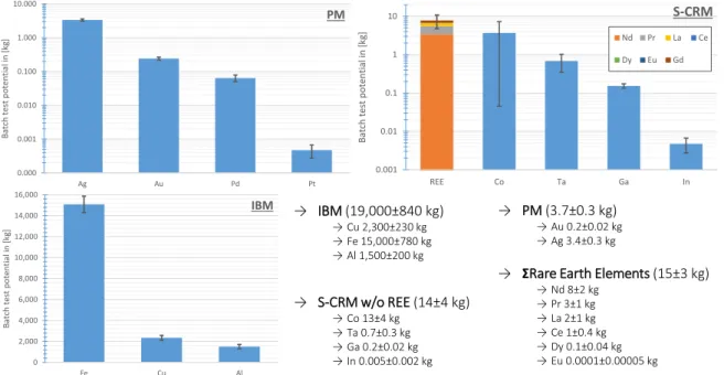
Figure 5 shows the element input calculated in the extended batch test with a total mass of 42,860 kg. The highest share of metals was represented by the IBMs, in particular iron, followed by copper and aluminum. PMs and S-CRMs constituted only a small quantity in the extended batch test. About 4 kg of PMs, mostly silver, were processed. REE and cobalt dominated the S-CRMs.

Figure 5: Calculated material input quantities (errors bars based on all assessed uncertainties)

3.2.1. Distribution of metals in output fractions

With the validated data, not only the general mass flows in the extended batch test, but also the flows of the elements studied, along with corresponding uncertainties, can be presented. The transfer coefficients calculated are a highly important tool for the evaluation of the data generated. Supporting information S12 shows the data in detail. Figure 6 shows the aggregated data on all mass flows. The elemental material flow analysis depicts the elemental distribution of input material to output fractions. The schematic presentation is structured by IBM, PM, and S-CRM. The REE are depicted as a cumulated mass ΣREE.

0.000 0.001 0.010 0.100 1.000 10.000 Ag Au Pd Pt Bat ch t es t p o ten tia l in [ kg] PM → PM (3.7±0.3 kg) →Au 0.2±0.02 kg →Ag 3.4±0.3 kg → IBM (19,000±840 kg) →Cu 2,300±230 kg →Fe 15,000±780 kg →Al 1,500±200 kg → S-CRM w/o REE (14±4 kg) →Co 13±4 kg →Ta 0.7±0.3 kg →Ga 0.2±0.02 kg →In 0.005±0.002 kg

→ ΣRare Earth Elements (15±3 kg)

→Nd 8±2 kg →Pr 3±1 kg →La 2±1 kg →Ce 1±0.4 kg →Dy 0.1±0.04 kg →Eu 0.0001±0.00005 kg 0.001 0.01 0.1 1 10 REE Co Ta Ga In B at ch te st p ot en tial in [ kg] S-CRM Nd Pr La Ce Dy Eu Gd 0 2,000 4,000 6,000 8,000 10,000 12,000 14,000 16,000 Fe Cu Al Bat ch t es t p o ten tia l in [ kg] IBM

(17)

Page 17 of 30

Figure 6: Mass balance and mass flows in extended batch test a) total mass, b) aluminum, copper and iron c) silver, gold, palladium and platinum, d) cobalt, gallium, indium, tantalum and ΣREE

More than one-third of the material was separated manually before mechanical processing. These manual sorting fractions consisted of whole devices like IT devices MS8 (smartphones, tablets, notebooks, etc.) or tools MS1 and single components like drivers from loudspeakers MS3, batteries

(18)

Page 18 of 30

MS7 or power supplies MS4-2. The other two main quantities were ferrous metals scrap AS1 and the sorting residues AS5, which consisted mostly of plastics.

About 47% of aluminum ended up in the non-ferrous scrap AS3, up to 15% in the sorting residues AS5 and 17% in the manually sorted IT devices MS8. Most of the copper was separated manually before mechanical processing, but 20% still ended in the sorting residues AS5. Due to the very efficient magnetic separator, 45% of iron was removed in manual separation, and 65% from the ferrous metals scrap AS1.

PMs like silver were distributed to all output fractions. Most of the significant loads of gold and Pd were separated during the pre-sorting but were distributed to almost all output fractions in the automated sorting. Highest loads were found in manually sorted materials, but also in low magnetic materials AS2 and in particular in the sorting residues AS5.

ΣREE and Cobalt represented the highest share of the S-CRMs. Most of it was concentrated in the pre-sorting step (ΣREE 38%, Co 46%) due to battery removal (MS7). SLF (fluff) AS6 also contained a significant share of Co, at 20%. Over 30% of Co and about 60% of ΣREE was enriched in the ferrous metals scrap AS1.

Figure 7 shows the general splitting of the target metals into manually sorted materials before the mechanical processing and materials from the automated sorting, including the corresponding uncertainties. As described earlier, no uncertainties were assessed for the total mass. These distribution figures relate to the mass fractions in the output investigated and to the transported masses. The mass fractions for the manually sorted materials are shown in the supporting information S7, while the mass fractions for the automated sorted output fractions are depicted in the supporting information S8.

(19)

Page 19 of 30

Figure 7: Splitting of IBM, PM, and S-CRM through manual and automated sorting and distribution in output fractions of automated sorting processes

Except for copper, all elements investigated were mostly concentrated in the automated sorting materials. The main reason for this was the high mass share of about two-thirds that went to the mechanical processing but was also due to the high mass fractions of elements in one of the output fractions.

Depending on the aims of the sorting process, the agglomeration of compatible elements in output fractions is to be desired, but the presence of some other elements can have a contaminating effect on the material. For example, iron was concentrated in the ferrous metals scrap but was related to high loads of Co and ΣREE.

Also noticeable was the high transfer of PMs as well as copper and aluminum to the sorting residues AS5, which consisted mostly of mixed plastics. As in the case of ferrous metal scrap AS1, these sorting residues were significant in quantity and contained a high load of target elements even with low determined mass fractions.

a) D istrib u tio n o f targ et m et als in to m an u al ly (MS) and auto m at e d so rted (AS ) o u tpu t fractio n s b ) D istrib u tio n o f targ et m et als in to au to m ate d so rted (A S) m ateri al s 0 10 20 30 40 50 60 70 80 90 100 Total mass Ag Au Pd Cu Co Al Fe ΣREE Sh are [%] AS1 AS2 AS3 AS4 AS5 AS6 AS7 AS8 0 10 20 30 40 50 60 70 80 90 100 Sh are [%] AS MS

(20)

Page 20 of 30

3.3. Quality assessment of output fractions from pre-processing

3.3.1. Sorting analysis of mechanically processed materials

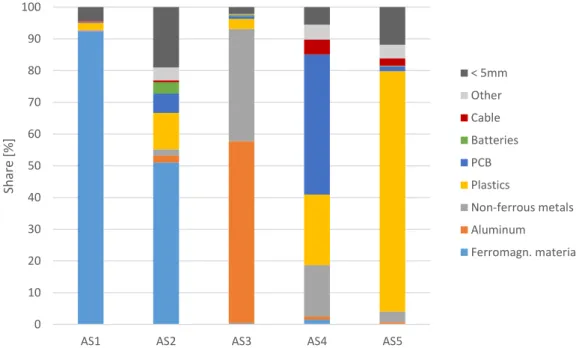
The two plant output fractions ferrous metals scrap (AS1) and non-ferrous scrap (AS3) showed a purity above 92-93% of designated materials, while other output fractions had much higher contaminations from undesignated materials. In particular, in shredded PCBs (AS4) contaminations existed in all grain sizes.

Carriers of target metals like PCBs for PM, tantalum or gallium or batteries for cobalt and REE were found in various output fractions. PCB pieces were dispersed amongst almost all plant output fractions, despite the fact that AS4 and AS2 (low magnetic materials) were the intended routes to ensure the recovery of PMs. Also, 1.5% of the sorting residues AS5 and about 0.8% of AS3 also consisted of these materials. Batteries accounted for a mass share of 3.5% in AS2 (see Figure 8).

Figure 8: Composition of recyclates from mechanical processing based on sorting analysis

3.3.2. Sieve analysis with determination of chemical composition

Results show that the mass fractions of S-CRMs and PMs were partially higher in smaller grain sizes. However, the overall share of fines in output fractions from the automated sorting was usually low, with an average of 8.5% for the samples AS1-5. Exceptions were filter dust and SLF (fluff). IBMs were distributed more evenly in the single sieve ranges. For example, copper was usually evenly concentrated in larger screen sizes. In contrast, the CRMs were located more in the smaller grain sizes. In general, 30-50% of the S-CRMs and up to 90% of the PMs enrich in grain sizes below 5 mm. Figure 9 shows the distribution of Ga, Co, and ΣREE in the output fraction AS4.

0 10 20 30 40 50 60 70 80 90 100

AS1 AS2 AS3 AS4 AS5

Sha re [ % ] < 5mm Other Cable Batteries PCB Plastics Non-ferrous metals Aluminum Ferromagn. material

(21)

Page 21 of 30

Figure 9: Example of sieve analysis of shredded PCBs (AS4) and cumulative masses of Ga, Co, and ΣREE in screening steps The supporting information S11 depicts the results for all other studied output fractions regarding IBMs, PMs, and S-CRMs. Supporting information S10 shows the results of the sieve analysis.

3.4. Identification of hotspots for the recovery of target metals

As shown, target elements were scattered to various output fractions. To assess the potential to separate and recover them, plant output fractions were given an element specific assessment based on their “grade” and the “transfer coefficient” plotted in a hotspot diagram (cf. supporting information S7, S8, and S12).

Figure 10 shows both indicators for cobalt and tantalum. Cobalt was mostly found in magnet materials and batteries, which are applied in various mobile devices. These were manually sorted before the mechanical processing. Also, a single battery fraction (MS7) was separated, representing the major load of cobalt, with almost 35% of total cobalt input and a high mass fraction of over 20,000 ppm. Ferrous metals scrap AS1 was found to hold over 30% of the cobalt load, but with only a minor mass fraction. 0% 10% 20% 30% 40% 50% 60% 70% 80% 90% 100% 0.1 1.0 10.0 100.0

C

u

mmula

tiv

e

mass

(

%

)

Grain diameter (mm)

Ga

Co

Σ

REE

Total

mass PCB

(22)

Page 22 of 30

Figure 10: Hotspot plot for cobalt and tantalum in the output fractions with the highest mass fractions

Most of the tantalum probably derived from alloys and tantalum capacitors used in PCBs. Relevant output materials for tantalum were mainly located in the pre-sorted materials. The highest share of over 40% of the total tantalum loads, with a grade of nearly 1,400 ppm, was accounted for by pre-sorted PCBs (MS5). This might provide a useful basis for the recovery of tantalum in the future. In addition to this output, laptops and desktop PCs also held a significant share of the tantalum loads, with between 25 and 30%. However, the total weight of the laptops and PCs reduced the relative mass fractions. This would appear to be another useful source, but a subsequent separation of the PCB from the device is necessary. This processes did not take place in the plant investigated and is not a part of this study. Other devices like mobile phones, smartphones, and tablets have high mass fractions but were related to low transferred masses due to low collection rates.

Figure 11 shows the hotspot diagram of all REE investigated as a sum and indium. Almost 60% of the total REE were concentrated in the ferrous metals scrap (AS1). This suggests that this output is the most promising regarding the recovery of REE. However, the mass fraction was very low. In contrast, about 30% of the ΣREE was concentrated in the batteries MS7 in the manual sorting step. Here, the mass fractions were much higher. Based on this, batteries would appear to be a significantly better source for the recovery of REE, whereby the set of applied REE differs for NdFeB magnets, batteries or even lighting products (Rotter et al., 2016; Sommer et al., 2015; Ueberschaar and Rotter, 2015). All

0 200 400 600 800 1,000 1,200 1,400 1,600 0 10 20 30 40 50 M ass fractio n o f elem ent [p p m ] Transfer coefficient [%]

Tantalum

Pre-sorted PCB (MS5) Laptops (MS) Tablet (MS) Desktop PC (MS) Scanner (MS) Mobile Phone (MS) Smart Phone (MS) 0 5,000 10,000 15,000 20,000 25,000 30,000 35,000 40,000 45,000 0 10 20 30 40 50 M ass fractio n o f elem ent [p p m ] Transfer coefficient [%]

Cobalt

Laptops (MS) Tablet (MS) Desktop PC (MS) Mobile Phone (MS) Smart Phone (MS) TV TFT (MS) Batteries (MS)

Ferrous metals scrap (AS1) SLF (Fluff) (AS6) 0 5,000 10,000 15,000 20,000 25,000 30,000 35,000 40,000 45,000 0 10 20 30 40 50 M ass fractio n o f elem ent [p p m ] Transfer coefficient [%]

Cobalt

Laptop (MS8-1) Tablet (MS8-2) Desktop PC (MS8-3) Mobile Phone (MS8-6) Smartphone (MS8-7) TV TFT (MS8-8) Batteries (MS7)

Ferrous metals scrap (AS1) SLF (Fluff) (AS6) 0 200 400 600 800 1,000 1,200 1,400 1,600 0 10 20 30 40 50 M ass fractio n o f elem ent [p p m ] Transfer coefficient [%]

Tantalum

Pre-sorted PCB (MS5) Laptop (MS8-1) Tablet (MS8-2) Desktop PC (MS8-3) Scanner (MS8-5) Mobile Phone (MS8-6) Smartphone (MS8-7) 0 5,000 10,000 15,000 20,000 25,000 30,000 35,000 40,000 45,000 0 10 20 30 40 50 M ass fractio n o f elem ent [p p m ] Transfer coefficient [%]

Cobalt

Ferrous metals scrap (AS1) SLF (Fluff) (AS6) 0 200 400 600 800 1,000 1,200 1,400 1,600 0 10 20 30 40 50 M ass fractio n o f elem ent [p p m ] Transfer coefficient [%]

Tantalum

Pre-sorted PCB (MS5) Laptop (MS8-1) Tablet (MS8-2) Desktop PC (MS8-3) Scanner (MS8-5) Mobile Phone (MS8-6) Smartphone (MS8-7)

(23)

Page 23 of 30

other battery containing materials like mobile phones, smartphones and tablets had only low concentrations and held only a small percentage of the total amount of ΣREE.

Figure 11: Hotspot plot for ΣREE and indium in the output fractions with the highest mass fractions

Indium is applied mostly in display devices and was only detected in the manually sorted materials. The various indium mass fractions in the flat screen / TFT displays and the screen dimensions directly influence the indium loads. The highest mass fractions of indium were found in tablets (MS8-2), mobile phones (MS8-6) and smartphones (MS8-7). Due to the low collection rates of these devices and, more specifically, to the low amounts in this batch, the highest indium loads were contributed by laptops. The impact of monitors and TVs was limited.

The distribution figures for PMs (gold, silver), copper and the S-CRM gallium are shown in the supporting information S14. Iron and aluminum were dispersed among all output fractions investigated. A presentation in the same form would not be feasible.

Recycling of the investigated elements from the output fractions generated in the pre-processing of WEEE is not always possible or economically feasible. Therefore, a recyclability assessment for each element and output fraction was carried out. Supporting information S15 presents the results.

0 10 20 30 40 50 60 70 80 90 100 0 20 40 60 80 100 M ass fractio n o f elem ent [p p m ] Transfer coefficient [%]

Indium

Laptops (MS) Tablet (MS) Scanner (MS) Mobile Phone (MS) Smart Phone (MS) TV TFT (MS) Monitor TFT (MS) 0 5,000 10,000 15,000 20,000 25,000 0 20 40 60 80 100 M ass fractio n o f elem ent [p p m ] Transfer coefficient [%]

Σ

Rare Earth Elements

Laptops (MS) Tablet (MS) Desktop PC (MS) Mobile Phone (MS) Smart Phone (MS) Batteries (MS) Ferrous metals scrap (AS1) 0 5,000 10,000 15,000 20,000 25,000 30,000 35,000 40,000 45,000 0 10 20 30 40 50 M ass fractio n o f elem ent [p p m ] Transfer coefficient [%]

Cobalt

Ferrous metals scrap (AS1) SLF (Fluff) (AS6) 0 5,000 10,000 15,000 20,000 25,000 0 20 40 60 80 100 M ass fractio n o f elem ent [p p m ] Transfer coefficient [%]

Σ

Rare Earth Elements

Laptop (MS8-1) Tablet (MS8-2) Desktop PC (MS8-3) Mobile Phone (MS8-6) Smartphone (MS8-7) Batteries (MS7) Ferrous metals scrap (AS1) 0 10 20 30 40 50 60 70 80 90 100 0 20 40 60 80 100 M ass fractio n o f elem ent [p p m ] Transfer coefficient [%]

Indium

Laptop (MS8-1) Tablet (MS8-2) Scanner (MS8-5) Mobile Phone (MS8-6) Smartphone (MS8-7) TV TFT (MS8-8) Monitor TFT (MS8-10) 0 5,000 10,000 15,000 20,000 25,000 0 20 40 60 80 100 M ass fractio n o f elem ent [p p m ] Transfer coefficient [%]

Σ

Rare Earth Elements

Laptop (MS8-1) Tablet (MS8-2) Desktop PC (MS8-3) Mobile Phone (MS8-6) Smartphone (MS8-7) Batteries (MS7) Ferrous metals scrap (AS1) 0 5,000 10,000 15,000 20,000 25,000 0 20 40 60 80 100 M ass fractio n o f elem ent [p p m ] Transfer coefficient [%]

Σ

Rare Earth Elements

Laptop (MS8-1) Tablet (MS8-2) Desktop PC (MS8-3) Mobile Phone (MS8-6) Smartphone (MS8-7) Batteries (MS7) Ferrous metals scrap (AS1)

(24)

Page 24 of 30

4. Discussion

Due to the application of a variety of methodologies summarized to one data set to investigate the flows of particular elements, some approaches have to be discussed.

4.1. Sampling

Taking single samples and cumulating them into one total quantity in order to sample continuous material streams can lead to unexpected failures. The characteristics of the single samples investigated represent only a small share of all the material processed. During sampling breaks, significant variations in the composition and subsequently in the mass fractions measured can take place. This “nugget effect” is a chaotic component and can be considered as the variance of an entirely random component (François-Bongarçon, 1994; Pitard, 1994). Supporting information S16 shows an example of a variation of grain sizes and the mass fraction for one element over time. Depending on the sampling schedule, single extreme variations of the mass fraction can pass undiscovered. This leads to an over- or underestimate of the real value.

An approach with much more statistical power could be premised on a sampling methodology based on many single samples taken randomly over time that are subsequently chemically analyzed. By using a large amount of single values, the variability of each material investigated can be determined (Laner et al., 2014). Related distribution patterns can then be drawn which not only supply information about the expected average values, including uncertainties but also about the variability of the mass flow being studied, minimizing the risk of a nugget effect.

4.1.1. Sampling uncertainty for SLF (fluff)

In this study, Gy’s formula was used to determine sampling uncertainties. This methodology focused initially on compact materials. As the shredder light fractions have a very fluffy appearance with some very long fibers, there were doubts about whether the calculations were suited to this kind of output. Similar application problems are known to have arisen for other formulas in some areas (Abzalov, 2011; Bloch von Blottnitz, 1999; Bunge and Bunge, 1999; Dihalu, 2012). This suggests that a new development or an adaption of a practicable formula is needed to apply calculated sampling uncertainties to such materials as SLF (fluff).

4.1.2. Sampling uncertainty for chemical analyses

The sample masses directly influence the quality of the results. Based on the physical and chemical properties of the material to be analyzed, uncertainty can be calculated. This has been done for all output fractions sampled in this study.

However, the sampling uncertainty for the chemical analyses is not considered. For a wet-chemical digestion and a subsequent chemical analysis, usually a mass between 0.1-1 g is used, as the prepared sample is assumed to be homogenous. An according sampling uncertainty is considered to be low and so was not part of any calculation in this study.

4.2. Chemical characterization

The main focus for the extended batch test described is the chemical characterization of all flows. However, varying results based on random or systematic effects can lead to much higher or lower loads of the element being investigated. This particularly applies to flows with large shares of the total input. Examples in this study are the ferrous metals scrap AS1 and the sorting residues output AS5. Also, the detection limits of measurement devices raise similar problems, as element mass fractions below those limits are not considered mass flows. Consequently, total flows can be systematically underestimated for the overall MFA if this flow is set to zero, or systematically overestimated if the limit of detection (LOD) is considered as the average value. In order to improve the sensitivity of the