A mathematical modeling for the lookback option with jump–diffusion using binomial tree method

(1)

Contents lists available atScienceDirect

Journal of Computational and Applied

Mathematics

journal homepage:www.elsevier.com/locate/cam

A mathematical modeling for the lookback option with jump–diffusion

using binomial tree method

✩

Kwang Ik Kim

a

, Hyun Suk Park

b

, Xiao-song Qian

c,∗

a_{Department of Mathematics, Pohang University of Science and Technology, Pohang, 790-784, Republic of Korea} b_{Department of Finance & Information Statistics, Hallym University, Chuncheon, 200-702, Republic of Korea} c_{School of Mathematical Science, Yangzhou University, Yangzhou 225002, PR China}

a r t i c l e i n f o

Article history:

Received 16 May 2009

Received in revised form 4 May 2011

MSC: 65M12 35R35 45K05 62P05 91B28 Keywords:

Binomial tree method Lookback option Jump–diffusion model Viscosity solution

a b s t r a c t

The binomial tree method (BTM), first proposed by Cox et al. (1979) [4] in diffusion models and extended by Amin (1993) [9] to jump–diffusion models, is one of the most popular approaches to pricing options. In this paper, we present a binomial tree method for lookback options in jump–diffusion models and show its equivalence to certain explicit difference scheme. We also prove the existence and convergence of the optimal exercise boundary in the binomial tree approximation to American lookback options and give the terminal value of the genuine exercise boundary. Further, numerical simulations are performed to illustrate the theoretical results.

1. Introduction

Lookback options are path-dependent options whose payoffs depend on the maximum or the minimum of the underlying asset price during the life of the options. An American lookback call (put) option allows it to be exercised at any time prior to expiry and gives the holder the right to buy (sell) at the historical minimum (maximum) of the underlying stock price on exercising the option.

Suppose there is a financial market with two assets

(

Bt

,

St

)

. The first one is a risk-free asset whose priceBtis governed by the equation dBt

=

rBtdtwhereris the constant positive interest rate, and the other is a risky stock. In a given probability space

(

Ω

,

F

,

P

)

, the stock price evolves according to the stochastic differential equation

dSt

St

=

(µ

−

q

)

dt

+

σ

dWt

+

UdNt (1.1)

where the coefficients

µ,

q

, σ

are positive constants,qis the dividend yield,

(

Wt

)

t≥0is a standard Brownian motion,

(

Nt

)

t≥0

is a Poisson process with constant intensity

λ

, andUis a square integrable random variable taking values in

(

−

1

,

+∞

)

(since the price of a financial asset should be positive).

✩_{This work is supported by the PRC grant NSFC 10801115 and by BSRP through the NRF of Korea (Grant Nos. 2010-0025700 and 2010-0007290).} ∗_{Corresponding author. Tel.: +86 13773526668.}

(2)

Consider a lookback option with life time

[

0

,

T

]

and payoff function

g

(

St

,

At

)

=



St

−

At for lookback call options,

At

−

St for lookback put options, whereAtis the path-dependent variable defined as

At

=



_min

0≤τ≤tSτ for lookback call options, max

0≤τ≤tSτ for lookback put options.

LetV

(

S

,

A

,

t

)

be the lookback option price at timetwith stock priceSand path-dependent variableA.1Because the market here is not complete, we may assume risk neutrality for brevity (see [1,2]). Then we must have

µ

=

r

−

λ

kwherek

=

E

[

U

]

andE

[·]

is the expectation operator over the random variableU(see [3]). Using an argument similar to Pham [3], it can be shown that the European lookback option price solves the following partial integro-differential equation:











LV

(

S

,

A

,

t

)

=

0

,

(

S

,

A

)

∈

D

,

t

∈ [

0

,

T

)

∂

V

∂

A

(

A

,

A

,

t

)

=

0

,

A

∈

(

0

,

∞

),

t

∈ [

0

,

T

)

V

(

S

,

A

,

T

)

=

g

(

S

,

A

), (

S

,

A

)

∈

D

,

(1.2) where LV

=

∂

V

∂

t

+

σ

2 2 S 2

∂

2V

∂

S2

+

(

r

−

q

−

λ

k

)

S

∂

V

∂

S

−

(

r

+

λ)

V

+











λ

∫

∞ −1

V

(

S

(

1

+

y

),

min

{

A

,

S

(

1

+

y

)

}

,

t

)

dN

(

y

),

for lookback call options,

λ

∫

∞

−1

V

(

S

(

1

+

y

),

max

{

A

,

S

(

1

+

y

)

}

,

t

)

dN

(

y

),

for lookback put options,

D

=



{

(

S

,

A

)

:

0

<

A

≤

S

<

∞}

for lookback call options,

{

(

S

,

A

)

:

0

<

S

≤

A

<

∞}

for lookback put options, andN

(

x

)

is the distribution function of the random variableU.

For the American lookback options,(1.2)is replaced by a parabolic variational inequality given by











min

{−

_LV

(

S

,

A

,

t

),

V

(

S

,

A

,

t

)

−

g

(

S

,

A

)

} =

0

, (

S

,

A

)

∈

_D

,

t

∈ [

0

,

T

)

∂

V

∂

A

(

A

,

A

,

t

)

=

0

,

A

∈

(

0

,

∞

),

t

∈ [

0

,

T

)

V

(

S

,

A

,

T

)

=

g

(

S

,

A

), (

S

,

A

)

∈

D

.

(1.3)

The binomial tree method (BTM), first proposed in [4] in diffusion models, is one of the most popular approaches to pricing options in diffusion models. By introducing an additional path-dependent variable to each node, the BTM can be extended to the valuation of lookback option (see [5–7]). To simplify the computation, Cheuck and Vorst [8] proposed an equivalent simple state variable BTM for lookback options in diffusion model. In this paper, we study the BTMs for lookback options in jump–diffusion models. It is well known that jump–diffusion models give a better explanation of sudden changes of stock price than diffusion models. Amin [9] first generalized Cox, Ross and Rubinstein’s BTM to jump–diffusion models for vanilla options. Xu et al. [10] gave an optimal error estimation of European options in Amin’s model. Qian et al. [2] and Kim et al. [11] proved the convergence of BTMs for American options and Asian options in jump–diffusion models. In this paper, following the idea of Amin [9], Jiang et al. [7], Dai [12] and Cheuck et al. [8], we develop a BTM for lookback options in jump–diffusion models and simplify it to one state variable. With numerical analysis and the theory of viscosity solution, we prove the convergence of this algorithm. We also show the existence and convergence of the optimal exercise boundary in the binomial tree approximation to American lookback options and give the terminal value of genuine optimal exercise boundary.

The outline for this paper is as follows. In the next section we construct the BTM for lookback options in jump–diffusion models and simplify it to single state variable. In Section3, the equivalence of the BTM and the explicit difference scheme is established. In Section4, we prove the convergence of the BTM. Section5is devoted to showing the existence and convergence of approximate optimal exercise boundary for American lookback options. Finally numerical illustrations are given in Section6to demonstrate the theoretical results provided in the previous sections. Throughout this paper, we will concentrate on lookback call options. The case of lookback put option is similar.

1 Usually we have the lookback option priceVt =V(St,At,t). But when using PDE’s method to price lookback options, we treatS,A,tas independent variables and haveVt=V(S,A,t), just like the case in the well-known Black–Scholes model.

(3)

2. Binomial tree method

In this section, we develop the BTM for lookback options in a jump–diffusion model. The idea stems from Amin [9]. In our discrete time market, trade occurs only on discrete dates in the interval

[

0

,

T

]

. LetZ

= {

0

,

±

1

,

±

2

, . . .

}

,

Nbe the number of discrete time points,1t

=

T

N andti

=

i1tfori

=

0

,

1

,

2

, . . . ,

N. We assume that only two assets are traded in the market. The first is a bondBwhich has a riskless rate of return of

ρ

=

er1t _{in every period. The second asset is a risky stock. We} assume that the underlying stock priceScan take on values in a discrete set

{

ul

:

l

∈

Z

}

withu

=

eσ

√

1t_{. We also assume} that this stock pays a dividend

η

=

eq1t_{for positive constant dividend yield}_q_{in each period.}

We now describe the stock price dynamics. In each period, the stock price undergoes either of the two different types of price changes. In most periods, the stock price undergoes only ‘‘local’’ changes. Analogous to Cox et al.’s BTM [4], the stock priceSmoves up toSuor down toSu−1_{. This price change is the discrete counterpart of the stock price changes due to the}

diffusion component in the continuous time case.

The stock price can be also changed due to the occurrence of a ‘‘rare event’’, which has a low probability of occurring in any given period. It corresponds to the arrival of important information which causes a large change in the stock price. When the ‘‘rare event’’ occurs, the stock price ‘‘jumps’’ to potentially any stateSul

(

l

∈

Z

)

at the next date. But we may assume that the two different kinds of changes in stock price are mutually exclusive, i.e., the stock price cannot ‘‘jump’’ to the adjacent statesSu±1_{. However, in the limit as}_N

_{→ ∞}

_{, it does not matter whether we define the ‘‘jump’’ event in an adjacent state}

or over every point in the state space. LetVn

₍

_S

n

,

An

)

be the option price of lookback call options at timetnwith stock priceSnand path-dependent variableAn. Here we have

An

=

min

0≤i≤nSi

,

whereSi stands for the stock price of such a path at timeti

,

i

=

0

,

1

, . . . ,

n. If at timetn+1, stock priceSnchanges to

Snul

(

l

∈

Z

),

Anwill consequently becomeAln+1, where Al_n+₁

=

min

{

An

,

Snul

}

.

At timetn, we consider a portfolio with one option,∆shares of stock andBdollars in the riskless bond. If we assume that the initial investment in this portfolio at timetnis zero, then the portfolio valueΠnis given by

Πn

₌

₁_S

n

+

B

+

Vn

(

Sn

,

An

)

=

0

.

(2.1)

Suppose the investor wishes to eliminate the risk of this portfolio due to the local changes of stock price in the interval

[

tn

,

tn+1

]

. Then the portfolio value must be equal (not necessarily zero) in the both adjoint statesSnu±1at timetn+1. This

implies that Πn+1 ±1

=

1Snu

η

+

ρ

B

+

Vn+1

(

Snu

,

A+n+11

)

=

1Snu −1

_η

₊

_ρ

B

+

Vn+1

(

Snu −1

_,

A−_n+1₁

).

(2.2)

Solving the above equation for∆yields ∆

= −

V

n+1

₍

_S

nu

,

A+n+11

)

−

Vn+1

(

Snu−1

,

A−n+11

)

Sn

η(

u

−

u−1

)

.

(2.3) Now, eliminating∆andBfrom(2.2)by using(2.1)and(2.3), we obtain

Πn+1 ±1

= ˜

pV n+1

₍

_S nu

,

A+n+11

)

+

(

1

− ˜

p

)

V n+1

₍

_S nu−1

,

A−n+11

)

−

ρ

V n

₍

_S n

,

An

),

(2.4) where

˜

p

=

ρ/η

−

u −1 u

−

u−1

.

(2.5)

Therefore, if there is no jump (‘‘rare event’’), the portfolio is riskless and the expression(2.4)must be equal to zero, which is the BTM for lookback options in diffusion models.

Now, consider the portfolio value when a rare event occurs. LetUbe the relative amplitude of jump on the stock when the rare event occurs andybe the index of the state induced by the jump at the next date. In other words, if the stock price at timetnisSnand a rare event occurs, the stock price at timetn+1will be equal toSn

(

1

+

U

)

=

Snuy. Then the portfolio valueΠn+1

y can be written as Πn+1

(4)

Eliminating∆andBfrom(2.6)by using(2.1)and(2.3), we get Πn+1 y

= −

Vn+1

₍

_S nu

,

A+n+11

)

−

Vn+1

(

Snu−1

,

A−n+11

)

u

−

u−1



U

+

1

−

ρ

η



+

Vn+1

(

Snuy

,

Ayn+1

)

−

ρ

V n

₍

_S n

,

An

).

(2.7)

Analogous to Merton [13] and Amin [9], we assume that the jump risk is diversifiable, which implies that the expectation of the portfolio value in the next period with respect to the distribution of the rare event must be zero. Let the probability of a rare event in time interval1tbe equal to

_λ

ˆ

_{(corresponding to the Poisson jump component of the continuous time process}

in(1.1), we have

λ

ˆ

=

λ

e−λ1t₁_t

₌

_λ

₁_t

₊

_O

₍

₁_t2

₎

_{). Let}_E

U

[·]

be the expectation operator with respect to the distribution ofU. Taking the expectation of the portfolio value at timetn+1with respect to the jump distribution and equating it to zero

yields

0

=

EU

[

Πn+1

] = ˆ

λ

EU

[

Πyn+1

] +

(

1

− ˆ

λ)

Π n+1

±1

.

(2.8)

Substituting the portfolio values from(2.4)and(2.7)for those in(2.8)yields

ρ

Vn

(

Sn

,

An

)

= ˆ

λ



EU

[

Vn+1

(

Snuy

,

Ayn+1

)

] −

Vn+1

(

Snu

,

A +1 n+1

)

−

V n+1

₍

_S nu−1

,

A −1 n+1

)

u

−

u−1



EU

[

U

] +

1

−

ρ

η





+

(

1

− ˆ

λ)

[˜

pVn+1

(

Snu

,

A+n+11

)

+

(

1

− ˜

p

)

V n+1

₍

_S nu−1

,

A−n+11

)

]

.

(2.9)

Further, replacingp

˜

in(2.9)by(2.5), we have

ρ

Vn

(

Sn

,

An

)

=

(

1

− ˆ

λ)

[

pVn+1

(

Snu

,

A+n+11

)

+

(

1

−

p

)

V n+1

₍

_S nu−1

,

A−n+11

)

] + ˆ

λ

EU

[

Vn+1

(

Snuy

,

Ayn+1

)

]

,

(2.10) where p

=

ρ/η− ˆλ(EU[U]+1) 1− ˆλ

−

u −1 u

−

u−1

.

(2.11)

Let the cumulative function ofUbe given byN

(

x

)

forx

>

−

1 (noting thatk

=

EU

[

U

] =



+∞

−1 xdN

(

x

)

), andp

ˆ

l

(

l

∈

Z

)

represent the discrete probability distribution. Then, we have

ˆ

pl

=

Prob



ln

(

1

+

U

)

∈

[

l

−

1 2



σ

√

1t

,



l

+

1 2



σ

√

1t



=

N



e  l+1₂  σ√1t

−

1



−

N



e  l−1₂  σ√1t

−

1



(2.12) and EU

[

Vn+1

(

Snuy

,

Ayn+1

)

] =

−

l∈Z Vn+1

(

Snul

,

Aln+1

)

p

ˆ

l

.

(2.13)

Hence, from(2.10)–(2.13), we obtain the BTM for European lookback options as follows:











Vn

(

Sn

,

An

)

=

1

ρ



(

1

− ˆ

λ)



pVn+1

(

Snu

,

A+n+11

)

+

(

1

−

p

)

V n+1

₍

_S nu−1

,

A−n+11

)



+ ˆ

λ

−

l∈Z Vn+1

(

Snul

,

Aln+1

)

p

ˆ

l



,

VN

(

SN

,

AN

)

=

SN

−

AN

.

(2.14)

It is well known that the BTMs for lookback options, even in diffusion models, would lead to large amount of computation due to the path-dependent variable. Fortunately, Cheuck et al. [8] proposed equivalent but simple single state variable approaches for lookback option in diffusion models. We will show that Cheuck et al.’s technique also works in jump–diffusion models. Define

j

=

ln

(

Sn

/

An

)

lnu

.

(2.15)

SinceAnis a minimum overSiwithi

=

0

,

1

, . . . ,

n, it follows thatjis a non-negative integer indicating the difference in powers ofu, between the actual and the lowest stock price till timetn.

We claim thatVn

(

Sn

,

An

)

is equal toSnmultiplied by a function

v

, which depends onjand actual timetnonly, i.e.,

(5)

where

v(

j

,

tn

)

is defined as follows:











v(

j

,

tn

)

=

1

ρ



(

1

− ˆ

λ)

[

pu

v(

j

+

1

,

tn+1

)

+

(

1

−

p

)

u−1

v(

j

−

1

,

tn+1

)

]

+ ˆ

λ

+∞

−

l=−j+1 ul

v(

j

+

l

,

tn+1

)

p

ˆ

l

+ ˆ

λ

−j

−

l=−∞ ul

v(

0

,

tn+1

)

p

ˆ

l



,

j

≥

1

,

v(

0

,

tn

)

=

1

ρ



(

1

− ˆ

λ)

[

pu

v(

1

,

tn+1

)

+

(

1

−

p

)

u−1

v(

0

,

tn+1

)

]

+ ˆ

λ

+∞

−

l=1 ul

v(

l

,

tn+1

)

p

ˆ

l

+ ˆ

λ

0

−

l=−∞ ul

v(

0

,

tn+1

)

p

ˆ

l



,

v(

j

,

tN

)

=

1

−

u−j

,

j

≥

0

.

(2.17)

This claim is proved by backward induction and follows in due course. As

VN

(

SN

,

AN

)

=

SN

−

AN

=

SN

(

1

−

u−j

)

=

SN

v(

j

,

tN

),

our claim holds for the maturity date.

Consider the point

(

j

,

tn

)

with stock priceSnand path-dependent variableAn. After a small time interval1t, stock price will beSnul

(

l

∈

Z

)

, and path-dependent variable will be

Al_n+₁

=

min

{

An

,

Snul

} =



An

,

j

+

l

>

0

,

Snul

,

j

+

l

≤

0

.

(2.18)

Suppose our claim is true at timetn+1. Then the option price at timetn+1will change to

Vn+1

(

Snul

,

Aln+1

)

=



Snul

v(

j

+

l

,

tn+1

),

j

+

l

>

0

,

Snul

v(

0

,

tn+1

),

j

+

l

≤

0

.

Whenj

≥

1, it follows from(2.14)that

Vn

(

Sn

,

An

)

=

1

ρ



(

1

− ˆ

λ)

[

pSnu

v(

j

+

1

,

tn+1

)

+

(

1

−

p

)

Snu−1

v(

j

−

1

,

tn+1

)

]

+ ˆ

λ

+∞

−

l=−j+1 Snul

v(

j

+

l

,

tn+1

)

p

ˆ

l

+ ˆ

λ

−j

−

l=−∞ Snul

v(

0

,

tn+1

)

p

ˆ

l



=

Sn

v(

j

,

tn

).

Then our claim at timetnis proved.

The claim forj

=

0 can be proved similarly.

Hence, to determine the option price we only have to find the function

v

. Since

v

depends on one state variablejand the time variable, we have constructed a simple binomial model for European lookback options.

For American lookback options, the investor can choose to exercise the options if the current payoff of the options is worth more than its value being held till the next period. Thus, the BTM for American lookback options can be written instead of(2.14)as follows:











Vn

(

Sn

,

An

)

=

max



1

ρ



(

1

− ˆ

λ)



pVn+1

(

Snu

,

A+n+11

)

+

(

1

−

p

)

V n+1

₍

_S nu−1

,

A−n+11

)



+ ˆ

λ

−

l∈Z Vn+1

(

Snul

,

Aln+1

)

p

ˆ

l



,

Sn

−

An



,

VN

(

SN

,

AN

)

=

SN

−

AN

.

(2.19)

(6)

Using the same transformation(2.15)and(2.16), we can similarly obtain the one state variable binomial tree method for American lookback call options as follows:











v(

j

,

tn

)

=

max



1

ρ



(

1

− ˆ

λ)

[

pu

v(

j

+

1

,

tn+1

)

+

(

1

−

p

)

u−1

v(

j

−

1

,

tn+1

)

]

+ ˆ

λ

+∞

−

l=−j+1 ul

v(

j

+

l

,

tn+1

)

p

ˆ

l

+ ˆ

λ

−j

−

l=−∞ ul

v(

0

,

tn+1

)

p

ˆ

l



,

1

−

u−j



,

j

≥

1

,

v(

0

,

tn

)

=

1

ρ



(

1

− ˆ

λ)

[

pu

v(

1

,

tn+1

)

+

(

1

−

p

)

u−1

v(

0

,

tn+1

)

]

+ ˆ

λ

+∞

−

l=1 ul

v(

l

,

tn+1

)

p

ˆ

l

+ ˆ

λ

0

−

l=−∞ ul

v(

0

,

tn+1

)

p

ˆ

l



,

v(

j

,

tN

)

=

1

−

u−j

,

j

≥

0

.

(2.20)

3. Finite difference method

In this section, we establish the relationship between the BTMs and finite difference methods for lookback options in jump–diffusion models. From now on we will concentrate on the American lookback options since it is similar for the European cases.

First we will show that the governing equation of American lookback call options can be simplified under appropriate transformations. Let

x

=

lnS

A

,

v(

x

,

t

)

=

V

(

S

,

A

,

t

)

S

.

(3.1)

Then Eq.(1.3)is reduced to











min



−

L′

v(

x

,

t

), v(

x

,

t

)

−

(

1

−

e−x

)



=

0

,

x

∈ [

0

,

+∞

),

t

∈ [

0

,

T

)

∂v

∂

x

(

0

,

t

)

=

0

,

t

∈ [

0

,

T

)

v(

x

,

T

)

=

1

−

e−x

,

x

∈ [

0

,

+∞

)

(3.2)

whereL′_{is the operator} L′

v

=

∂v

∂

t

+

1 2

σ

2

∂

2

_v

∂

x2

+



r

−

q

−

λ

k

+

σ

2 2



∂v

∂

x

−

(

q

+

λ

+

λ

k

)v

+

λ

∫

+∞ −1

(

1

+

y

)v((

x

+

ln

(

1

+

y

))

+

,

t

)

dN

(

y

).

We now present an explicit finite difference scheme for(3.2). Given mesh size1x

,

1t

,

N1t

=

T, letQh

= {

(

n1t

,

j1x

)

:

0

≤

n

≤

N

,

j

∈

Z

}

stand for the set of lattices,

v

n_j represent the value of numerical approximation of

v(

x

,

t

)

at

(

n1t

,

j1x

)

∈

Qh. Note that the integral term in operatorL′

v

can be changed to the following form

λ

∫

+∞ −1

(

1

+

y

)v((

x

+

ln

(

1

+

y

))

+

,

t

)

dN

(

y

)

=

λ

∫

+∞ −∞ ez

v((

x

+

z

)

+

,

t

)

dN

(

ez

−

1

)

=

λ

∫

+∞ −x ez

v(

x

+

z

,

t

)

dN

(

ez

−

1

)

+

λ

∫

−x −∞ ez

v(

0

,

t

)

dN

(

ez

−

1

).

Then, taking the explicit difference scheme of(3.2), we have forj

≥

0

min



−

v

n+1 j

−

v

jn 1t

−

σ

2 2

v

n+1 j+1

−

2

v

n+1 j

+

v

n+1 j−1 1x2

−



r

−

q

−

λ

k

+

σ

2 2



v

n+1 j+1

−

v

n+1 j−1 21x

+

(

q

+

λ

+

λ

k

)v

_jn

−

λ

+∞

−

l=−j+1 el1x

v

_j+ln+1pl

−

λ

−j

−

l=−∞ el1x

v

n+₀ 1pl

, v

jn

−

(

1

−

e −j1x

₎



=

0

,

(7)

or

v

n j

=

max



1 1

+

(

q

+

λ

+

λ

k

)

1t





1

−

σ

2₁_t 1x2



v

n+1 j

+



σ

2₁_t 21x2

+



r

−

q

−

λ

k

+

σ

2 2



1 t 21x



v

n+1 j+1

+



σ

2₁_t 21x2

−



r

−

q

−

λ

k

+

σ

2 2



1 t 21x



v

n+1 j−1

+

λ

1t +∞

−

l=−j+1 el1x

v

_j+ln+1pl

+

λ

1t −j

−

l=−∞ el1x

v

₀n+1pl



,

1

−

e−j1x



(3.3) where pl

=

N



e  l+1₂  1x

−

1



−

N



e  l−1₂  1x

−

1



.

(3.4) Ifσ21t

1x2

=

1, we conclude from(2.12),(3.3)and(3.4)that

pl

= ˆ

pl (3.5) and

v

n j

=

max



1 1

+

(

q

+

λ

+

λ

k

)

1t



1 2

+



r

−

q

−

λ

k

+

σ

2 2



√

1t 2

σ



v

n+1 j+1

+



1 2

−



r

−

q

−

λ

k

+

σ

2 2



√

1t 2

σ



v

n+1 j−1

+

λ

1t +∞

−

l=−j+1 el1x

v

_j+ln+1pl

+

λ

1t −j

−

l=−∞ el1x

v

₀n+1pl



,

1

−

e−j1x



.

(3.6) In order to approximate boundary∂v_∂_x

(

0

,

t

)

=

0, we let

v

n+1

−1

=

v

n+1 0

.

Then we obtain the following explicit difference scheme











v

n j

=

max



1 1

+

(

q

+

λ

+

λ

k

)

1t



1 2

+



r

−

q

−

λ

k

+

σ

2 2



√

1 t 2

σ



v

n+1 j+1

+



1 2

−



r

−

q

−

λ

k

+

σ

2 2



√

1 t 2

σ



v

n+1 j−1

+

λ

1t +∞

−

l=−j+1 el1x

v

_j+ln+1pl

+

λ

1t −j

−

l=−∞ el1x

v

n+₀ 1pl



,

1

−

e−j1x



,

j

≥

1

v

n 0

=

1 1

+

(

q

+

λ

+

λ

k

)

1t



1 2

+



r

−

q

−

λ

k

+

σ

2 2



√

1t 2

σ



v

n+1 1

+



1 2

−



r

−

q

−

λ

k

+

σ

2 2



√

1t 2

σ



v

n+1 0

+

λ

1t +∞

−

l=1 el1x

v

_ln+1pl

+

λ

1t 0

−

l=−∞ el1x

v

₀n+1pl



v

N j

=

1

−

e −j1x

_,

_j

_≥

₀

_.

(3.7) Notingu

=

eσ √

1t

_{, ρ}

₌

_er1t

_{, η}

₌

_eq1t_{, and}

_λ

ˆ

=

λ

1t

+

O

(

1t2

₎

_{, we can easily verify that}

p

=

1 2

+



r

−

q

−

λ

k

−

σ

2 2



√

1t 2

σ

+

O

(

1t 3 2

)

1

ρ

(

1

− ˆ

λ)

pu

=

1 1

+

(

q

+

λ

+

λ

k

)

1t



1 2

+



r

−

q

−

λ

k

+

σ

2 2



√

1t 2

σ



+

O

(

1t32

),

1

ρ

(

1

− ˆ

λ)(

1

−

p

)

u −1

₌

1 1

+

(

q

+

λ

+

λ

k

)

1t



1 2

−

(

r

−

q

−

λ

k

+

σ

2 2

)

√

1t 2

σ



+

O

(

1t32

).

Comparing(2.20)with(3.7), we deduce the following result:

Theorem 3.1. The binomial tree method(2.20)is equivalent to the explicit difference scheme(3.7)with σ21t

1x2

=

1in the sense

(8)

4. Convergence

In this section, we describe the convergence of BTM for American lookback options. Without loss of generality, we assume that

0

<

p

<

1 (4.1)

which always holds for1tsmall enough. We also assume thatσ₁21t

x2

=

1, then we have

u

=

eσ √

1t

₌

_e1x

_.

_(4.2)

In addition, we will letq

>

0 because whenq

=

0, an American lookback option is reduced to an European one. Because of the equivalence between the BTM(2.20)and the explicit difference scheme(3.7), to simplify notation, we denote

v

n

j

=

v(

j

,

tn

)

(4.3)

from now on. Now we investigate the properties of the BTM(2.20).

Lemma 4.1. The BTM(2.20)has the following properties:

(1)

v

_jn

≤

v

_j+n₁for all n

,

j

≥

0.

(2)

v

_jn+1

≤

v

n

j for all n

,

j

≥

0. (3)

v

n

j

≤

1for all n

,

j

≥

0.

(4)

v

_jn

−

v

_in

≤

u−i

−

u−jfor all n

,

j

≥

i

≥

0.

Proof. We use the induction to prove the properties.

(1) Clearly,

v

N_j

=

1

−

u−j

≤

1

−

u−(j+1)

=

v

N_j+₁. If

v

m+_j 1

≤

v

_j+m+₁1for allj

≥

0, then

v

m j

=

max



1

ρ



(

1

− ˆ

λ)

[

pu

v

_j+m+₁1

+

(

1

−

p

)

u−1

v

m+_j−₁1

] + ˆ

λ

+∞

−

l=−j+1 ul

v

_j+lm+1pl

+ ˆ

λ

−j

−

l=−∞ ul

v

m+₀ 1pl



,

1

−

u−j



≤

max



1

ρ



(

1

− ˆ

λ)

[

pu

v

m+_j+₂1

+

(

1

−

p

)

u−1

v

_jm+1

] + ˆ

λ

+∞

−

l=−j+1 ul

v

_j+l+m+1₁pl

+ ˆ

λ

u−j

v

₁m+1p−j

+ ˆ

λ

−j−1

−

l=−∞ ul

v

m+₀ 1pl



,

1

−

u−j



=

max



1

ρ



(

1

− ˆ

λ)

[

pu

v

₍m+_j+₁1₎₊₁

+

(

1

−

p

)

u−1

v

m+₍_j+₁1₎₋₁

] + ˆ

λ

+∞

−

l=−j ul

v

m+₍_j+₁1₎_+lpl

+ ˆ

λ

−(j+1)

−

l=−∞ ul

v

₀m+1pl



,

1

−

u−j



=

v

_j+m₁ forj

≥

1

,

and the case ofj

=

0 is analogous. (2) By(2.20),

v

_jN−1

≥

1

−

u−j

₌

_v

N

j. If

v

m+1

j

≥

v

m+2

j for allj

≥

0, then

v

m j

=

max



1

ρ



(

1

− ˆ

λ)

[

pu

v

_j+m+₁1

+

(

1

−

p

)

u−1

v

m+_j−₁1

] + ˆ

λ

+∞

−

l=−j+1 ul

v

_j+lm+1pl

+ ˆ

λ

−j

−

l=−∞ ul

v

m+₀ 1pl



,

1

−

u−j



≥

max



1

ρ



(

1

− ˆ

λ)

[

pu

v

_j+m+₁2

+

(

1

−

p

)

u−1

v

m+_j−₁2

] + ˆ

λ

+∞

−

l=−j+1 ul

v

_j+lm+2pl

+ ˆ

λ

−j

−

l=−∞ ul

v

m+₀ 2pl



,

1

−

u−j



=

v

_jm+1 forj

≥

0

,

which is the desired result. (3) Let

v

m_denote

_{

_v

m

j

}

j≥0. We introduce a norm

‖ · ‖

as follows:

‖

v

m

‖ =

sup j≥0

|

v

_jm

|

.

It suffices to show that

‖

v

m

‖ ≤

1 for allm. Clearly,

‖

v

N

‖ =

sup_j≥₀

(

1

−

u−j

)

=

1. If

‖

v

m+1

‖ ≤

1, then forj

≥

1,

v

m j

=

max



1

ρ



(

1

− ˆ

λ)

[

pu

v

_j+m+₁1

+

(

1

−

p

)

u−1

v

m+_j−₁1

] + ˆ

λ

+∞

−

l=−j+1 ul

v

_j+lm+1pl

+ ˆ

λ

−j

−

l=−∞ ul

v

m+₀ 1pl



,

1

−

u−j



≤

max



1

ρ



(

1

− ˆ

λ)(

pu

+

(

1

−

p

)

u−1

)

+ ˆ

λ

−

l∈Z ulpl



,

1

−

u−j



.

(9)

Noting that pu

+

(

1

−

p

)

u−1

=

e (r−q)1t

_{− ˆ}

_λ(

₁

₊

_k

₎

1

− ˆ

λ

(4.4) and

−

l∈Z ulpl

=

∫

+∞ −∞ eydN

(

ey

−

1

)

+

O

(

1t12

)

=

1

+

k

+

O

(

1t12

),

_(4.5) we have

v

m j

≤

max

{

e −q1t

₊

_O

₍

₁_t₂3

_),

₁

₋

_u−j

_{} ≤}

₁

_.

Forj

=

0, we can similarly derive

v

m

0

≤

1. So property (3) is proved.

(4) For all 0

≤

i

≤

j

, v

_jN

−

v

_iN

=

(

1

−

u−j

₎

₋

₍

₁

₋

_u−i

₎

₌

_u−i

₋

_u−j_{. Suppose}

_v

m+1

j

−

v

m+1

i

≤

u−i

−

u−jfor all 0

≤

i

≤

j. To simplify writing, we set

I_jm

=

1

ρ



(

1

− ˆ

λ)

[

pu

v

_j+m₁

+

(

1

−

p

)

u−1

v

_j−m₁

] + ˆ

λ

+∞

−

l=−j+1 ul

v

m_j+lpl

+ ˆ

λ

−j

−

l=−∞ ul

v

₀mpl



.

(4.6) Then I_jm+1

−

I_im+1

=

1

ρ



(

1

− ˆ

λ)

[

pu

(v

_j+m+₁1

−

v

_i+m+₁1

)

+

(

1

−

p

)

u−1

(v

_j−m+₁1

−

v

m+_i−₁1

)

]

+ ˆ

λ

+∞

−

l=−i+1 ul

(v

m+_j+l1

−

v

_i+lm+1

)

pl

+ ˆ

λ

−i

−

l=−j ul

(v

m+_j+l1

−

v

m+₀ 1

)



≤

1

ρ



(

1

− ˆ

λ)

[

pu

(

u−(i+1)

−

u−(j+1)

)

+

(

1

−

p

)

u−1

(

u−(i−1)

−

u−(j−1)

)

]

+ ˆ

λ

+∞

−

l=−i+1 ul

(

u−(i+l)

−

u−(j+l)

)

pl

+ ˆ

λ

−i

−

l=−j ul

(

1

−

u−(j+l)

)

pl



=

1

ρ



(

1

− ˆ

λ)(

u−i

−

u−j

)

+ ˆ

λ

+∞

−

l=−i+1

(

u−i

−

u−j

)

pl

+ ˆ

λ

−i

−

l=−j

(

ul

−

u−j

)

pl



≤

1

ρ



(

1

− ˆ

λ)(

u−i

−

u−j

)

+ ˆ

λ

+∞

−

l=−i+1

(

u−i

−

u−j

)

pl

+ ˆ

λ

−i

−

l=−j

(

u−i

−

u−j

)

pl



≤

1

ρ

(

u−i

−

u−j

)

≤

u−i

−

u−j for all 0

≤

i

≤

j

.

(4.7)

So we have

v

m j

−

v

m i

=











I_jm+1

−

I_im+1 ifI_jm+1

≥

1

−

u−jandI_im+1

≥

1

−

u−i

−

u−j ifI_jm+1

≤

1

−

u−jandI_im+1

≤

1

−

u−i

I_jm+1

−

(

1

−

u−j

)

≤

I_jm+1

−

I_im+1 ifI_jm+1

≥

1

−

u−jandI_im+1

≤

1

−

u−i

(

1

−

u−j

)

−

I_im+1

≤

u−i

−

u−j ifI_jm+1

≤

1

−

u−jandI_im+1

≥

1

−

u−i

.

In all the cases we can deduce from(4.7)that

v

m

j

−

v

m i

≤

u

−i

₋

_u−j _{for all 0}

_≤

_i

_≤

_j

_,

which is the desired result. The proof is completed.

Employing the notion of viscosity solution, we will show the convergence of the BTM for some American lookback options. Firstly, we recall the definition of viscosity solution and it is convenient to have the following notations.

USC

(

R+

× [

0

,

T

]

)

= {

upper semicontinuous functionsu

: [

0

,

+∞

)

× [

0

,

T

] →

R

}

,

(10)

Definition 4.2. A locally bounded functionu

∈

USC

(

R+

_{× [}

0

,

T

]

)

(resp.u

∈

LSC

(

R+

_{× [}

0

,

T

]

)

) is a viscosity subsolution (resp. supersolution) of(3.2)if, for allx

∈

R+

_,

_u

₍

_x

_,

_T

₎

_≤

₁

₋

_e−x_(resp._u

₍

_x

_,

_T

₎

_≥

₁

₋

_e−x_{) and, for all}

₍

_x

_,

_t

₎

_∈

_R+

_{× [}

₀

_,

_T

_{), φ}

_∈

C2

₍

_R+

_{× [}

₀

_,

_T

_]

₎

_{such that}_u

₍

_x

_,

_t

₎

₌

_φ(

_x

_,

_t

₎

_{, and}_u

_{< φ}

_(resp._u

_{> φ}

_{) on}_R+

_×

₍

₀

_,

_T

_]

_/(

_x

_,

_t

₎

_{, we have} min

{−

L′

φ(

x

,

t

), φ(

x

,

t

)

−

(

1

−

e−x

)

} ≤

0

(

resp.

≥

0

)

for

(

x

,

t

)

∈

R+

× [

0

,

T

)

and min



min

{−

L′

φ(

x

,

t

), φ(

x

,

t

)

−

(

1

−

e−x

)

}

,

∂φ

∂

x



≤

0 for

(

x

,

t

)

∈ {

0

} × [

0

,

T

)



resp. max



min

{−

L′

φ(

x

,

t

), φ(

x

,

t

)

−

(

1

−

e−x

)

}

,

∂φ

∂

x



≥

0 for

(

x

,

t

)

∈ {

0

} × [

0

,

T

)



.

Further, we callu

∈

C

(

R+

_{× [}

₀

_,

_T

_]

₎

_{a viscosity solution of}_(3.2)_{if it is simultaneously a subsolution and a supersolution.} The proof for convergence needs the strong comparison principle which holds for(3.2)(see [14–16] and the references therein).

Lemma 4.3 (Comparison Principle).Suppose u and

v

are, respectively, viscosity subsolution and supersolution of problem(3.2), then u

≤

v

.

Remark 4.4. FromLemma 4.3, the uniqueness of the solution for(3.2)follows immediately.

Let

v

_jnbe the function defined by the BTM(2.20). We now define the extension function

v

₁t

(

x

,

t

)

as follows:

v

1t

(

x

,

t

)

=

v

jn forx

∈

[

j

−

1 2



1x

, (

j

+

1 2

)

1x



,

t

∈





n

−

1 2



1t

,



n

+

1 2



1t



.

ByLemma 4.1, we have 0

≤

v

₁_t

(

x

,

t

)

≤

1 (4.8) for small1t.

Theorem 4.5. Suppose that

v(

x

,

t

)

is the viscosity solution of (3.2)for American lookback options. Then, as1t

→

0, we have

v

1t

(

x

,

t

)

converges uniformly to

v(

x

,

t

)

in any bounded closed subdomain ofR+

× [

0

,

T

]

.

Proof. Denote

v

∗

₍

x

,

t

)

=

lim sup 1t→0,(y,s)→(x,t)

v

1 t

(

y

,

s

),

v

∗

(

x

,

t

)

=

lim inf 1t→0,(y,s)→(x,t)

v

1t

(

y

,

s

).

Owing toLemma 4.1and(4.8),

v

∗and

v

∗are well defined and 0

≤

v

∗

(

x

,

t

)

≤

v

∗

(

x

,

t

)

≤

1

.

It is obvious that

v

∗

∈

USC

(

R+

_{× [}

0

,

T

]

), v

∗

∈

LSC

(

R+

× [

0

,

T

]

)

. Similar to the proof in [17,11], we can use the so-called ‘‘half-relaxed’’ technique to show that

v

∗_and

_v

∗are the viscosity subsolution and supersolution of(3.2), respectively. Then in terms of the comparison principle (Lemma 4.3), we can deduce

v

∗

₍

_x

_,

_t

₎

_≤

_v

∗

(

x

,

t

)

and thus

v

∗

(

x

,

t

)

=

v

∗

(

x

,

t

)

=

v(

x

,

t

)

, which is the desired result.

Remark 4.6. It is clear that

v

∗ and

v

∗ are well defined for European lookback options because the prices of European lookback options computing by BTMs are always less than those of the corresponding American lookback options. Similar arguments also give the convergence of BTMs for European lookback options. As a result, we have the following result.

Theorem 4.7. The BTMs for European lookback options are uniformly convergent in any bounded closed domain ofR+

_{× [}

₀

_,

_T

_]

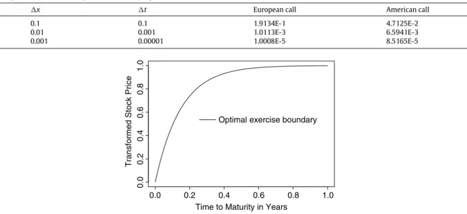
_. 5. Optimal exercise boundary

This section investigates the properties of optimal exercise boundary (i.e., free boundary) of American lookback options. we will show the existence and convergence of the approximate optimal exercise boundary in the BTM(2.20). We also achieve the terminal values

(

T

)

of the optimal exercise boundarys

(

t

)

of problem(3.2).

To prove the existence of approximate optimal exercise boundary in the BTM(2.20), it suffices to show the following results.

(11)

Lemma 5.1. Let1t be sufficiently small. For each n

<

N, there exists an integer jnsuch that



v

n j

=

1

−

u −j

_>

_In+1 j

,

j

≥

jn

v

n j

=

I n+1 j

≥

1

−

u −j

_,

_j

_<

_j n (5.1)

where I_jn+1is the simplified notation defined in(4.6). Furthermore, we have jn

≤

jn−1.

Proof. We use induction to prove this lemma. Ifj

≥

1, we have

ρ

I_jN

=

(

1

− ˆ

λ)

[

pu

v

_j+N₁

+

(

1

−

p

)

u−1

v

_j−N₁

] + ˆ

λ

+∞

−

l=−j+1 ul

v

N_j+lpl

+ ˆ

λ

−j

−

l=−∞ ul

v

₀Npl

=

(

1

− ˆ

λ)

[

pu

(

1

−

u−(j+1)

)

+

(

1

−

p

)

u−1

(

1

−

u−(j−1)

)

] + ˆ

λ

+∞

−

l=−j+1 ul

(

1

−

u−(j+l)

)

pl

=

(

1

− ˆ

λ)

[

pu

+

(

1

−

p

)

u−1

−

u−j

] + ˆ

λ

+∞

−

l=−j+1 ulpl

− ˆ

λ

u−j +∞

−

l=−j+1 pl

=

e(r−q)1t

− ˆ

λ(

1

+

k

)

+ ˆ

λ

+∞

−

l=−j+1 ulpl

−

u−j

+ ˆ

λ

u−j

− ˆ

λ

u−j +∞

−

l=−j+1 pl

=

e(r−q)1t

− ˆ

λ

−

l∈Z ulpl

+ ˆ

λ

+∞

−

l=−j+1 ulpl

−

u−j

+ ˆ

λ

u−j

−

l∈Z pl

− ˆ

λ

u−j +∞

−

l=−j+1 pl

+

O

(

1t 3 2

)

=

e(r−q)1t

+ ˆ

λ

−j−1

−

l=−∞

(

u−j

−

ul

)

pl

−

u −j

₊

_O

₍

₁_t32

),

where the fourth and fifth equalities follow from(4.4)and(4.5). Then

I_jN

−

(

1

−

u−j

)

=

e−r1t



e(r−q)1t

+

λ

1t −j−1

−

l=−∞

(

e−j1x

−

el1x

)

pl

−

e−j1x



−

1

+

e−j1x

+

O

(

1t32

)

=

(

1

−

r1t

)



1

+

(

r

−

q

)

1t

+

λ

1t −j−1

−

l=−∞

(

e−j1x

−

el1x

)

pl

−

e−j1x



−

1

+

e−j1x

+

O

(

1t32

)

=

(

re−j1x

−

q

)

1t

+

λ

1t −j−1

−

l=−∞

(

e−j1x

−

el1x

)

pl

+

O

(

1t 3 2

).

Noting that −j−1

−

l=−∞

(

e−j1x

−

el1x

)

pl

≥

−j−2

−

l=−∞

(

e−j1x

−

el1x

)

pl

≥

−(j+1)−1

−

l=−∞

(

e−(j+1)1x

−

el1x

)

pl

,

0

≤

−j−1

−

l=−∞

(

e−j1x

−

el1x

)

pl

≤

e−j1x

,

we can easily derive that, for1tsmall enough andj

≥

1

,

IN

j

−

(

1

−

u−j

)

is strictly monotonically decreasing with respect tojand whenjis sufficiently large, we must haveIN

j

−

(

1

−

u−j

) <

0. Forj

=

0, we can similarly derive

I₀N

−

(

1

−

u0

)

≥

I₁N

−

(

1

−

u1

).

So take m1

=

inf



j

≥

0

:

re−j1x

−

q

+

λ

−j−1

−

l=−∞

(

e−j1x

−

el1x

)

pl

≤

0



.

(5.2) IfIN m1

<

1

−

u −m1_{, let}_j N−1

=

m1; ifImN1

=

1

−

u −m1_{, let}_j

N−1

=

m1

+

1. Thus we have shown that there existsjN−1

=

m1or m1

+

1 such that(5.1)holds.

Suppose that(5.1)is true whenn

=

m

+

1. Whenj

<

jm+1, due toLemma 4.1(2), we have I_jm+1

≥

I_jm+2

≥

1

−

u−j

,

(12)

which implies thatjm

≥

jm+1ifjmexists. Whenj

≥

jm+1

+

1, we have

ρ

I_jm+1

=

(

1

− ˆ

λ)

[

pu

v

_j+m+₁1

+

(

1

−

p

)

u−1

v

_j−m+₁1

] + ˆ

λ

+∞

−

l=−j+1 ul

v

m+_j+l1pl

+ ˆ

λ

−j

−

l=−∞ ul

v

₀m+1pl

=

(

1

− ˆ

λ)

[

pu

(

1

−

u−(j+1)

)

+

(

1

−

p

)

u−1

(

1

−

u−(j−1)

)

]

+ ˆ

λ

+∞

−

l=jm+1−j ul

(

1

−

u−(j+l)

)

pl

+ ˆ

λ

jm+1−j−1

−

l=−j+1 ul

v

m+_j+l1pl

+ ˆ

λ

−j

−

l=−∞ ul

v

₀m+1pl

=

e(r−q)1t

− ˆ

λ

−

l∈Z ulpl

−

(

1

− ˆ

λ)

u−j

+ ˆ

λ

+∞

−

l=jm+1−j ul

(

1

−

u−(j+l)

)

pl

+ ˆ

λ

jm+1−j−1

−

l=−j+1 ul

v

_j+lm+1pl

+ ˆ

λ

−j

−

l=−∞ ul

v

m+₀ 1pl

+

O

(

1t 3 2

),

where the last equality follows from(4.4)and(4.5). Noting

−

l∈Z ulpl

−

u−j

=

−

l∈Z

(

ul

−

u−j

)

pl

=

−

l∈Z ul

(

1

−

u−(l+j)

)

pl

,

we have I_jm+1

−

(

1

−

u−j

)

=

e−q1t

−

e−r1tu−j

−

λ

1t

−

l∈Z ul

(

1

−

u−(l+j)

)

pl

+

λ

1t +∞

−

l=jm+1−j ul

(

1

−

u−(l+j)

)

pl

+

λ

1t jm−j−1

−

l=−j+1 ul

v

_j+lm+1pl

+

λ

1t −j

−

l=−∞ ul

v

₀m+1pl

−

1

+

u−j

+

O

(

1t 3 2

)

=

(

re−j1x

−

q

)

1t

+

λ

1t jn+1−j−1

−

l=−j+1 ul

[

v

_j+lm+1

−

(

1

−

u−(l+j)

)

]

pl

+

λ

1t −j

−

l=−∞ ul

[

v

m+₀ 1

−

(

1

−

u−(j+l)

)

]

pl

+

O

(

1t 3 2

).

It is easy to verify that jm+1−j−1

−

l=−j+1 ul

[

v

_j+lm+1

−

(

1

−

u−(l+j)

)

]

pl

+

−j

−

l=−∞ ul

[

v

m+₀ 1

−

(

1

−

u−(j+l)

)

]

pl

≥

jm+1−j−2

−

l=−j ul

[

v

_j+lm+1

−

(

1

−

u−(l+j)

)

]

pl

+

−j−1

−

l=−∞ ul

[

v

₀m+1

−

(

1

−

u−(j+l)

)

]

pl

≥

jm+1−(j+1)−1

−

l=−(j+1)+1 ul

[

v

m+_(j+₁1₎_+l

−

(

1

−

u−(l+j+1)

)

]

pl

+

−(j+1)

−

l=−∞ ul

[

v

m+₀ 1

−

(

1

−

u−(l+j+1)

)

]

pl

,

where the last inequality follows fromLemma 4.1(4).

Then we conclude thatI_jm+1

−

(

1

−

u−j

₎

_{is strictly monotonically decreasing towards}_j_when_j

_≥

_j

m+1

+

1. Because

v

m+1

jm+1−1

≥

1

−

u

−(jm+1−1)_{, we can similarly derive that}

I_jm+1

m+1

−

(

1

−

u

−jm+1

)

_≥

_Im+1

jm+1+1

−

(

1

−

u

−(jm+1+1)

).

So this monotonicity holds true forj

≥

jm+1. FromLemma 4.1(3), we can easily get that

0

≤

λ

−j

−

l=−∞ ul

[

v

m₀+1

−

(

1

−

u−(j+l)

)

]

pl

≤

λ

−j

−

l=−∞ u−jpl

≤

λ

e−j1x

,

0

≤

λ

jm+1−j−1

−

l=−j+1 ul

[

v

_j+lm+1

−

(

1

−

u−(j+l)

)

]

pl

≤

λ

jm+1−j−1

−

l=−j+1 ujm+1−j_p l

≤

λ

ejm+1−j1x

.