econstor
www.econstor.eu
Der Open-Access-Publikationsserver der ZBW – Leibniz-Informationszentrum Wirtschaft
The Open Access Publication Server of the ZBW – Leibniz Information Centre for Economics
Nutzungsbedingungen:
Die ZBW räumt Ihnen als Nutzerin/Nutzer das unentgeltliche, räumlich unbeschränkte und zeitlich auf die Dauer des Schutzrechts beschränkte einfache Recht ein, das ausgewählte Werk im Rahmen der unter
→ http://www.econstor.eu/dspace/Nutzungsbedingungen nachzulesenden vollständigen Nutzungsbedingungen zu vervielfältigen, mit denen die Nutzerin/der Nutzer sich durch die erste Nutzung einverstanden erklärt.
Terms of use:
The ZBW grants you, the user, the non-exclusive right to use the selected work free of charge, territorially unrestricted and within the time limit of the term of the property rights according to the terms specified at
→ http://www.econstor.eu/dspace/Nutzungsbedingungen By the first use of the selected work the user agrees and declares to comply with these terms of use.
zbw
Dette, Holger; Birke, Melanie
Working Paper
Estimating a convex function in
nonparametric regression
Technical Report / Universität Dortmund, SFB 475 Komplexitätsreduktion in Multivariaten Datenstrukturen, No. 2005,21
Provided in cooperation with: Technische Universität Dortmund
Suggested citation: Dette, Holger; Birke, Melanie (2005) : Estimating a convex function in nonparametric regression, Technical Report / Universität Dortmund, SFB 475 Komplexitätsreduktion in Multivariaten Datenstrukturen, No. 2005,21, http:// hdl.handle.net/10419/22612
Estimating a convex function in nonparametric regression
Melanie Birke
Ruhr-Universit¨at Bochum
Fakult¨at f¨
ur Mathematik
44780 Bochum, Germany
e-mail: [email protected]Holger Dette
Ruhr-Universit¨at Bochum
Fakult¨at f¨
ur Mathematik
44780 Bochum, Germany
e-mail: [email protected] FAX: +49 2 34 32 14 559July 1, 2005
AbstractA new nonparametric estimate of a convex regression function is proposed and its stochastic properties are studied. The method starts with an unconstrained estimate of the derivative of the regression function, which is firstly isotonized and then integrated. We prove asymptotic normality of the new estimate and show that it is first order asymptotically equivalent to the initial unconstrained estimate if the regression function is in fact convex. If convexity is not present the method estimates a convex function whose derivative has the sameLp-norm as the derivative of the (non-convex) underlying regression function. The finite sample properties of the new estimate are investigated by means of a simulation study and the application of the new method is demonstrated in two data examples.
AMS Subject classification: 62G05, 62G07
Keywords and Phrases: nonparametric regression, order restricted inference, convexity, Nadaraya-Watson estimate, nondecreasing rearrangement
1
Introduction
The estimation of functions under shape restrictions is an important problem in the analysis of the relationship among variables. In many settings experimenters are in the position of having strong presumptions that these relationships satisfy certain qualitative restrictions such as monotonicity, convexity or concavity. Typical examples appear in economics (indirect utility, production or cost functions), medicine (dose response experiments) or biology (growth curves). Much effort has been spent to the problem of estimating a monotone regression function using the least squares approach [see e.g. Brunk (1955), Mukerjee (1988) among others and Barlow, Bartholomew, Bremner and
Brunk (1972) or Robertsen, Wright and Dykstra (1988) for a summary of this work]. In the case of concave (convex) regression a concave (convex) least squares estimate was first proposed by Hildreth (1954) and its consistency was proved by Hanson and Pledger (1976). Some algorithms for the calculation of the concave (convex) least squares estimate can be found in Wu (1982) and Fraser and Massam (1989). Mammen (1991) derived the rate of convergence of a least squares estimator of a convex or concave regression function and its derivative at a fixed point, while recently Groeneboom, Jongblood and Wellner (2001) proved consistency and derived the asymptotic distribution of the estimator at a fixed point of positive curvature.
In the present paper we propose an alternative estimate of a convex or concave regression function, which is not based on the least squares technique and particularly attractive to users of conventional smoothing methods. We will restrict ourselves to the case of convexity, but the case of concavity will be obvious from our discussion (see also the second example in Section 5). On the one hand our work is motivated by the fact that the commonly used least squares technique and also other projection based techniques produce a rather unsmooth convex estimate, even if the underlying regression function “is known” to be smooth. On the other hand we are interested in a simple and computationally efficient convex estimate, because convex estimates of the regression function are usually calculated by successive projections [see e.g. Dykstra (1983) or Han (1988)] and these iterative procedures can be very slow in some cases.
The new estimate is obtained in several steps. We first estimate the derivative of the regression function, which is isotonized in a second step to obtain a strictly isotone and smooth estimate of the derivative of the regression function. In a final step this estimate is integrated to obtain a strictly convex regression estimate, which is (at least) two times continuously differentiable. We prove consistency and asymptotic normality of the new estimate with the common rates of convergence in nonparametric regression. In particular first order asymptotic equivalence of the new convex estimator to the unconstrained estimate is established, if the underlying regression is in fact convex. Otherwise it is shown that the procedure proposed in this paper produces a convex curve, whose
derivative has for any p > 0 the same Lp-norm as the derivative of the given regression function.
Because of its simplicity the new method is particularly appealing to users of conventional kernel methods if some prior knowledge regarding the smoothness of the regression function is available. Our approach is carefully explained in Section 2, where we also study its main properties from an asymptotic point of view. Some further properties of the new estimate are discussed in Section 3, while the finite sample performance of the new method is investigated in Section 4 by means of a simulation study. In Section 5 two data examples are investigated and the application of the new procedure is illustrated. Finally, all proofs and technical details are deferred to an Appendix. It is also remarkable that the procedure proposed in this paper is universally applicable to other problems of convex or concave estimation (for example convex density or hazard rate estimation or the convex estimation of a parametric curve). Whenever an unconstrained estimate of a convex (or concave) curve in a particular estimation problem is available, and the method is applied to this preliminary estimator, the resulting curve estimator is convex (or concave) and first order asymptotic equivalent to the unconstrained preliminary estimate. However, for the sake of brevity and definiteness this paper is restricted to the problem of estimating a nonparametric convex regression curve.
2
Convex estimation
Consider the common nonparametric regression model
Yi =m(Xi) +σ(Xi)εi i= 1, . . . , n,
(2.1)
where X1, . . . , Xn are i.i.d. random variables with density f : [0,1] →R bounded away from zero
and ε1, . . . , εn are i.i.d. independent of X1, . . . , Xn with mean 0, variance 1 and existing fourth
moment. We assume that the variance functionσ2 : [0,1]→R+ is continuous and that the density
and regression function are three times continuously differentiable. We note that m is strictly
convex if and only if its derivative m0
is strictly increasing. Therefore we first construct a strictly isotone estimate of the derivative of the regression function which will be integrated in a second step. For this purpose any unconstrained nonparametric estimate (kernel type, local polynomial, series or spline estimator) of the regression function could be used. For the sake of definiteness we consider the Nadaraya-Watson estimate and some remarks regarding a local linear estimate can
be found in Remark 2.3. To be precise let Kr denote a kernel of order three [see Gasser, M¨uller
and Mammitzsch (1985)] with compact support, say [−1,1], which is three times continuously
differentiable with Lipschitz continuous third derivative and define the kernel estimator of the
derivative of order p ∈ N of the regression function as ˆm(p)(x) = ∂p
∂xpmˆ(x) where ˆm denotes the
Nadaraya-Watson estimate given by ˆ m(x) = Pn i=1Kr(x −Xi hr )Yi Pn i=1Kr(x−hrXi) (2.2)
[see Nadaraya (1964) or Watson (1964)]. Herehr denotes a bandwidth converging to 0 with
increas-ing sample size and the kernelKr has been appropriately modified in order to address for boundary
effects [see e.g. M¨uller (1985)]. Following Dette, Neumeyer and Pilz (2005) we consider a further
kernel, say Kd, with compact support which is two times continuously differentiable with second
derivative bounded away from zero and a bandwidth hd and define
ˆ ψhd(t) = 1 hd Z 1 0 Z t −∞ Kd ˆ m0 (v)−u hd dudv (2.3)
as an estimate of the inverse function ofm0
,say (m0
)−1 at the pointt. Note that the function in (2.3)
is strictly increasing if hd is sufficiently small and consequently its inverse is a strictly isotone and
smooth estimate of the derivative of the regression function. Finally, the strictly convex estimate
of the regression function m is defined by
ˆ mC(x, u0) = ˆm(u0) + Z x u0 ˆ ψ−1 hd(z)dz, (2.4) where ˆψ−1
hd denotes the inverse of the function ˆψhd and (at the moment) u0 ∈(0,1) is an arbitrary
point. The choice of u0 will be carefully discussed in Section 3. Note that the estimate ˆmC is
obviously strictly convex because its derivative ˆψ−1
hd is strictly increasing by our construction.
Before we study the main asymptotic properties of our method we will present an alternative inter-pretation of our approach. The main idea is similar to the concept of nondecreasing rearrangements
[see Ryff (1965, 1970) or Bennett and Sharpely (1988)]. To be precise let g be a continous function
with domain [0,1] and range R(g) ⊆ R. We define an operator ψ on C([0,1]), which maps the
function g to the function
ψ(g) : ( R(g) → [0,1] t → ψ(g)(t) =R [0,1]I{g(x)≤t}dx . (2.5)
Obviously, we have for a strictly isotone function g
ψ(g) = g−1 onR(g),
(2.6)
On the other hand, the function ψ(g) is always isotone independently if the function g possesses
this property. In the following we denote byψ−1(g) the inverse of the functionψ(g), then it follows
by similar arguments as given in Birke and Dette (2005) that for any continuous function g the
identity Z [0,1]| g(x)|pdx= Z [0,1]| ψ−1(g)(x)|pdx (2.7)
holds for all p ∈(0,∞]. In other words: the function ψ−1(g) is increasing on the domain of g, has
the sameLp-norm as the function g and coincides with g if this function is itself strictly increasing.
In this sense the function ψ−1
(g) can be considered as a monotone approximation of the function
g. Note that the function ψ−1(g) is not necessarily differentiable. However, smoothing can easily
be accomplished by replacing ψ in (2.5) by the operatorψhd(g) :R→R defined by
ψhd(g)(t) = 1 hd Z [0,1] Z t −∞ Kd g(x)−u hd dudx, (2.8)
where hd denotes a further bandwidth, which converges to 0 sufficiently fast. The function ψhd(g)
is obviously differentiable and a standard calculation shows ψhd(g) = ψ(g) +o(1). In the present
context we apply this concept to the function m0
and denote by ψ−1
hd(g) the inverse of the function
ψhd(g). Note that ψhd( ˆm
0
) = ˆψhd corresponds to the estimate (2.3) and that heuristically (if m
0 is strictly increasing) ˆ ψhd−(m 0 )−1 = ψ hd( ˆm 0 )−ψ(m0 )≈ψhd( ˆm 0 )−ψhd(m 0 ) (2.9) ≈ ∂λ∂ ψhd(m 0 +λ( ˆm0 −m0 ))|λ=0 ≈ − mˆ0−m0 m00 ◦(m0 )−1
Applying this heuristic argument a second time [basically replacing ˆψhd by ˆψ
−1 hd and m 0 by (m0 )−1] yields ˆ ψ−1 hd −m 0 ≈ −ψˆhd−(m 0 )−1 ((m0)−1)0 ◦m0 ≈mˆ0 −m0 ,
where we used the representation (2.9) for the last approximation. Finally, we obtain from (2.10) for the convex estimate in (2.4)
ˆ mC(x, u0)−m(x) = ˆm(u0)−m(u0) + Z x u0 ˆ ψh−d1(z)−m0(z)dz ≈ mˆ(x)−m(x).
Therefore, if the regression function m is strictly convex, we expect that the new convex estimate ˆ
mC exhibits the same asymptotic behaviour as the unconstrained Nadaraya-Watson estimate of the
regression function.
A detailed proof of such a statement is substantially more complicated and presented in the Ap-pendix. For this purpose we require the following basic assumptions regarding the smoothing
parameters in the estimates. The bandwidths hd and hr in the estimates (2.2) and (2.3) have to
satisfy hd, hr → 0 (2.11.a) nhd, nhr → ∞ (2.11.b) hd/h3r/2 → 0 (2.11.c) nh7r = O(1) (2.11.d) (logh−1 r )3/2/nh4rh2d = o(1) (2.11.e)
if the sample size n converges to infinity. Our main results make the heuristic arguments of the
previous paragraph precise.
Theorem 2.1. Assume that the assumptions stated at the beginning of Section 2 and in (2.11.a)-(2.11.e) are satisfied. If the regression function m in (2.1) is strictly convex, then we have for any
x∈(0,1)with m00 (x)>0 and any u0 ∈(0,1) ˆ mC(x, u0)−m(x) = ˆm(x)−m(x) +op 1 √ nhr (2.12)
Corollary 2.2. If the assumptions of Theorem 2.1 are satisfied, then p
nhr( ˆmC(x, u0)−m(x)−bn(x))
D
→ N(0, γ(x)) (2.13)
for any x, u0 ∈(0,1), where the asymptotic bias and variance are given by
bn(x) = h3rκ3(Kr) (mf)(3)−mf(3) f (x) +o h 3 r , γ(x) = Z 1 −1 Kr2(y)dyσ 2 f (x), respectively and κ3(Kr) = 1/3! R1 −1u 3K r(u)du.
Remark 2.3. Note that Theorem 2.1 and Corollary 2.2 show that the convex estimate ˆmC(x, u0)
is first order asymptotic equivalent to the preliminary unconstrained Nadaraya-Watson estimate ˆm
[see e.g. H¨ardle (1991)].
Moreover, a careful inspection of the proofs in the appendix shows that similar results can be
derived, if alternative smoothing procedures are used as preliminary estimate. For example if ˆm0
is the derivative of a local polynomial estimate [see Fan and Gijbels (1996)] the asymptotic statement (2.13) is still true, where the bias has to be replaced by
˜bn(x) =h3
3
Further discussion
In this section we briefly discuss the choice of the initial point u0 ∈ (0,1) which is crucial for
the performance of the proposed procedure. For the sake of a transparent presentation we begin with the deterministic case, where the estimators in (2.4) have been replaced by their deterministic counterparts. The transfer to the estimates considered in Section 2 will be obvious from our discussion and is briefly mentioned at the end of this section.
Recall the definition of the function ψ and ψhd in (2.5) and (2.8), respectively, and note that any
function of the form
mC(x, u0) = m(u0) + Z x u0 ψ−1 hd(m 0 )(t)dt (3.1)
is strictly convex. Moreover, if m0
is strictly increasing (in other words m is strictly convex) and
hd →0 we have ψh−d1(m0)→m0 and as a consequence
mC(x, u0)−→
hd→0
m(x) for all x, u0 ∈(0,1).
(3.2)
In this case the choice of the point u0 is irrelevant, provided that hd is sufficiently small. On
the other hand, it is also important to discuss the impact of the choice of u0 in the case, where
m is not convex, because in applications the preliminary estimate ˆm will rarely be convex (or
its derivative ˆm0
isotone). If m is not convex each function mC(·, u0) with u0 ∈ (0,1) defines a
“convex rearrangement” of the function m(·) whose derivative has approximately (if hd → 0) the
same Lp-norm as the initial unconstrained function m. We will discuss further properties of this
rearrangement in the following.
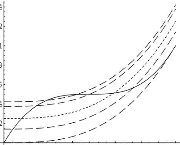
Example 3.1. In order to fix ideas we have illustrated the situation for the function
m(x) = 1 2 + 1 2(2x−1) 3 x∈[0,1] (3.3)
in Figure 1, which is obviously neither convex nor concave. In this case we calculate the limit of
(3.1) as hd →0, that is ¯ mC(x, u0) =m(u0) + Z x u0 ψ−1(m0 )(t)dt. (3.4) We have ψ(m0 )(t) = r t 3; t ∈[0,3], which gives ψ−1(m0 )(t) = 3t2 and ¯ mC(x, u0) = m(u0) + Z x u0 ψ−1(m0 )(t)dt (3.5) = 1 2+ 1 2(2u0−1) 3 −u30+x3
as convex rearrangement of the function m. In Figure 1 we display several of these functions and
0.2 0.4 0.6 0.8 1 0.2 0.4 0.6 0.8 1 1.2 1.4
Figure 1: The function m defined in (3.3) (solid line) and several convex rearrangements m¯C(·, u0)
defined by (3.4) with u0 = 0,0.25,0.5 and 0.75 (dashed lines). The dotted line corresponds to the
best L2-approximation of the function m by the class {m¯
C(x, u0)|u0 ∈[0,1]} defined in (3.5).
m(x) are given by 3x2 and 3(2x−1)2, respectively, and that both functions have for all p >0 the
same Lp-norm on the interval [0,1].
If m is not strictly convex, an appropriate convex approximation of the function m by elements of
the form (3.1) is now determined by minimizing the L2-norm
Φ(u0) =
Z 1
0
(m(x)−mC(x, u0))2dx
(3.6)
over the interval (0,1).Our main result of this section characterizes the solution of this
approxima-tion problem.
Theorem 3.2. Let Ψhd denote any function with (Ψhd)
0 =ψ−1 hd(m 0 ). A point u∗ 0 ∈(0,1)minimizes
the function Φ defined in (3.6) if and only if
m(u∗ 0)−Ψhd(u ∗ 0) = Z 1 0 (m(u)−Ψhd(u))du. (3.7)
Moreover, we have for any u∗
0 minimizing (3.6) mC(x, u∗0) = Z 1 0 mC(x, u)du. (3.8)
In other words: the function on the right hand side of (3.8) is of the form (3.1) and minimizes the
Example 3.3. In the situation considered in Example 3.1 we have Ψhd → Ψ if hd → 0, where Ψ0 =ψ−1(m0 ), that is m(u)−Ψ(u) = 1 2 + 1 2(2u−1) 3 −u3, Z 1 0 (m(u)−Ψ(u))du = 1 4.
The solutions of the analogue of equation (3.7) in the interval (0,1) are given by
u∗0,1 ≈0.103741; u∗0,2 ≈0.638824,
and both points correspond to the best L2-approximation of the function (3.3) by elements of the
form (3.5); i.e. ¯ mC(x, u∗0,j) = Z 1 0 ¯ mC(x, u)du= 1 4+x 3.
The application of Theorem 3.2 for the construction of a convex estimator of the form (2.4) with
minimal L2-distance to the initial unconstrained estimate ˆm is now straightforward. Note that it
is not necessary to calculate the solution of the sample analogue of (3.7). The representation (3.8) can be applied directly and
ˆ mC(x) := Z 1 0 ˆ mC(x, u0)du0 (3.9)
yields the convex estimate, which has minimalL2-distance to the unconstrained regression estimate
ˆ
m in the class
{mˆC(x, u0)|u0 ∈(0,1)}
defined by (2.4). We finally remark that the computational effort for the numerical evaluation of the integral in (3.9) can be decreased observing the relation
ˆ
mC(x, u0) = ˆm(x) + ˆm(u0)−mˆC(u0, x),
which is obvious from the representation (2.4).
4
Finite sample properties
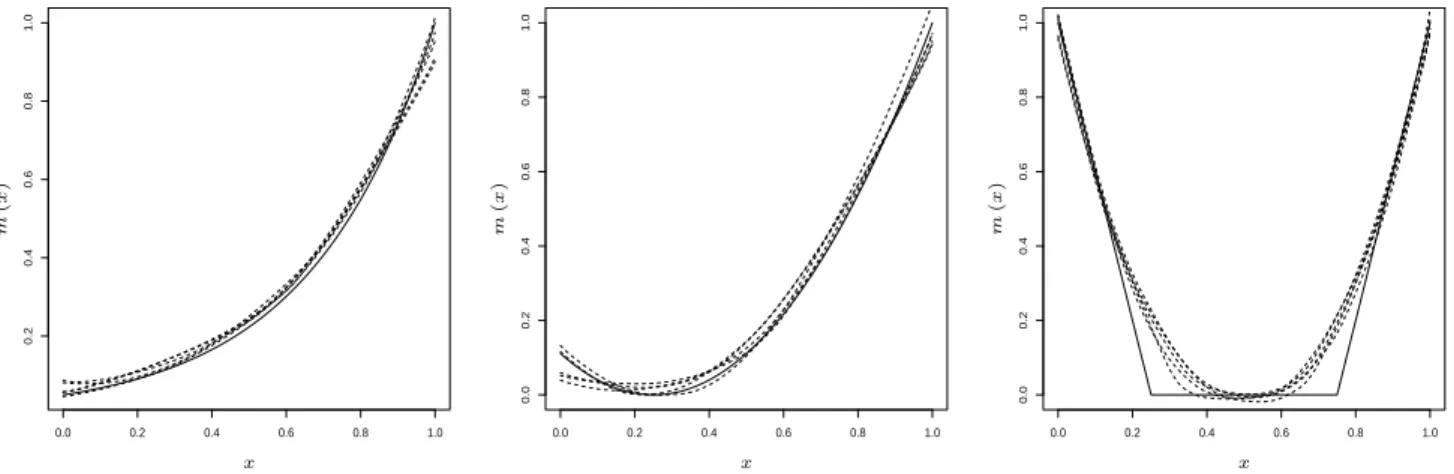
In this section we briefly illustrate the finite sample properties of the convex estimate of the regres-sion function by means of a simulation study. For this purpose we consider three examples
m(x) = e3(x−1), (4.1) m(x) = 16 9 (x− 1 4) 2, (4.2) m(x) = −4x+ 1 if 0≤x≤ 14 0 if 1 4 ≤x≤ 3 4 4x−3 if 34 ≤x≤1. (4.3)
0.0 0.2 0.4 0.6 0.8 1.0 0.2 0.4 0.6 0.8 1.0 PSfrag replacements x m ( x ) m(x) 0.0 0.2 0.4 0.6 0.8 1.0 0.0 0.2 0.4 0.6 0.8 1.0 PSfrag replacements x m ( x ) m(x) 0.0 0.2 0.4 0.6 0.8 1.0 0.0 0.2 0.4 0.6 0.8 1.0 PSfrag replacements x m(x) m ( x )
Figure 2: The regression functions (4.1) (left part), (4.2) (middle part) and (4.3) (right part) and
five convex estimates from different simulation runs. The sample size is n = 100 and the standard
deviation is σ= 0.1.
Note that all functions are convex but in contrast to the functions in (4.1) and (4.2) the function in (4.3) does not satisfy the assumptions required for the asymptotic theory in Section 2. The errors in the regression model (2.1) are assumed to be normal and homoscedastic with standard deviation
σ = 0.1, while a uniform design was simulated for the explanatory variables. We used a sample of
n = 100 observations to estimate the regression function. In the following ˆσ2 denotes the estimator
of the integrated variance proposed by Rice (1984). For the preliminary (unconstrained) estimate
of m0
the derivative of the local linear estimate was used in order to address for boundary effects.
The bandwidth hr in this estimate was chosen by
hr =
σˆ2
n
1/7 (4.4)
which is proportional to the asymptotical optimal bandwidth for a three times continuously
dif-ferentiable regression and density function while the bandwidth hd for the density step is given
by
hd =h8r/5.
(4.5)
The kernelsKd andKr are both chosen as Epanechnikov kernel. For the selection of the pointu0 we
used the best L2-approximation proposed in Section 3, where the integral in (3.9) is approximated
by a Riemann sum. In Figure 2 we display for each regression function five typical estimates obtained from different simulation runs. We observe a reasonable performance of the estimates for the regression functions (4.1) and (4.2). In example (4.3) the estimate does not precisely reproduce the true function at points where the regression function is not differentiable, but in the regions where the derivative is two times differentiable the estimates are again very reliable.
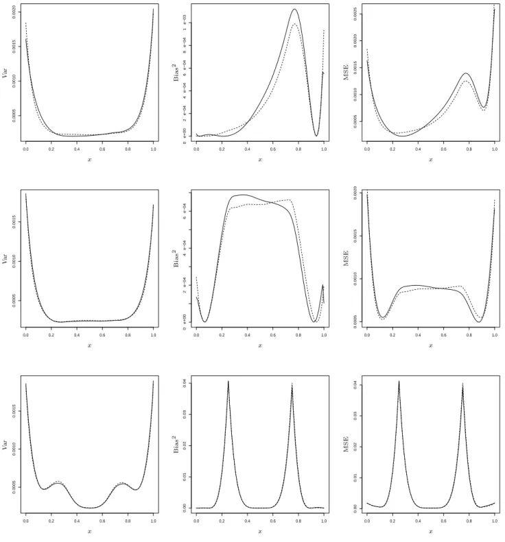
In the second part of this simulation study we investigate the mean squared error, bias and variance of the convex estimator proposed in this paper. For this we consider again the three regression functions in (4.1) - (4.3) and calculate by 2000 simulation runs the curves for the mean squared
0.0 0.2 0.4 0.6 0.8 1.0 0.0005 0.0010 0.0015 0.0020 PSfrag replacements x V ar MSE Bias2 MSE Bias2 0.0 0.2 0.4 0.6 0.8 1.0 0 e+00 2 e−04 4 e−04 6 e−04 8 e−04 1 e−03 PSfrag replacements x Var MSE Bias 2 MSE Bias2 0.0 0.2 0.4 0.6 0.8 1.0 0.0005 0.0010 0.0015 0.0020 0.0025 PSfrag replacements x Var MSE Bias2 MSE Bias2 0.0 0.2 0.4 0.6 0.8 1.0 0.0005 0.0010 0.0015 PSfrag replacements x V ar MSE Bias2 MSE Bias2 0.0 0.2 0.4 0.6 0.8 1.0 0 e+00 2 e−04 4 e−04 6 e−04 PSfrag replacements x Var MSE Bias 2 MSE Bias2 0.0 0.2 0.4 0.6 0.8 1.0 0.0005 0.0010 0.0015 0.0020 PSfrag replacements x Var MSE Bias2 MSE Bias2 0.0 0.2 0.4 0.6 0.8 1.0 0.0005 0.0010 0.0015 PSfrag replacements x V ar MSE Bias2 MSE Bias2 0.0 0.2 0.4 0.6 0.8 1.0 0.00 0.01 0.02 0.03 0.04 PSfrag replacements x Var MSE Bias2 MSE Bias 2 0.0 0.2 0.4 0.6 0.8 1.0 0.00 0.01 0.02 0.03 0.04 PSfrag replacements x Var MSE Bias2 MSE Bias2
Figure 3: Simulated variance, squared bias and mean squared error of the convex estimator mˆC
(solid line) and the local linear estimate mˆ (dashed line). The sample size is n= 100, the standard deviation is σ = 0.1, while the regression functions are given by (4.1) (upper panel), (4.2) (middle panel) and (4.3) (lower panel), respectively.
error, squared bias and variance. The results are depicted in Figure 3 for all three cases under consideration. In this figure the local linear (unconstrained) estimate is represented by the dashed
line, while the new convex estimate ˆmC is depicted by the solid line. As predicted by the asymptotic
theory only small differences between the unconstrained and convex estimates are observed. In the
situation of example (4.1) we see that the squared bias of the local linear estimate ˆm is smaller if
x∈[0.4,0.9] while it is larger ifx∈[0.1,0.4]. Both estimates show a similar behaviour with respect
to the variance criterion, where there are slight advantages for the convex estimate in the interior of the design space. The mean squared error is dominated by the bias and smaller for the local
linear estimate in most parts of the interval [0,1] [see the first line in Figure 3].
For the regression function (4.2) we observe from the middle line of Figure 3 that the local linear
estimate yields a smaller (squared) bias than the convex estimate ˆmC ifx <0.6, while the converse
is true if x∈[0.6,0.9]. The variance of the convex estimate is slightly smaller than the variance of
the local linear estimate. Because the variance of both estimates is very similar, a comparison of
the mean squared error curves shows some advantages for the constrained estimate if x >0.6 and
a smaller mean squared error of the local linear estimate if x <0.6. Again the bias dominates the
mean squared error. For the regression function (4.3) the situation is slightly different. Here both estimates have a similar variance, but there are some (small) advantages for the convex estimate in a neighbourhood of points, where the regression function is not differentiable [see the left lower panel in Figure 3]. The squared bias curves of both estimates are very similar. Again the squared bias of the local linear estimate is larger at points where the derivative of the regression function is discontinuous. In these regions the mean squared error is dominated by the squared bias, which is reflected in the right panel of the third line of Figure 3.
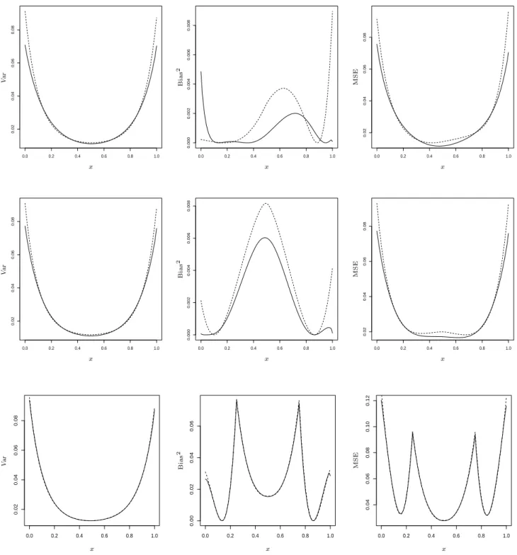
Note that in these examples the bias dominates the variance. A partial explanation of this obser-vation stems from the fact that the variance of the errors of the simulated obserobser-vations is rather
small, namely σ2 = 0.01. In order to compare the unconstrained and convex estimate in the case
of a larger variance we present in Figure 4 the simulated variance, squared bias and mean squared
error curves for the functions (4.1) - (4.3), where the simulated observations have variance σ2 = 1.
In example (4.3) the squared bias and variance are of the same size and there are no substantial visual differences compared to the case considered in Figure 3 [see the last lines in Figure 3 and 4]. However, in example (4.1) and (4.2) the situation is different and the variance dominates the squared bias. In these two examples the variance curves of both estimates show a similar behaviour with small advantages for the convex estimate [see the left panel in the first and second line of Figure 4], while the squared bias of the local linear estimate is larger than that of the constrained estimate [see the middle panels]. As a consequence the mean squared error of the new convex estimate is usually smaller than the mean squared error of the local linear estimate [see the right panel in the first and second line of Figure 4].
0.0 0.2 0.4 0.6 0.8 1.0 0.02 0.04 0.06 0.08 PSfrag replacements x Var MSE Bias2 V ar MSE Bias2 MSE Bias2 0.0 0.2 0.4 0.6 0.8 1.0 0.000 0.002 0.004 0.006 0.008 PSfrag replacements x Var MSE Bias2 Var MSE Bias 2 MSE Bias2 0.0 0.2 0.4 0.6 0.8 1.0 0.02 0.04 0.06 0.08 PSfrag replacements x Var MSE Bias2 Var MSE Bias2 MSE Bias2 0.0 0.2 0.4 0.6 0.8 1.0 0.02 0.04 0.06 0.08 PSfrag replacements x Var MSE Bias2 V ar MSE Bias2 MSE Bias2 0.0 0.2 0.4 0.6 0.8 1.0 0.000 0.002 0.004 0.006 0.008 PSfrag replacements x Var MSE Bias2 Var MSE Bias 2 MSE Bias2 0.0 0.2 0.4 0.6 0.8 1.0 0.02 0.04 0.06 0.08 PSfrag replacements x Var MSE Bias2 Var MSE Bias2 MSE Bias2 0.0 0.2 0.4 0.6 0.8 1.0 0.02 0.04 0.06 0.08 PSfrag replacements x V ar MSE Bias2 Var MSE Bias2 MSE Bias2 0.0 0.2 0.4 0.6 0.8 1.0 0.00 0.02 0.04 0.06 PSfrag replacements x Var MSE Bias2 Var MSE Bias2 MSE Bias 2 0.0 0.2 0.4 0.6 0.8 1.0 0.04 0.06 0.08 0.10 0.12 PSfrag replacements x Var MSE Bias2 Var MSE Bias2 MSE Bias2
Figure 4: Simulated variance, squared bias and mean squared error of the convex estimator mˆC
(solid line) and the local linear estimate mˆ (dashed line). The sample size is n= 100, the standard deviation is σ = 1, while the regression functions are given by (4.1) (upper panel), (4.2) (middle panel) and (4.3) (lower panel), respectively.
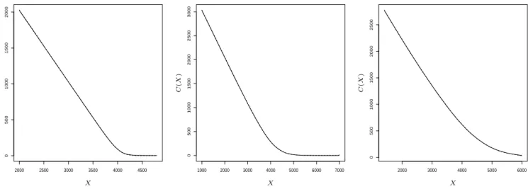
2000 2500 3000 3500 4000 4500 0 500 1000 1500 2000 PSfrag replacements C ( X ) X 1000 2000 3000 4000 5000 6000 7000 0 500 1000 1500 2000 2500 3000 PSfrag replacements C ( X ) X 2000 3000 4000 5000 6000 0 500 1000 1500 2000 2500 PSfrag replacements C ( X ) X
Figure 5: The local linear estimate (dotted line) and new convex estimate (solid line) of the call
pricing function of three DAX options considered as a function of the strike price. Left panel: February 9, 2004, expiration time 494 days; middle panel: January 2, 2004, expiration time 14 days; right panel: January 2, 2004; expiration time 168 days.
5
Examples
5.1
Estimation of a convex option pricing function
The call pricing function of a European option, say C,at time t usually depends on the underlying
asset price at date t, say St, the strike priceX,the time to expiration τ, the deterministic risk free
interest ratert,τ and the correspondend dividend yieldδt,τ of the asset. More precisely, this function
is given by
C(St, X, τ, rt,τ, δt,τ) = e−rt,τ
Z ∞
0
max{ST −X,0}p∗(ST |St, τ, rt,τ, δt,τ)dST,
where T =τ +t is the expiration date and p∗
denotes the state-price density, which is also called risk neutral density [see e.g. Black and Scholes (1973), or Cox, Ingersoll and Ross (1985)]. By
taking derivatives ofC with respect to X it was pointed out by A¨ıt-Sahalia and Duarte (2003) that
the function C must be decreasing and convex in X in order to rule out arbitrage opportunities.
In particular, any local non-convexity of the call pricing function implies negative state prices, violating the no-arbitrage principle.
We will now illustrate a possible application of the proposed procedure and construct a convex
estimate of the function C considered as a function of the strike price X. For this we analyze data
from a DAX-option, which was kindly provided by K. Pilz (Sal. Oppenheim Bank). The data shows for a particular day the strike price of the option, expiration time, volatility, call price and closing
price of the DAX. We construct a convex estimate of the call pricing function as a function ofX. As
preliminary estimate ˆm0
we use the derivative of a local linear estimator with bandwidthhr chosen
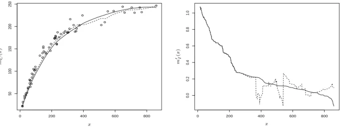
0 200 400 600 800 50 100 150 200 250 PSfrag replacements m C ( x ) x m0 I(x) x 0 200 400 600 800 0.0 0.2 0.4 0.6 0.8 1.0 PSfrag replacements mC(x) x m 0(I x ) x
Figure 6: Left panel: The local linear estimate mˆ (dotted line) and convex estimate mˆC (solid line)
of the dry weight (in milligrams) of the eye lense as a function of the age (in days) estimated from71 free-living wild rabbits. Right panel: the derivative mˆ0
of the local linear estimator and its antitone estimate ψ˜−1
hd defined by (5.1).
crucial. In Figure 5 we show the local linear and the new convex estimate of the call pricing function of a DAX option as a function of the strike price for 3 representative cases. The left part of Figure 5 corresponds to the price at February 9, 2004, where the expiration time is 494 days. Similarly, the middle and right panel of Figure 5 correspond to call option prices at January 2, 2004, where expiration time is 14 and 168 days, respectively. We observe that in all cases a similar picture. The
unconstrained estimate ˆm of the pricing function is convex and also decreasing as a function of the
strike price X. For this reason the convex estimate ˆmC essentially coincides with the local linear
estimate, which is definitely a desirable property of the new procedure. If the resulting convex
estimate ˆmC would not be decreasing it could be easily monotonized by the method described in
Dette, Neumeyer and Pilz (2005).
5.2
Rabbits data
In the previous example the local linear estimate was already convex and the new convex estimate basically reproduced the unconstrained estimate. We now consider a situation, where the local linear estimate does not satisfy the constraints of convexity or concavity. For this we use an example considered by Dudzinsky and Mykytowycz (1961), who analyzed the relation between age and eye lens weight for rabbits in Australia. In this study, the dry weight of the eye lens was measured (in milligrams) for 71 free-living wild rabbits of known age (measured in days). A detailed description of the experiment and the data can be found in http://www.statsci.org/data/oz/rabbit.html. The data was analyzed by Ratkowski (1983) using the nonlinear growth model
which is obviously concave with respect to the variablex. In the left panel of Figure 6 we display a local linear estimate and its “concave” rearrangement. A concave estimate is obtained by replacing the statistic ˆψ−1 hd in (2.4) by ˜ψ −1 hd, where ˜ ψhd(t) = 1 hd Z 1 0 Z ∞ t Kd ˆ m0 (v)−u hd dudv (5.1) (note that ˜ψ−1 hd is an antitone estimate of m 0
). The bandwidth for the unconstrained estimate is
again chosen by least square cross-validation while the bandwidthhd in the monotonizing procedure
is given by hd = h8r/5. We observe that the local linear estimate of the regression function is not
concave if the age of the rabbits is larger than 400 days. Therefore a monotonization of the derivative
is performed. The derivative of the local linear estimate and its antitone rearrangement ˜ψhd are
depicted in the right panel of Figure 6. The new method yields a concave estimate, which fits the data adequately and preserves the features of the unconstrained local linear estimate in regions where this is already concave.
6
Appendix: Proofs
Note that the estimate ˆψ−1
hd in the integral of (2.4) is obtained as the inverse of the estimate ˆψhd
defined in (2.3). It was shown in Dette, Neumeyer and Pilz (2005) that the operator, which maps a function onto its quantile (at a certain point) is two times Gat´eaux differentiable. In order to make the present paper self-contained we recall this result at the beginning of the proof.
Consider a fixed point t ∈ R, and let M denote the set of all functions H ∈ C2[0,1] with positive
derivative on the interval [0,1], which contain t in the interior of their image, i.e. t ∈ intH([0,1]).
Consider the functional
φ: (
M → [0,1]
H → H−1
(t)
and define for H1, H2 ∈ Mthe function
Q: (
[0,1] → R
λ → φ(H1+λ(H2−H1)).
(6.1)
Note that in the case of existence Q0
(0) is the Gat´eaux derivative of the functional φ at H1 in the
direction ofH2−H1.The following result shows that this derivative exists and also gives the second
derivative.
Lemma A.1. The mapping Q: [0,1]→R defined by (6.1) is two times continuously differentiable with Q0 (λ) = − (H2−H1) h1+λ(h2−h1) ◦ (H1+λ(H2−H1))−1(t), (6.2) Q00 (λ) = Q0 (λ)n −2(h2−h1) h1+λ(h2−h1) +(H2−H1)(h 0 1+λ(h 0 2−h 0 1)) {h1+λ(h2−h1)}2 o ◦Q(λ), (6.3)
where h1, h2 denote the derivatives of the functions H1, H2, respectively.
6.1
Proof of Theorem 2.1.
By an application of Lemma A.1 we obtain for some λ∗
∈[0,1] ˆ ψ−1 hd (t)−m 0 (t) = An(t) + 1 2Bn,λ∗(t), (6.4) where An(t) =− ˆ ψhd−m 0−1 m0−10 ◦m 0 (t), (6.5) m0 −1
denotes the inverse of the (strictly increasing) function m0
and Bn,λ∗(t) = 2( ˆψhd −m 0−1 )( ˆψhd −m 0 −1 )0 n (m0 −1+λ∗( ˆψ hd−m 0−1))0o2 ◦(m0−1 +λ∗ ( ˆψhd −m 0 −1 )−1(t) (6.6) −( ˆψhd−m 0 −1 )2(m0−1 +λ∗ ( ˆψhd −m 0 −1 ))00 n (m0 −1+λ∗( ˆψ hd−m 0−1))0o3 ◦(m0 −1 +λ∗ ( ˆψhd−m 0−1 ))−1(t).
This yields for the estimate ˆmC in (2.4) the representation
ˆ mC(x, u0)−m(x) = Z x u0 ˆ ψ−1 hd (z)−m 0 (z)dz+ ( ˆm(u0)−m(u0)) (6.7) = Z x u0 An(z)dz+ 1 2 Z x u0 Bn,λ∗(z)dz+ ( ˆm(u0)−m(u0)) for some λ∗
∈[0,1].We now treat the two terms in this expansion separately.
Lemma A.2. If the assumptions of Theorem 2.1 are satisfied, we have
Z x u0 An(z)dz+ ˆm(u0)−m(u0) = ( ˆm−m) (x) + op( 1 √ nhr )
Lemma A.3. If the assumptions of Theorem 2.1 are satisfied we have
Z x u0 Bn,λ∗(z)dz = op( 1 √ nhr )
The proof of Lemma A.2 and A.3 is complicated and given below. The assertion of Theorem 2.1
6.2
Proof of Lemma A.2.
Without loss of generality we assume 0 < u0 < x < 1; the opposite case is treated by exactly the
same arguments. Recalling the definition of An(t) in (6.5) we have
Z x u0 An(z)dz =An,1(x) +An,2(x), (6.8) where An,1(x) = − Z m0(x) m0(u0) ( ˆψhd(t)−ψhd(t))dt, (6.9) An,2(x) = − Z m0(x) m0(u0) (ψhd(t)−m 0 −1 (t))dt,
and the non-random quantity ψhd is given by
ψhd(t) = 1 hd Z 1 0 Z t −∞ Kd m0 (v)−u hd dudv
Using the definition of ˆψhd in (2.3) we derive for the first term the decomposition
An,1(x) = n − Z m0(x) m0(u0) h 1 hd Z 1 0 Z t −∞ Kd mˆ0(v)−u hd dudv − 1 hd Z 1 0 Z t −∞ Kd m0(v)−u hd dudvidto = ∆(1) n (x) + 1 2∆ (2) n (x), (6.10) where ∆(1)n (x) = − 1 h2 d Z m0(x) m0(u0) Z 1 0 Z t −∞ K0 d m0(v)−u hd du( ˆm0 (v)−m0 (v))dvdt (6.11) = 1 hd Z m0(x) m0(u0) Z 1 0 Kd m0(v)−t hd ( ˆm0 (v)−m0 (v))dvdt, ∆(2)n (x) = − 1 h3 d Z m0(x) m0(u0) Z 1 0 Z t −∞ K00 d ξ(u, v)−u hd du( ˆm0 (v)−m0 (v))2dvdt, (6.12) and |ξ(u, v)−m0 (v)| < |mˆ0 (v)−m0
(v)|. For the first term (6.11) we have (observing that the
inequality 0< u0 < x <1 implies m0(u0)< m0(x)) ∆(1)n (x) = 1 hd Z 1 0 Z m0(x) m0(u0) Kd m0(v)−t hd dt( ˆm(v)−m(v))0dv
= Z 1 0 Z m 0(v)−m0(u 0) hd m0(v)−m0(x) hd Kd(t)dt( ˆm(v)−m(v)) 0 dv = Z m0 −1(m0(x)−hd) m0 −1(m0(u0)+hd) Z 1 −1 Kd(t)dt( ˆm(v)−m(v)) 0 dv + Z m0 −1(m0(u0)+hd) 0 Z m 0(v)−m0(u 0 ) hd −1 Kd(t)dt( ˆm(v)−m(v)) 0 dv + Z 1 m0−1(m0(x)−hd) Z 1 m0(v)−m0(x) hd Kd(t)dt( ˆm(v)−m(v)) 0 dv = ∆(1n.1)(x) + ∆n(1.2)(x) + ∆(1n.3)(x), (6.13)
where the last line defines the terms ∆(1n.j) (j = 1,2,3),mˆ(x) denotes the Nadaraya-Watson estimate
of the regression function defined in (2.2) and we have used the fact that our construction is based on ˆ
m0
(x) = ∂x∂mˆ(x) as an estimate for the derivative of the regression function. A tedious calculation
yields ∆(1n.1)(x) = ( ˆm−m) (m0−1 (m0 (x)−hd))−( ˆm−m) (m0 −1(m0(u0) +hd)) (6.14) = ( ˆm−m) (x)−hd(m0 −1)0(m0(x)) ( ˆm−m) 0 (x) +h 2 d 2(( ˆm−m)◦m 0−1 )00 (ζx) − ( ˆm−m) (u0)−hd(m 0−1 )0(m0(u0)) ( ˆm−m) 0 (u0)− h2 d 2 (( ˆm−m)◦m 0−1 )00(ζu) ,
where |ζz −m0(z)| ≤hd if z =x or z =u0.Similarly, we obtain for sufficiently small hd
∆(1n.2)(x) = hd Z 1 −1 (m0−1 )0 (m0 (u0) +hdv) Z v −1 Kd(t)dt( ˆm−m) 0 (m0 −1 (m0 (u0) +hdv))dv (6.15) = hd Z 1 −1 Kd(t) Z 1 t (m0 −1 )0 (m0 (u0) +hdv) ( ˆm−m) 0 (m0 −1 (m0 (u0) +hdv))dvdt = Z 1 −1 Kd(t) Z m0−1(m0(u0)+hd) m0 −1(m0(u0)+h dt) ( ˆm−m)0(v)dvdt = Z 1 −1 Kd(t) h ( ˆm−m) (m0−1 (m0 (u0) +hd))−( ˆm−m) (m0−1(m0(u0) +hdt)) i dt = ( ˆm−m) (u0) +hd(m0 −1)0(m0(u0)) ( ˆm−m) 0 (u0) + h2 d 2 (( ˆm−m)◦m 0−1 )00 (ζu) − Z 1 −1 Kd(t) n ( ˆm−m) (u0) +hdt(m0 −1)0(m0(u0)) ( ˆm−m) 0 (u0) +h 2 dt2 2 (( ˆm−m)◦m 0 −1 )00 (ζu,t) o dt = hd(m0−1)0(m0(u0)) ( ˆm−m) 0 (u0) + h2 d 2 (( ˆm−m)◦m 0−1 )00 (ζu)
+h2d
Z 1
−1
Kd(t)t2(( ˆm−m)◦m0 −1)00(ζu,t)dt,
where |ζu−m0(u0)| ≤ hd, |ζu,t−m0(u0)| ≤ hd|t| ≤hd. The remaining term in (6.13) is estimated
similarly, that is ∆(1n.3)(x) = h 2 d 2 Z 1 −1 Kd(t)t2(( ˆm−m)◦m0−1)00(ζx,t) +hd(m0−1)0(m0(x)) ( ˆm−m) 0 (x) (6.16) −h 2 d 2 (( ˆm−m)◦m 0−1 )00 (ζx) where |ζx−m0(x)| ≤hd,|ζx,t−m0(x)| ≤hd|t| ≤hd.
Observing (6.13), (6.14), (6.15) and (6.16) we therefore obtain ∆(1)n (x) = ( ˆm−m) (x)−( ˆm−m)(u0) (6.17) +h 2 d 2 Z 1 −1 Kd(t)t2(( ˆm−m)◦m0 −1)00(ζu,t)dt −h 2 d 2 Z 1 −1 Kd(t)t2(( ˆm−m)◦m0−1)00(ζx,t)dt = −( ˆm−m)(u0) + ( ˆm−m) (x) +o 1 √ nhr ,
where the second equality follows by the estimate sup u mˆ(k)(u)−m(k)(u) =O logh−1 r nh2k+1 r 1/2 , k = 1,2; (6.18)
which can be shown by simmilar methods as in Mack and Silverman (1982) and assumption (2.11.e).
We now derive an estimate for the second term ∆(2)n (x) in (6.10). For this we note that a tedious
calculation yields ∆n(2)(x) = ∆n(2.1)(x) (1 +op(1)), (6.19) where ∆(2n.1)(x) = 1 h2 d Z m0(x) m0(u0) Z 1 0 K0 d m0(v)−t hd ( ˆm0 (v)−m0 (v))2dvdt (6.20) = − 1 hd Z 1 0 Z m 0(v)−m0(x) hd m0(v)−m0(u0) hd K0 d(t)dt( ˆm 0 (v)−m0 (v))2dv = − 1 hd Z 1 0 h Kd m0(v)−m0(x) hd −Kd m0(v)−m0(u0) hd i ( ˆm0 (v)−m0 (v))2dv = − Z 1 −1 Kd(v) (m 0 −1 )0 (m0 (x) +hdv) ( ˆm 0 −m0 )2(m0−1 (m0 (x) +hdv))dv + Z 1 −1 Kd(v) (m 0−1 )0 (m0 (u0) +hdv) ( ˆm 0 −m0 )2(m0 −1 (m0 (u0) +hdv))dv
Observing that with the assumptions (2.11.a), (2.11.b) and (2.11.d) for the bandwidth hr the mean
squared error between the derivative of the Nadaraya-Watson estimate and the derivative of the
regression function is of order Onh13
r we therefore obtain E∆(2n.1)(x) = O 1 nh3 r . (6.21)
Finally, for the term An,2(x) in (6.9) it follows that
An,2(x) =−h2d κ2(Kd) 1 m00(x) − 1 m00(u 0) +o(1) , which implies p nhrAn,2(x) =− h2 d h3 r p nh7 rO(1) =o(1) (6.22)
Now a combination of (6.8), (6.10), (6.13), (6.17), (6.19), (6.21) and (6.22) yields the assertion of Lemma A.1.
2
6.3
Proof of Lemma A.3.
Recalling the definition of Bn,λ∗ in (6.6) we obtain
Z x u0 Bn,λ∗(z)dz = Z x u0 Bn,0(z)dz(1 +op(1)) = n 2B(1) n (x)−Bn(2)(x) o (1 +op(1)), (6.23) where Bn(1)(x) = Z m0(x) m0(u0) ( ˆψhd −m 0 −1 )( ˆψhd −m 0 −1 )0 (m0−1)0 (t)dt, (6.24) Bn(2)(x) = Z m0(x) m0(u0) ( ˆψhd −m 0 −1 )2(m0−1 )00 {(m0 −1)0}2 (t)dt. (6.25)
We now prove that the expressions √nhrBn(i) (i= 1,2) converge to 0 in L1.For this we exemplarily
consider the term Bn(1), the second term is treated by exactly the same arguments. Note that
Bn(1)(x) = Bn(1.1)(x) +Bn(1.2)(x) +Bn(1.3)(x) +Bn(1.4)(x), (6.26) where Bn(1.1)(x) = Z m0(x) m0(u0) ( ˆψhd −ψhd)( ˆψhd−ψhd) 0 (m0 −1)0 (t)dt, (6.27) Bn(1.2)(x) = Z m0(x) m0(u0) (ψhd −m 0 −1)( ˆψ hd −ψhd) 0 (m0−1)0 (t)dt, (6.28)
Bn(1.3)(x) = Z m0(x) m0(u0) ( ˆψhd −ψhd)(ψhd−m 0−1 )0 (m0−1)0 (t)dt, (6.29) Bn(1.4)(x) = Z m0(x) m0(u0) (ψhd −m 0 −1 )(ψhd −m 0 −1 )0 (m0−1)0 (t)dt. (6.30)
For the term Bn(1.1)(x) we derive the further decomposition
B(1n.1)(x) = n Bn(1.1.1)(x)−Bn(1.1.2)(x)−Bn(1.1.3)(x) +Bn(1.1.4)(x) o (1 +op(1)) (6.31) with Bn(1.1.1)(x) = 1 h3 d Z m0(x) m0(u0) 1 m0−10 (t) nZ 1 0 Kd m0(v)−t hd ( ˆm0 −m0 ) (v)dvo (6.32) ×n Z 1 0 K0 d m0(w)−t hd ( ˆm0 −m0 ) (w)dwodt, B(1.1.2) n (x) = 1 2h4 d Z m0(x) m0(u0) 1 m0 −10 (t) nZ 1 0 Kd m0(v)−t hd ( ˆm0 −m0 ) (v)dvo (6.33) ×n Z 1 0 K00 d m0(w)−t hd ( ˆm0 −m0 )2(w)dwodt, Bn(1.1.3)(x) = 1 2h4 d Z m0(x) m0(u0) 1 m0 −10 (t) nZ 1 0 K0 d m0(v)−t hd ( ˆm0 −m0 ) (v)dvo (6.34) ×n( Z 1 0 K0 d m0(w)−t hd ( ˆm0 −m0 )2(w)dwodt, Bn(1.1.4)(x) = 1 4h5 d Z m0(x) m0(u0) 1 m0 −10 (t) nZ 1 0 K0 d m0(v)−t hd ( ˆm0 −m0 )2(v)dvo (6.35) ×n Z 1 0 K00 d m0(w)−t hd ( ˆm0 −m0 )2(w)dwodt.
A tedious calculation yields for sufficiently small hd
Bn(1.1.1)(x) = 1 hd Z m0(x) m0(u0) 1 m0−10 (t) nZ 1 −1 Kd(v) (m0 −1)0(t+hdv) ( ˆm0−m0) (m0−1(t+hdv))dv o ×n Z 1 −1 K0 d(w) (m 0 −1 )0 (t+hdw) ( ˆm0−m0) (m0 −1(t+hdw))dw o dt = Z m0(x) m0(u0) 1 m0 −10 (t) Z 1 −1 Kd(v) n (m0 −1 )0 [( ˆm0 −m0 )◦m0 −1 ] (t) + hdv h (m0 −1 )00 [( ˆm0 −m0 )◦m0 −1 ] + (m0−1 )02 [( ˆm00 −m00 )◦m0 −1 ]i(ξv,t) o dv × Z 1 −1 wK0 d(w) h (m0 −1 )00 [( ˆm0 −m0 )]◦m0−1 + (m0−1 )02 [( ˆm00 −m00 )]◦m0 −1i (ξw,t)dw dt
= Z m0(x) m0(u0) ( ˆm0−m0)◦m0−1(t) Z 1 −1 wKd0 (w) (m0−1)00[( ˆm0 −m0)◦m0 −1] (ξw,t)dwdt − 1 2m00 ( ˆm 0 −m0 )2(z) x u0 −1 2 Z x u0 m000 m002 ( ˆm 0 −m0 )2(z)dz + hdλ Z m0(x) m0(u0) ( ˆm0 −m0 )◦m0 −1 (t) Z 1 −1 w2K0 d(w) ×h2(m0−1)00(m0−1)0[( ˆm00−m00)◦m0−1] + (m0−1)03[( ˆm000−m000)◦m0−1]i( ˜ξw,t)dwdt + hd Z m0(x) m0(u0) 1 m0−10 (t) Z 1 −1 vKd(v) h (m0 −1 )00 [( ˆm0 −m0 )◦m0 −1 ] + (m0−1 )02 [( ˆm00 −m00 )◦m0 −1 ]i(ξv,t)dv × Z 1 −1 wK0 d(w) h (m0 −1 )00 [( ˆm0 −m0 )◦m0−1 ] + (m0−1 )02 [( ˆm00 −m00 )◦m0 −1 ]i(ξw,t)dw dt ,
where we used the fact that
Z 1 −1 K0 d(u)du= 0 , Z 1 −1 uK0 d(u)du=−1
at several places. Using the estimate (6.18) this gives for the expectation EBn(1.1.1)(x) ≤ O logh−1 r nh3 r +O hdlogh−r1 nh4 r +O hdlogh−r1 nh5 r = Ologh −1 r nh3 r +Ohdlogh −1 r nh5 r = o√1 nhr ,
where we have used assumptions (2.11.d) and (2.11.e) for the last estimate. The other terms in (6.26) are treated similarly, that is
E B (1.1.2) n (x) ≤ 1 hd h O(logh −1 r )3/2 n3/2h9/2 r +O(logh −1 r )3/2 n3/2h11/2 r i = o√1 nhr , E B (1.1.3) n (x) ≤ h Ologh −1 r nh3 r 1/2 +Ologh −1 r nh5 r 1/2ih Ologh −1 r nh3 r +Ologh −1 r nh4 r i = O(logh −1 r )3/2 nh6 r √ nhr =o√1 nhr E B (1.1.4) n (x) ≤ 1 h2 d Ologh −1 r nh3 r +Ologh −1 r nh4 r Ologh −1 r nh3 r = o√1 nhr .
Furthermore it can be shown by similar methods as used above that
Bn(1.i)(x) =o 1 √ nhr
for i= 2,3,4 and the assertion of Lemma A.3 follows.
6.4
Proof of Theorem 3.2.
Note that the function
∆(x) := m(x)−Ψhd(x)
is continuous and consequently there exists at least one solution of equation (3.7). Moreover,
observing the definition (3.1) and the fact Ψ0
hd =ψ −1 hd(m 0 ) we have mC(x, u0) =m(u0)−Ψhd(u0) + Ψhd(x) which gives min u0∈[0,1] Z 1 0 (mC(x, u0)−m(x))2dx = min u0∈[0,1] Z 1 0 (∆(u0)−∆(x))2dx, (6.36) = min g∈G Z 1 0 (g−∆(x))2dx,
where the set G is defined by G= ∆([0,1]). Now
arg ming∈R Z 1 0 (g−∆(x))2dx = Z 1 0 ∆(x)dx
and by the first part of the proof there exists at least one point u∗
0 ∈[0,1] such that Z 1 0 ∆(x)dx = ∆(u∗ 0). (6.37)
Consequently, we obtain from (6.36) arg minu0∈[0,1]
Z 1
0
(mC(x, u0)−m(x))2dx=u∗0
(6.38)
for any point satisfying (6.37), which proves the first part of the assertion. For a proof of the
remaining part we note that we obtain for any u∗
0 satisfying (6.38) [or equivalently (3.7) or (6.37)]
mC(x, u ∗ 0) = m(u ∗ 0) + Z x u0 ψ−1 hd(m 0 )(t)dt = m(u∗0)−Ψhd(u ∗ 0) + Ψhd(x) = Z 1 0 [m(u)−Ψhd(u) + Ψhd(x)]du = Z 1 0 mC(x, u)du ,
Acknowledgements. The authors are grateful to Isolde Gottschlich who typed numerous versions of this paper with considerable technical expertise and to K. Pilz for useful discussions, computa-tional assistance and for providing the DAX data used in Section 5.1. The work of the authors was supported by the Sonderforschungsbereich 475, Komplexit¨atsreduktion in multivariaten Daten-strukturen.
References
Y. A¨ıt-Sahalia, J. Duarte (2003). Nonparametric Option Pricing under Shape Restrictions. Journal of Econometrics, 116, 9-47
R.E. Barlow, D.J. Bartholomew, J.M. Bremner, H.D. Brunk (1972). Statistical inference under order restrictions: The theory and application of isotonic regression. Wiley, New York.
C. Bennett, R. Sharpley (1988). Interpolation of Operators. Academic Press, N.Y.
M. Birke, H. Dette, (2005). A note on estimating a monotone regression function by combining kernel and density estimates. Technical report, Department of Mathematics.
http://www.ruhr-uni-bochum.de/mathematik3/preprint.htm
F. Black, M. Scholes (1973). The pricing of options and corporate liabilities, J. Polit. Econ. 81, 637-654.
H.D. Brunk (1955). Maximum likelihood estimates of monotone parameters. Ann. Math. Statist. 26, 607-616.
Cox, J.C. & Ingersoll, J.E. & Ross, S.A. (1985). A theory of the term structure of interest rates, Econometrica 53, 385-407.
H. Dette, N. Neumeyer, K.F. Pilz (2005). A simple nonparametric estimator of a monotone regres-sion function. Technical report, Department of Mathematics.
http://www.ruhr-uni-bochum.de/mathematik3/preprint.htm
M. L. Dudzinski, R. Mykytowycz (1961). The eye lens as an indicator of age in the wild rabbit in Australia. CSIRO Wildlife Research, 6, 156-159.
R.L. Dykstra (1983). An algorithm for restrices least squares regression. J. Amer. Statist. Assoc. 78, 837-842.
J. Fan, I. Gijbels (1996). Local polynomial modelling and its applications. Chapman and Hall, London.
D.A.S. Fraser, H. Massam (1989). A mixed primal-dual bases algorithm for regression under in-equality constraints. Application to concave regression. Scand. J. Statist. 16, 65-74.
T. Gasser, H.-G. M¨uller, V. Mammitzsch (1985). Kernels for nonparametric curve estimation. J.
Roy. Statist. Soc. Ser. B 47, 238-252.
P. Groeneboom, G. Jongbloed, J.A. Wellner (2001). Estimation of convex functions: characteriza-tions and asymptotic theory. Ann. Statist. 26, 1653-1698.
W. H¨ardle (1991). Applied nonparametric regression. Cambridge University Press, Cambridge. S.P. Han (1988). A successive projection method. Math. Programming 40, 1-14.
P.L. Hanson, G. Pledger (1976). Consistency in concave regression. Ann. Statist. 4, 1038-1050. C. Hildreth (1954). Point estimates of ordinates of concave functions. J. Amer. Statist. Assoc. 49, 598-619.
Y.P. Mack, B.W. Silverman (1982),Weak and strong uniform consistency of kernel regression esti-mates. Z. Wahrsch. Verw. Gebiete 61, 405-415.
E. Mammen (1991). Nonparametric regression under qualitative smoothness assumptions. Ann. Statist. 19, 741-759.
H.G. M¨uller (1985). Kernel estimators of zeros and of location and size of extrema of regression
functions. Scand. J. Statist. 12, 221-232.
H. Mukerjee (1988). Monotone nonparametric regression. Ann. Statist. 16, 741-750. E.A. Nadaraya (1964). On estimating regression. Theory Probab. Appl. 9, 141-142 D.A. Ratkowsky (1983). Nonlinear Regression Modeling. Marcel Dekker Inc., New York J. Rice (1984). Bandwidth choice for nonparametric regression. Ann. Statist. 12, 1215-1230. T. Robertson, F.T. Wright, R.L. Dykstra (1988). Order restricted statistical inference. Wiley Series in Probability and Mathematical Statistics. Chichester (UK)
J.V. Ryff (1965). Orbits of L1 under doubly stochastic transformations. Trans. Am. Math. Soc.
117, 92-100.
J.V. Ryff (1970). Measure preserving transformations and rearrangements. J. Math. Anal. Appl. 31, 449-458.
G.S. Watson (1964). Smooth regression analysis. Sankhya, Ser. A 26, 359-372
C.F. Wu (1982). Some algorithms for concave and isotonic regression. Stud. Management. Sci. 19, 105-116.