THE INTRODUCTION AND APPLICATION OF RECURSIVE PARTITIONING METHODS IN ORGANIZATIONAL SCIENCE
BY JING JIN
DISSERTATION
Submitted in partial fulfillment of the requirements for the degree of Doctor of Philosophy in Psychology
in the Graduate College of the
University of Illinois at Urbana-Champaign, 2013
Urbana, Illinois Doctoral Committee:
Professor James Rounds, Chair
Professor Fritz Drasgow, Director of Research Professor Lawrence J. Hubert
Professor Hua-Hua Chang
ii ABSTRACT
Traditionally, multiple linear regression has been widely used in the field of
organizational science for predictive modeling. Despite its pervasive use, the classical regression model falls short in several aspects, including the lack of flexibility in handling complex
nonlinear relationships and the strict assumptions imposed by parametric approaches. To overcome these limitations, the current study examined an alternative, nonparametric recursive partitioning method – Classification and Regression Trees (CART), and its advanced successor, random forests. Results from two Monte Carlo simulations (Study 1 and 2) showed that random forests consistently produced comparable predictive accuracy as the traditional methods when the data was structured in a linear or simple additive model, yet exhibited substantially more accurate results when the data was structured in a complex nonlinear manner. CART
outperformed the traditional methods for evaluating model fit (i.e., resubstituition accuracy), but was not as effective when generalizability was evaluated, except when the data was structured in a nonlinear tree-like pattern. Two empirical studies were also conducted to illustrate the
application of the two recursive partitioning methods for predicting employee turnover (Study 3) and job performance (Study 4). Practical guidance is provided regarding how the feature
selection procedure of random forests and a single decision tree constructed by CART could be combined to explore complex relationships within the data and better facilitate model
iii TABLE OF CONTENT CHAPTER 1: INTRODUCTION ... 1 CHAPTER 2: METHOD ... 35 STUDY 1 ... 35 STUDY 2 ... 48 STUDY 3 ... 54 STUDY 4 ... 69
CHAPTER 3: GENERAL DISCUSSION ... 75
REFERENCES ... 85
TABLES ... 95
1 CHAPTER 1: INTRODUCTION
For several decades, multiple regression has been one of the most popular data analytic techniques in the field of organizational science (LeBreton, Tonidandel, & Krasikova, 2013). Researchers and practitioners have generally adopted the basic linear additive model to both make predictions and understand the functional relationship between the predictor variables and the criterion. Nevertheless, as theory and empirical evidence evolve, a growing number of researchers have begun to challenge the basic assumptions of multiple linear regression and have noticed that the complexities of the real world may go beyond simple linear and additive effects. There has been an emerging awareness of the existence of nonlinear or curvilinear relationships in psychological and organizational research. Theoretically, Pierce and Aguinis (2013) have proposed a meta-theoretical principle, which they called the “too-much-of-a-good-thing effect” to account for a variety of seemingly paradoxical results in organizational research. They contended that positive and monotonic relationships may become asymptotic or even negative after a certain inflection point, resulting in a curvilinear pattern. Grant and Schwartz (2011) have reviewed the effects of several psychological constructs on well-being and performance.
Similarly, they have concluded that “there is no such thing as an unmitigated good” (p. 62) as positive phenomena become negative after reaching inflection points. As such, they called for more attention to advance our knowledge regarding nonmonotonic inverted-U-shaped effects in psychological research. Empirically, many studies have tested and supported a significant nonlinear/curvilinear link between personality traits and important work outcomes (e.g., Cucina & Vasilopoulos, 2005; Day & Silverman, 1989; LaHuis, Martin, & Avis, 2005; Le, Robbins, Ilies, Holland, & Westrick, 2011; Robie & Ryan, 1999; Vasilopoulos, Cucina, & Hunter, 2007; Whetzel, McDaniel, Yost, & Kim, 2010). In addition to the nonlinear higher-order effects of any
2 individual variable, multiple variables can also interact to affect the outcome. As noted by LeBreton, Tonidandel, and Krasikova (2013), “the world of psychology is not always a simple, main-effects world” (p. 3). When the effect of an individual variable is examined without being put into the context of possible covariates, the results can be biased.
In response to these significant limitations of simple linear additive regression, there have been some methodological developments in the field. For example, Anderson (1970) and Lynch (1985) argued that both multiplicative and multilinear models are legitimate ways to combine predictors. Methods such as polynomial regression (Edwards & Parry, 1993) and hierarchical multiple regression (Cortina, 1993) have been developed to explicitly incorporate appropriate power terms and multiplicative interactions into the linear regression model. However, the form of the model including interactive and higher-order components must be specified in advance, involving a significant numbers of assumptions and guesswork. Moreover, the complexities of the real data may go beyond the most sophisticated model that could be specified. Thus, a model determined a priori may fall short in detecting complex relationships. Another significant
limitation of these classical regression methods is that they are bounded by the basic assumptions of a parametric approach such as normal distributions or residual independence. Given the lack of knowledge of the underlying data distribution, these assumptions may be considered too strict or even unrealistic by organizational scholars.
More recently, with the rapid growth of computer science, there has been some
development and application of a set of advanced, nonparametric predictive modeling techniques under the umbrella of machine learning and data mining. These methods have been proposed to overcome the shortcomings of the traditional regression approach and to offer an inductive approach to uncover the underlying relationships in the data, and have been widely adopted in
3 fields such as applied statistics, bioinformatics, engineering, and financial analysis. Among various machine learning methods, standard recursive partitioning methods, such as
classification and regression trees (CART; Breiman, Friedman, Olshen, & Stone, 1984), as well as its methodologically improved adaptations such as random forests (Breiman, 2001) have received extensive attention and empirical support in a variety of scientific fields.
Compared to their popularity in other fields, recursive partitioning methods are rarely employed in organizational research. The current study intends to provide an application of these methods (i.e., CART and RF) to the field of organizational research, and addresses two important questions: When should we prefer the recursive partitioning methods over the traditional
regression approaches? How should we best apply recursive partitioning methods to organizational research?
To accomplish these purposes, the current paper is organized in the following way. It begins with a review of several limitations associated with the traditional linear additive
regression model for classification and prediction in organizational research. CART and random forests are then introduced as methods to address these limitations. Then, four studies are described that compared CART and random forests with traditional methods. In Study 1 and Study 2, two Monte Carlo simulations were conducted to compare the classification and prediction accuracy of CART, random forests, and several classical statistical methods (e.g., logistic regression, linear and quadratic discriminant analysis, and multiple linear regression), under several manipulated conditions. In Study 3 and Study 4, CART and random forests were applied to two empirical samples to better understand employee turnover and job performance.
4 1. Limitations of the Traditional Regression Approach
1.1 Nonlinearity in Organizational Research
A. Higher-Order Effects
Traditionally under the linear regression framework, each predictor is assumed to have a linear relationship with the criterion variable. Nevertheless, more and more researchers have challenged this assumption and highlighted the importance of investigating nonlinear
relationships explicitly (e.g., Guion, 1991).
Nonlinear relationships occur when a predictor is not uniformly related to the criterion across the entire range of the predictor. One of the most common forms of nonlinear effect is a quadratic or cubic relationship. As summarized by Guion (1991), Murphy (1996) and Whetzel et al. (2010), possible quadratic relationships include: (1) a nonlinear but positive monotonic relationship; (2) an asymptotic relationship (J-shape or plateau-shape), which is a nonlinear, monotonic relationship up till a certain point, then no relationship after, and it is also considered as a “deficiency-sufficiency” form (Murphy, 1996); (3) a non-monotonic, U shape or inverted-U shape relationship, where moderate levels are worse or better than too much or too little of a characteristic. Nonlinear models can also take a cubic form. For example, Lord and Novick (1968) suggested that logistic relationship which takes the “S” shape could fit some test scores. An example of the S-curve model is provided by Sinclair and Lyne (1997).
Among the set of nonlinear relationships summarized above, the U shape or inverted-U shape relationship has received the most theoretical and empirical support. For example,
evidence has accumulated that the relationship between personality and job performance is not a linear monotonic relationship. In the past two decades, personality inventories have received
5 growing popularity in making high-stakes selection and promotion decisions in organizational settings (Oswald & Hough, 2010). Contrary to its widespread application, the criterion-related validity evidence of personality measures is far from satisfactory. In a review paper, Arthur, Woehr and Graziano (2001) pointed out several major issues about using personality assessments for selection purposes, one of which was the “appropriateness of linear selection models” (p. 658). Indeed, for a majority of previous studies, one implicit assumption of modeling the personality-performance relationship was linearity. Nevertheless, this assumption has been criticized on the grounds that the omission of the nonlinear relationship between personality and performance could potentially underestimate the true validity of personality measures (e.g., Murphy, 1996; Murphy & Dzieweczynski, 2005; Ones, Viswesvaran, Dilchert, & Judge, 2007; Robie & Ryan, 1999).
For example, conscientiousness has consistently been shown to be the best predictor among the Big Five, and it is generally agreed that higher conscientiousness leads to better job performance. More recently, several researchers began to question this conclusion and argued that excessively conscientious people can be maladaptive. Overly conscientious employees could be considered as “rigid, inflexible, and compulsive perfectionists” (p. 114, Le et al., 2011), and pay too much attention to details that compromise their achievement of the main goal (Mount, Oh, & Burns, 2008). Supervisors who are overly conscientious may also be bounded by rules and regulations, and lack flexibility in handling diverse situations (Murphy & Dzieweczynski, 2005).
Similar arguments have been raised for other Big Five dimensions. For example,
Emotional Stability was found to have a curvilinear relationship with job performance: as long as one passes the “critically unstable” range and possess “enough” emotional stability, the positive relationship between emotional stability and job performance disappeared (Barrick & Mount,
6 1991, p.20). This is also consistent with the effects of tension and stress on performance:
moderate level of Anxiety (one facet of Emotional Stability) best facilitates performance. With regard to Agreeableness, highly agreeable employees may also lack the assertiveness to enforce some procedures. For example, a highly agreeable customer service representative may be too cooperative with customers to take actions that are in the company’s best interests (Mount, Barrick, & Stewart, 1998), and could potentially be “giving away the store” (Whetzel et al., 2010). Murphy and Dzieweczynski (2005) also articulated that leaders at the high end of agreeableness may not be able to provide bad news and critical feedbacks effectively, which could impair their job performance.
In addition to the theoretical justifications summarized above, most empirical evidence also supports the existence of the nonlinear relationships between various selection predictors and job performance. For example, Day and Silverman (1989) found that impulse expression and several dimensions of job performance had a curvilinear relationship. LaHuis, Martin, and Avis (2005), using a situational judgment test and biodata items as a measure of conscientiousness, also found a significant inverted-U shape relationship between conscientiousness and job performance. More recently, Le et al. (2011) examined the relationships between two of the big five traits (conscientiousness and emotional stability) and different dimensions of job
performance (i.e., task performance, OCB, and CWB), and found support for curvilinear relationships. They also demonstrated that job complexity was a significant moderator of the curvilinear relationship, so that the optimal level of conscientiousness for a certain job depends on the complexity of that job. Besides job performance, significant nonlinear relationships have been uncovered for other performance-related criteria such as training performance
7 (Vasilopoulos, Cucina, & Hunter, 2007) and college GPA (Cucina & Vasilopoulos, 2005;
Robbins, Allen, Casillas, Peterson, & Le, 2006).
However, it should be noted that two studies failed to detect any significant nonlinear effect. Robie and Ryan (1999) found no evidence of a significant quadratic or cubic relationship between conscientiousness and job performance across four samples. Le et al. (2011) provided a plausible explanation for this result, stating that the lack of significant nonlinear relationship might be attributed to the complexity of those jobs being sampled, which created a higher threshold for the optimal level of conscientiousness. In another study, Whetzel et al. (2010) examined 32 occupational personality scales and found that nonlinearity was uncommon. In addition, they also showed that the incremental validities of quadratic and cubic terms over linear were modest to small. Part of the reason for the null findings in these studies might be attributed to the inherent limitations of the polynomial and hierarchical multiple regression approaches these researchers have adopted: (1) a prior model specified in advance may lack the flexibility to fully uncover all the complex relationships within the data; (2) the data may not necessarily follow a normal distribution or any other statistical assumptions posited by these methods.
B. Interaction Effects
In addition to the higher-order effects covered above, another source of nonlinearity may arise from the interaction among different predictors. Any predictor does not exist in a vacuum. It co-exists with a constellation of other predictors. Therefore, their joint effect usually provides additional information above and beyond each in isolation (Baron & Kenny, 1986). There could be two patterns of joint effect: a multiplicative effect or a compensatory effect. For the
8 the additive effects of the two in combination; whereas for the compensatory effect, being low on one predictor could be made up by a high score on the other predictor. Theoretical and empirical evidence has also supported the existence of such interaction effects.
Personality and intelligence have been suggested as jointly influencing performance. Maier (1958) proposed that job performance was a multiplicative function of motivation and ability: P = ƒ ( M ˟ A ), the relationship between motivation and performance was moderated by ability level. Several empirical studies supported Maier’s argument. Hollenbeck, Brief, Whitener and Pauli (1988) showed that self-esteem interacted with aptitude to predict performance of life insurance salespersons: self-esteem was positively related to sales volume for high aptitude salespersons, and negatively related to sales volume for low aptitude salespersons. Wright, Kacmar, McMahan and Deleeuw (1995) demonstrated that Achievement Need was positively related to job performance among warehouse workers who were high in cognitive ability, but the relationship was negative among those low in cognitive ability. Perry, Hunter, Witt and Harris (2010) also identified a multiplicative effect of cognitive ability and Achievement (a facet of conscientiousness) in predicting task performance. They reported that cognitive ability only predicted task performance positively for individuals with high Achievement; for low
Achievement individuals, cognitive ability was negatively related to task performance. Besides their joint effect, personality and intelligence can also work in a compensatory manner where a low score in one factor is not necessarily disadvantageous as long as the score on the other factor is high. Using samples from the Navy and the Army, Perkins and Corr (2005) found that
cognitive ability could serve as a buffer to neuroticism in that the negative effect of neuroticism on job performance only existed among less cognitively capable individuals. However, for the smarter employees, neuroticism was unrelated to job performance.
9 In addition to the personality – intelligence interaction, different personality attributes can also interact with each other to influence job performance, as suggested by several researchers (Barrick & Mount, 2005; Hogan, Hogan, & Roberts, 1996; John & Srivastava, 1999). For
example, several empirical studies have explicitly examined the interactions among different Big Five dimensions. Witt (2002) found an interactive effect between extraversion and
conscientiousness in predicting performance: extraversion was positively related to performance among highly conscientious workers but negatively or unrelated to performance among low conscientious workers. Judge and Erez (2007) found that for customer service employees, extraversion was only positively related to job performance for highly emotionally stable individuals; for customer service employees who scored at the lower end of emotional stability, extraversion was detrimental in that it had a negative relationship with job performance. In another example, Witt, Burke, Barrick and Mount (2002) showed that low levels of
agreeableness consistently canceled the positive effects of conscientiousness on job performance across five groups of employees from diverse occupations. Thus, highly conscientious workers who lacked interpersonal sensitivity and competence could be ineffective and even yield
dysfunctional outcomes, particularly in jobs that require substantial interactions and cooperation with others. Beyond the Big Five, social skill has also been shown to moderate the relationship between conscientiousness and performance across multiple samples (Witt & Ferris, 2003): conscientiousness was only positively related to performance for individuals with high social skill. Another study by Blickle et al. (2008) examined the moderation effect of political skill and found that, for workers with high political skill, agreeableness was positively related to job performance while conscientiousness was negatively related (Blickle et al., 2008).
10 When interaction effects are combined with higher-order effects, more complex multi-way interaction can emerge among various predictors. And the unique combination of predictors has been argued to carry additional information above and beyond individual predictors (Horst, 1954, 1968; Lee, 1961; Cronbach & Glaser, 1953). As noted by Bergman and Magnusson (1997), “there is a growing acceptance of a holistic, interactionistic view in which the individual is seen as an organized whole, functioning and developing as a totality” (p.291). This argument is also supported by a recent call for a paradigm shift in work psychology from the traditional variable-centric approach to a person-variable-centric approach (Weiss & Rupp, 2011). Following the holistic approach, to represent the patterns of multiple subgroups, a set of configurations (or profiles), as represented by conceptually developed typologies, or empirically captured taxonomies, are usually identified.
The identification of configurations or profiles has been shown to provide a unique value for descriptive purposes (Bergman & Magnusson, 1997; Doty & Glick, 1994; Magnusson & Tӧrestad, 1993). For instance, Asendorpf (2003) suggested that a clear advantage of configural types was their easiness to communicate to a wider audience regarding personality differences. Maertz and Campion (2004) classified employees who voluntarily left their jobs based on why and how they quit, and proposed four profiles of quitters: impulsive quitters, comparison quitters, preplanned quitters, and conditional quitters. Woo (2009) explored six profiles with distinctive combinations of personality characteristics and demonstrated that each profile was associated with a unique pattern of frequencies and reasons for voluntary turnover.
The profiles of different subgroups can also be identified to further improve prediction (Davison & Kuang, 2000). This is usually accomplished through cluster analysis, and the
11 theoretical promise, the majority of empirical evidence indicates that cluster membership (or typology) is either unrelated to the outcome or does not provide incremental information above and beyond a simple examination of the effects of individual predictors. For example, Asendorpf (2003) compared the predictive power of the configural type approach with the continuous dimension approach, and found the former was consistently less predictive than the latter in cross-sectional predictions. Within the educational domain, Schmitt et al. (2007) identified five groups of college students based on a combination of fourteen predictors, including measures such as biodata, situational judgment tests, and cognitive ability. However, the group
memberships they identified did not offer significant incremental validity above and beyond individual variables in predicting GPA and other areas of college performance. Similarly, Shen (2011) found that personality profiles failed to demonstrate substantial incremental validity over personality levels in predicting OCB (organizational citizenship behavior) or CWB
(counterproductive work behavior).
One plausible explanation for the lack of significant findings, as suggested by Shen (2011), is that in traditional cluster methods the specification of the relationship between subgroup membership and criterion was usually set as linear. Another limitation might be a
failure to investigate non-linear or non-additive relationships between predictors and the criterion.
1.2 Strict Assumptions of Parametric Approach
Traditional parametric approaches, such as linear regression, or linear discriminant analysis, are subject to several strict assumptions, such as normality, independence, and
homoscedasticity of error distribution (i.e., the variance of errors is the same across all levels of the predictor). Another strong assumption is that the predictor variables follow continuous and
12 multivariate normal distributions. However, as Hosmer and Lemeshow (1989) claimed, the normality assumption is rarely met in reality. For example, response distortion has been widely documented in personnel selection situations (Rosse, Stecher, Miller, & Levin, 1998; Morgeson et al., 2007). The questions included in many personality inventories are fairly transparent and easy to fake (Alliger, Lilienfeld, & Mitchell, 1995; Furnham, 1986), and the job application setting creates a strong situational demand that is likely to invoke high impression management, leading some applicants to answer in a social desirably manner and endorse items that will make them look good. This response distortion inevitably results in a negatively skewed distribution, which may interfere with the predictive validity of selection tests. Rosse et al. (1998) showed that personality scale scores were more negatively skewed for applicants (-.28) compared to incumbents (.04). Skewed distributions may further exacerbate the problem when the selection ratio is low and a top-down selection approach is applied, in which case a substantial number of top-scoring applicants may be individuals who consciously faked good. Since the strict
assumptions imposed by the regression approach are usually unrealistic in data sets used by organizational scholars, biased estimates may be engendered when these assumptions are violated.
Summary
There has been substantial conceptual and empirical evidence to date to support the existence of nonlinear, interactive, or even complex configural relationships in organizational research. The omission of these relationships not only leads to underestimation of the linkage between the predictors and the criterion, but also poses serious risks when these results are applied to make high-stakes decisions. The majority of previous studies that have examined the nonlinear or interactive effect generally took the parametric regression-based approach, such as
13 polynomial regression (Edwards & Parry, 1993) or hierarchical multiple regression (Cortina, 1993). There methods create power or product terms explicitly in the regression equation and test for the significance of the nonlinear terms. However, one limitation of this approach is that the current theories and practices have not been thorough and precise enough to specify the exact nature of all the complex relationships a priori. Another limitation is that the main effect terms in a regression equation that make up an interaction must be entered before the inclusion of that interaction term, which may decrease statistical power for detecting significant interaction effects (Cohen, 1988; see also Crews, 2008; Kiernan, Kraemer, Winkleby, King, & Taylor, 2001). Additionally, traditional multiple regression, as a parametric approach, is subject to several strong assumptions about the underlying data distribution that are usually hard to meet in real situations. As a result, it is important to find an alternative solution that is more flexible in dealing with imperfect data and better at leveraging the information suggested by the data in an explorative and inductive manner. To address these issues, several nonparametric methods in the area of machine learning have been proposed, including recursive partitioning methods such as classification and regression trees (CART) and its successor random forests.
2. Classification and Regression Trees (CART)
2.1 Logic of CART
CART is a binary recursive partitioning method that builds classification trees and regression trees for predicting categorical and continuous variables, respectively (Breiman et al., 1984). CART starts by placing all observations into one node, and then examines exhaustively through all possible binary splits within a predictor and across all predictors to search for a best split. The best split is defined as the one that reduces the impurity of the data in that node the
14 most (Berk, 2008). For classification trees, several types of node impurity measures have been proposed, including the Gini index, the Bayes error, and the cross-entropy function (Breiman et al., 1984), among which the Gini index is most commonly used. The Gini impurity index can be computed by summing the probability of each observation being chosen multiplied by the probability of making mistakes in categorizing that observation randomly, and the equation is specified as: GDI = ∑𝐾𝑗=1𝑝𝑗(1 − 𝑝𝑗)= 1 − ∑𝐾𝑗=1𝑝𝑗2. For a binary outcome, the Gini index has a minimum of 0 when all cases belong to one category and a maximum of 0.5 when cases are equally distributed among all categories, therefore it could be considered as a measure of node balance. For regression trees, the impurity of a node is represented by the within-node sum of squares for the response variable: 𝑖(𝜏) = ∑( 𝑦𝑖 − 𝑦̅(𝜏))2. Based on the best split, the total sample is then partitioned into two groups. Within each group, the values of the response variable are intended to be as homogeneous as possible. The same searching procedure is then applied to each subgroup separately, with a new optimal split found for each subset to further divide it into more homogenous subgroups. This partitioning of the data continues until a predetermined stopping point is reached, or until no further meaningful reduction in the node impurity can be found, resulting in a single tree. Any subsequent new observations can then be classified based on the set of split decisions (if-then logical conditions) derived from this original tree.
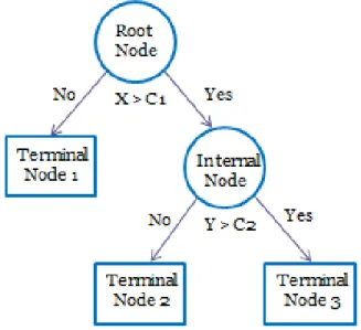
The output of a CART analysis is often displayed in a tree diagram. Figure 1 is a simple illustration. The full dataset is stored in the root node. Cases with variable X greater than C1 are placed to the right branch and cases with X equal to or smaller than C1 are placed to the left branch. The right subset can be divided again, with cases having variable Y > C2 going to the right node and Y <= C2 going to the left. From a regression point of view, all splits beyond the
15 initial split of the root node imply interaction effects (Berk, 2008). In the current example, there is an interaction effect between X and Y so that the influence of Y depends on the value of X. As CART can reuse the same predictor over and over, possibly with different thresholds or cutoff values, there are times when a subsequent partitioning uses the same predictor again, resulting in a more complicated curvilinear function. Berk (2008) named it as a “stagewise” process given that earlier stages will not be revisited once a later stage is set.
CART determines the predicted value based on a majority vote. For a classification tree, the label of the majority group within a terminal node is attached to that node. For example, if 80% of the cases in terminal node 3 are high performers and 20% are low performers, the label of
terminal node 3 is then assigned as “high performers.” When a new case is classified into this node, its predicted group will be “high performer.” For a regression tree, the mean value of the response variable within a terminal node is calculated, and assigned as the predicted value for that group.
After a tree has been constructed, how should its classification or prediction accuracy be evaluated? In general, a training sample is used to develop a tree classifier (i.e., a set of decision rules), and a test sample runs through the classifier to make classifications/predictions. The discrepancy between the predicted and the observed outcomes is used to estimate the level of accuracy, typically indicated by error terms. Two common types of error are usually computed: Overall misclassification error in classification, or overall mean squared error (MSE) in
regression, when the test sample is the same as the training sample used to develop the tree classifier, and the error rate represents how skillful the method has been in fitting the data. This is also called the resubstituition error (Breiman et al., 1984). Generalization error (i.e., cross-validation error, as introduced below) is derived when two different samples, a training sample
16 and a test sample, are used to build and test the tree structure respectively, indicating how skillful the method has been in forecasting (Berk, 2008). For a classification tree, a confusion table, which cross-tabulates the observed and predicted classes, is also critical for evaluating model accuracy from the following perspectives: Type I error (false positive), Type II error (false negative), true positive) and true negative.
Researchers such as Berk (2008) and Strobl, Malley and Tutz (2009) have claimed that the estimated resubstituition error rate is overly optimistic and yields lower than actual error rates. Indeed, Cureton (1950) already pointed out the problem with the resubstitution error in his
classic article. Therefore, when multiple samples are available, or a large sample can be
partitioned into several subsets, it is preferred to use different samples for training and testingto produce a more honest and accurate estimation. In the case when no test sample is available or training sample is limited in size, a widely-used alternative is the k-fold cross-validation procedure (Breiman et al., 1984). According to this method, the original sample is randomly partitioned into k equally sized subsamples. Each time, the combination of the (k -1) subsamples is used to grow the tree, with the one left-out subsample serving as the test sample. This process is then repeated k times until each subsample has been used exactly one time as the test sample. The average classification accuracy (or MSE) across the k results is then used as a single
estimate of cross-validation accuracy. In practice, k usually takes the number of 10. However, if
k equals to N (i.e., total sample size) and each test subsample includes only one case, this cross-validation method is also called the “leave-one-out” estimate.
17 In the past three decades, CART has been used in various scientific areas, such as
genetics, bioinformatics, ecology, finance, mechanical engineering, and neuroscience (e.g., De’ath & Fabricius, 2000; Frydman, Altman, & Kao, 1985; Reibnegger, Weiss, Werner-Felmayer, Judmaier, & Wachter, 1991). Within the broad discipline of psychology, there has been an increasing application of CART for predicting a variety of outcomes, such as violence (Steadman et al., 2000), sexual recidivism (Lloyd, 2008), suicidal ideation (Kerby, 2003), positive and negative affect (Gruenewald, Mroczek, Ryff, & Singer, 2008), perceived life stress (Scott, Jackson, & Bergeman, 2011), college admission (Sah, 1998), and student attrition
(Windham, 1994). Two recent reviews have summarized the application of recursive partitioning methods in psychology (cf. Merkle & Shaffer, 2011; Strobl, Malley, & Tutz, 2009). Despite its popularity in other areas, the application of CART in I/O psychology and management science is rare. In the following section, I review the few studies that have either applied CART, or
compared CART with traditional methods for predicting and/or explaining various organizational behaviors.
One area in I/O psychology that CART has been more frequently considered is to predict and explain employee attrition and job performance. For example, a military study conducted by Stark et al. (2011) compared traditional multiple logistic regression with CART in predicting attrition among first-term enlisted soldiers, and found CART performed slightly better than logistic regression in classifying “stayers” and “leavers”. More importantly, CART was able to uncover nonlinear and configural relationships in the response data and identify different reasons of staying or leaving for soldiers. Gjurich (1999) predicted naval Surface Warfare Officer (SWO) retention level using logistic regression and CART, and identified the reasons for officers’
18 factors for predicting student aviators’ performance in the aviation-training pipeline, including both a categorical outcome of completion/attrition and a continuous outcome of flight school grades. For a non-military setting, Chien and Chen (2008) proposed using a data mining framework to explore the relationship between personnel profiles and work behaviors, and developed decision trees for predicting job performance, retention and turnover reasons based on demographic information and work experience for a high-tech company. Beyond understanding attrition and performance, Keeney, Snell, Robison, Svyantek and Bott (2004) have applied CART to examine patterns of organizational climate and employee personality characteristics associated with three different organizations. Their findings supported the ASA (i.e., Attraction-Selection-Attrition) theory and the presence of a person-environment interaction. CART has also been used to shorten surveys and remove items that do not contribute. For example, in a study conducted by Lee and Drasgow (working paper), a 22-item retention likelihood scale was examined using CART, and the final rule incorporated only 4 useful items that still provided an accurate classification of stayers and leavers. Petway (2010) also applied CART to reduce the length of the Big Five Inventory.
2.3 Comparing CART with Classical Methods
As summarized above, standard parametric models such as linear and logistic regressions fall short in several aspects when used in organizational sciences. The introduction of CART may overcome some of the limitations associated with traditional methods, as described below.
A. Flexibility in handling complex relationships
CART provides researchers with a flexible tool for exploring and exploiting nonlinear and configural relationships as suggested by the data. It is especially suitable for conditions when
19 the researchers suspect that there are complex nonlinear or interaction effects among the
predictors, or between the predictor variables and the criterion, but are not sure about the exact form a priori. In addition, compared to multiple regression’s one-model-fits-all procedure, CART is able to specify an individual equation for each subgroup. In CART, each group of participants can be traced through a series of specific splits and corresponding splitting variables, with each set of splits representing a multiple regression equation. A sample regression equation is
𝑓(𝑋, 𝑍) = 𝛽0+ 𝛽1 [𝐼 (𝑥 ≤ 𝑐1)] + 𝛽2 [𝐼 (𝑥 > 𝑐1 & 𝑧 ≤ 𝑐1)] + 𝛽3 [𝐼 (𝑥 > 𝑐1 & 𝑧 > 𝑐2)] where I represent the indicator function. As noted by Berk (2008, p.104), “In practice, there is no need to translate the partitioning into a regression model; the partitioning results stand on their own as a regression analysis. But if one wishes, the recursive partitioning can be seen as a special form of stepwise regression.” This is especially suitable for identifying subgroups and their corresponding characteristics.
B. Not restricted by parametric assumptions
Another flexibility of CART is that it’s a nonparametric method, which means it does not rely on assumptions about sampling observations from a normal distribution. As discussed above, it can be difficult to meet these assumptions with real data. In situations like these, CART shows superior flexibility in handling a wide variety of data types, without requiring any sort of data transformation prior to analysis. On a related note, extreme responses and outliers are more likely to happen in situations with seriously skewed distributions. While the parametric method can be greatly impacted by outliers if they are not explicitly detected and removed, CART just isolates the outliers into a separate node. Hence, CART’s results are less likely to be affected by extreme responses.
20
C. Ease of handling missing data
When missing values exist for the independent variables, a common procedure embraced by many statistical models is pairwise or listwise deletion, excluding observations with one or more attributes missing. This treatment potentially reduces the amount of information being used for model estimation. Missing values are less of an issue for CART though, because CART examines one variable at a time, so only cases with missing values in that particular variable are temporarily removed, whereas all the other cases are retained for that investigation. When other variables are considered, the observations deleted temporarily in a previous step will be included again. This approach does not involve permanently deleting any cases when developing a
predictive algorithm and therefore maximizes the information being used.
When CART is used to make predictions for a new observation with missing values in any of the splitting variables, a so-called surrogate variable is used to replace the missing variable (Hastie, Tibshirani, & Friedman, 2001). A surrogate variable in CART is the one drawn from the remaining set of variables that most closely mimics or predicts the splits of the primary variable that is missing. This is a much simpler approach than imputing missing values and is preferable when dealing with cases that have partially missing data.
D. White box approach
In most cases, the interpretation of the results derived from a decision tree (i.e., a set of if-then conditional statements) is straightforward and intuitively clear. Any hierarchical nature of the independent variables, their interactions, and their relative importance for different classes, are explicit within the tree structure. This white box approach can be of tremendous help for researchers to uncover the underlying relationships between the predictors and the outcome variable in a more explicit manner, potentially leading to an enhanced understanding and better
21 theory building. For example, each branch in the decision tree can be considered as an individual profile, and the set of predictors and their cut-off values help define the characteristics of that particular profile. Breiman et al. (1984, p.7) noted that “an important criterion for a good classification procedure is that it not only produces accurate classifiers (within the limits of the data) but that it also provides insight and understanding into the predictive structure of the data.” Moreover, a tree diagram is often much easier to comprehend than the regression coefficients for practitioners. This approach is even more desirable when compared to other “black-box”
advanced nonlinear classifiers, such as artificial neural networks (ANN; Bishop, 1995), whose internal patterns are never uncovered.
As a summary, the above section suggested that CART provides a valuable alternative in areas where the traditional regression approach falls short, and offers additional insights that are not otherwise revealed. However, CART is not without its shortcomings. In the following section, I discuss some caveats to note when applying CART.
2.4 Caveats for CART
A. Model Instability
CART may have limitations when stability and generalizability are considered. To make the terminal nodes as homogeneous as possible, CART can construct a very large tree with very few cases in each terminal node, which is usually called overfitting. Overfitting may engender three concerns: it causes the tree structure to be unstable, hard to generalize across samples, and difficult to interpret. Overfitting can be attributed to the following three reasons: first, a small sample size, especially when one or more terminal nodes include only a small number of observations; second, weak predictors, which is usually indicated by heterogeneous terminal
22 nodes; third, highly correlated predictors, which means selecting one of the two competing predictors rather than the other can change a tree structure substantially. To protect the tree from overfitting and strengthen the generalizability of the results, several remedies have been
proposed. The first strategy is to set up a stopping rule, so that the tree will no longer be split after the stopping rule is achieved. A variety of heuristics or options can be used to determine the stopping rule, such as setting up a minimum leaf size (i.e., the number of cases within each node), specifying the homogeneity criteria, or defining the desired number of intermediate steps. The second approach to prohibit CART from constructing a large and unstable tree is through “pruning” (Breiman et al., 1984; Berk, 2008), usually in the backward direction. The underlying mechanism of pruning is to first grow a large tree, then cut off the branches that do not increase predictive accuracy sufficiently. The most widely used pruning strategy is the “minimal cost-complexity pruning” developed by Breiman et al. (1984), which seeks to find a balance between overall misclassification error and tree complexity (i.e., number of terminal nodes) by adding a penalty for complex trees. This process removes weak branches by combining nodes that do not reduce misclassification error sufficiently to justify the extra complexity added. As the value of the penalty parameter can vary across a range, a sequence of optimal trees can be generated. Therefore, a second stage following this pruning step is to carry out a cross validation to select a single best tree. The so called “one standard error rule” (Breiman et al., 1984) is generally used to make this best selection, that is, choose the smallest-sized tree whose cross-validation costs are within the one standard error range of the minimum cross-validation cost. In cases when a large number of predictors are included for a relatively small sample, a more advanced approach to increase model stability and generalizability is through resampling. By resampling, hundreds and thousands of trees are constructed to create a tree ensemble, and the results averaged across
23 the ensemble are then used as the decision rule. The two most popular ensemble methods – Tree Bagging and Random Forests – are discussed below.
B. Model Bias
Another problem with CART is that its “greedy” search mechanism may induce bias in variable selection (Doyle, 1973; Loh, 2002; Loh, 2009): with all other things equal, variables with a larger number of distinct values have a greater chance to be selected as the splitting variables (Hothorn, Hornik, & Zeileis, 2006). For example, a categorical variable X that takes n distinct values can have (2n-1 – 1) binary splits. When n increases, this number grows
exponentially. Thus, a categorical variable with more values has a larger opportunity to be chosen. This selection bias can potentially cause irrelevant variables to be selected, leading to erroneous inferences.
An alternative method for constructing classification and regression trees, called GUIDE (i.e., Generalized, Unbiased Interaction Detection and Estimation), has been developed by Loh (Loh, 2002; Loh, 2009) to overcome the problem of selection bias. The main argument of
GUIDE is that compared to restricting splits to one variable on a single node, one can sometimes gain greater predictive accuracy by splitting on a linear combination of multiple variables. For classification trees, GUIDE involves three steps of chi-square significance tests. Step one is to test for main effects. It performs a chi-square test of independence of each predictor versus the outcome variable and calculates its significance probability. The first split is then based on the most significant variable. When no main effect achieves a specified level of significance, a second step is conducted to test for interaction effects. If an interaction test is significant, a two-level split search for the splitting points is performed. A two-two-level split is needed because the
24 best split of X1 may depend on how X2 is subsequently split; similarly, the best split of X2 may
also need to consider the best subsequent splits of X1. Considering their joint effect, the pair of
variables with the largest chi-square value is then selected. If no test in the first two steps is significant, a third step is performed to test for linear structure. However, Hastie et al. (2001) cautioned that even though this linear combination of splits might improve predictive power, it may hurt interpretability. Therefore GUIDE is limited to two variables at a time when fitting a linear model. With respect to regression trees, GUIDE helps solve three problems: first, it controls for selection bias by applying a chi-square test for signed residuals and a bootstrap calibration of significance probabilities; second, it also includes tests for significant pairwise interactions between regression variables; third, it fits more complex node models (e.g., multiple, stepwise linear, polynomial and ANCOVA) than the piecewise constant model of CART.
GUIDE, although helpful for reducing model bias and uncovering good splits hidden behind interactions, still faces the same problem of instability and lack of generalizability. To address these challenges, two ensemble methods based on the CART algorithm, Tree Bagging and Random Forests, have been proposed.
3. Tree Ensemble Methods
3.1 Tree Bagging
“Bagging,” an abbreviation for “Bootstrap Aggregation,” is built on the idea of bootstrap resampling and majority vote (Breiman, 1996). Take a classification tree as an example. Each time, a random sample of size N is drawn with replacement from the original data to construct a single decision tree without pruning. For each tree, a case is assigned to one of the terminal nodes and the category associated with that node is stored. After repeating this process a number
25 of times, hundreds or even thousands of trees are constructed. Finally, one can count how many trees have classified a case into each category, and assign the class membership based on
majority vote. As for regression trees, the average response across multiple trees is calculated as the predicted outcome for each case. An even more accurate procedure based on bagging is called “out-of-bag” estimation: only observations not included in the bootstrap training sample are used to form the test sample. By aggregating a collection of fitted values, tree bagging is able to compensate for overfitting by reducing random variations and canceling out idiosyncrasy of the training data, which results in a more stable decision algorithm and a more honest estimate of model fit.
Tree bagging, nevertheless, is not without limitations. First, the model averaging process is a black-box approach with limited interpretability. Since bagging involves averaging across a large number of trees, there is no longer a single tree structure for interpretation, and no direct way to relate predictors to the response as in a standard decision tree. The output generated by a bagging procedure is merely the predicted class for each case or the predicted probability of membership in a class, yet the underlying mechanism regarding how each case is assigned is unknown. Another limitation exists when a set of predictors are correlated with each other and the fitted values are not fully independent (Berk, 2008). For example, when two important predictors are highly correlated, the inclusion of one could potentially obscure the effect of the other and prohibit its inclusion, leading to a biased estimate. The introduction of the Random Forests method provides a solution to these problems (Breiman, 2001).
26 Similar to tree bagging, random forests method also leverages the advantage of model averaging by constructing a number of trees from bootstrap samples, and determining the predicted values according to the majority vote (or average). A critical difference between tree bagging and random forests lies in the way they select predictors at each split. For Tree Bagging, all the predictors are examined before each node is split, whereas for random forests, a random sample of the predictors without replacement is taken before each split. This treatment prevents an important predictor from being outplayed by a strong competitor that is highly correlated, and gives each predictor a chance to make an impact in different contexts with different covariates. As a consequence, beyond reducing sampling error, the random forests method also has the following three advantages compared to CART and tree bagging: First, it is able to work with a very large number of predictors. Second, it is preferred for dealing with substantially correlated predictors. Third, it helps further reduce random variance beyond sampling of observations. Therefore, random forests has been claimed to be most suitable for “small n large p problems” (Strobl, Malley, & Tutz, 2009, p. 339) when there are too many predictors with too few
observations. Instead of simultaneously considering all the predictors at the same time, random forests examines a subset of predictors at one time, which is easier to handle. This strategy demonstrates a clear advantage over classical methods such as logistic regression when the number of dimensions is high (e.g., Bureau et al., 2005). Nevertheless, as with bagging, the random forests method is also a black-box approach that is limited in interpretation, lacking a unique tree structure and corresponding statistical functions linking the predictors with the outcome.
27 Estimating the relative contribution of each predictor for overall predictive accuracy usually offers another lens to interpret a model. This is not uncommon given that regression weights are widely considered as the indicator of variable importance. The random forests method provides a mechanism to calculate variable importance that includes two variations. The first one is called raw importance (or Gini importance for classification trees), which evaluates the total decrease in node impurity by splitting on a variable for each tree and then averages over all trees. Every time a split of a node is made on a particular variable, the sum of the split
criterion (i.e., an impurity index such as Gini for classification or MSE for regression) for the two child nodes is less than the parent node. Adding up the impurity decreases for each individual variable over all trees in the random forest gives the estimate of the variable
importance. Although intuitive, this method has been shown to carry forward the bias of a single tree, which favors continuous variables or variables with many categories (Strobl, Boulesteix, Zeileis, & Hothorn, 2007). Thus, it is not recommended in situations when predictor variables vary in their number of categories or scale of measurement. The second approach is called permutation importance (Breiman, 2001). This is achieved by randomly permuting the values of any predictor across all of the observations in the training data set or out-of-bag data set, and comparing the difference in predictive accuracy (i.e., misclassification rate or MSE) between the real data and the permutation data across all trees. If the random permutation of a particular variable substantially decreases the predictive accuracy, then this predictor is considered as a reasonably important one. Otherwise, it is not considered as important. A limitation of the permutation importance method is that it severely over-estimates the importance of a predictor variable if it correlates with other variables (Strobl, Boulesteix, Kneib, Augustin, & Zeileis, 2008).
28 In simple multiple regression, the values of the standardized regression coefficients (or squared standardized regression coefficients) can be used to quantify the importance of different predictors and the strength of the connections between the predictors and the criterion. However, regression coefficients could be seriously distorted given the existence of multicollinearity among predictors. Recently, several comprehensive alternatives based on more solid statistical inferences such as dominance analysis (Azen, Budescu, & Reiser, 2001) and relative weights analysis (Johnson, 2000), have been proposed to overcome the multicollinearity problem. Dominance analysis addresses the problem of correlated predictors by examining the additional contribution of each predictor across all subset of regression models (Azen & Budescu, 2003; Budescu, 1993). Relative weights analysis, on the other hand, adopts a variable transformation approach by creating a set of new predictors that are orthogonal counterparts of the original ones (Johnson, 2000). Although developed based on different statistical rationales, past research has shown that the two methods tend to yield virtually identical results (LeBreton, Ployhart, & Ladd, 2004). However, dominance analysis is less preferred, especially when the number of predictors is large, mainly due to its computational burden (i.e., it computes all possible subsets of
regression models). Indeed, Johnson and LeBreton (2004) noted that dominance analysis can handle no more than 10 predictors at a time. Therefore, relative weights analysis is generally preferred, particularly for high-dimensional data.
Compared to the traditional regression coefficient approach, both random forests and dominance analysis/relative weights are superior when multicollinearity is present (e.g., Bi & Chung, 2011). However, two unique features further differentiate random forests from dominance analysis/relative weights. First, both dominance analysis and relative weights are limited to the first-order linear regression model and do not include any interactive or higher
29 order polynomial effects. This means the variable importance generated from these two
techniques reflects only the “main effects”. Random forests, however, covers the impact of each predictor individually as well as its multivariate interactions with other predictors. Second, the foundational assumption of both dominance analysis and relative weights analysis is that the form and function of the regression model have been correctly specified (Budescu, 1993;
Tonidandel & LeBreton, 2010). This could not be guaranteed particularly with high dimensional data that includes complex interactions. The random forests method offers more flexibility in cases when the regression model is not specified a priori.
4. Comparing Classical Methods, CART, and Random Forests
4.1 Brief Review of Several Classical Methods
Two of the most commonly adopted modeling methods for classification problems are Fisher’s discriminant analysis (DA) and logistic regression (LR). The underlying mechanism of discriminant analysis is to find a linear combination of a set of continuous predictors that best differentiates two or more classes of objects or events based on ordinary least squares (OLS). Discriminant analysis formulates a function that predicts the probability of an individual falling into each category, and then assigns the group membership based on the highest probability. When group variances are equal, linear discriminant analysis (LDA) is used; otherwise, quadratic discriminant analysis (QDA) is applied. However, DA is based on OLS that assumes normal distributions of the error variances. When this requirement is not satisfied and the dependent variable is a binary outcome, logistic regression (LR) is usually preferred for modeling the binomial distribution. LR is a special form of the generalized linear model with the link function being a log transformation of the odds ratio (i.e., the probability that an observation belongs to
30 one category divided by the probability that it falls into the other category), which is often called a logit function, as shown in the formula below. It describes how the probably of a binary
outcome is related to a linear combination of the predictor variables (Hosmer & Lemeshow, 1989). Unlike DA that uses OLS, LR obtains parameter estimates through maximum likelihood estimation. logit (𝜋(𝑥𝑖)) = log ( 𝜋(𝑥𝑖) 1 − 𝜋(𝑥𝑖)) = 𝛼 + 𝛽1 𝑥1𝑖+ … + 𝛽𝑗 𝑥𝑗𝑖 + 𝑒𝑖 or alternatively in terms of 𝜋(𝑥𝑖): 𝜋(𝑥𝑖) = exp{𝛼 + 𝛽1 𝑥1𝑖+ … + 𝛽𝑗 𝑥𝑗𝑖 + 𝑒𝑖} 1 + exp{𝛼 + 𝛽1 𝑥1𝑖+ … + 𝛽𝑗 𝑥𝑗𝑖+ 𝑒𝑖}
When the response variable is a continuous numerical one, multiple linear regression, which is another form of generalized linear model with the link function being “identity,” is most commonly used (formula shown below):
𝑌𝑖 = 𝛼 + 𝛽1 𝑥1𝑖+ … + 𝛽𝑗 𝑥𝑗𝑖+ 𝑒𝑖 where 𝑒𝑖 ~ 𝑁 (0, 𝜎2) and independent.
4.2 Comparing Classical Methods, CART, and Random Forests
A number of previous empirical and simulation studies have compared the predictive accuracy of CART and the above mentioned classical methods. Results from empirical studies based on single dataset have been conflicting. For instance, several studies have found that traditional methods such as LDA, QDA, and LR performed comparably or better than CART (Arminger, Enache, & Bonne, 1997; Dudoit, Fridlyand, & Speed, 2002; Preatoni et al., 2005;
31 Ripley, 1994; Williams, Lee, Fisher, & Dickerman, 1999), whereas other studies (e.g., Grassi, Villani, & Marinoni, 2001) reported that CART provided higher classification accuracy than LDA. These conflicting results might be attributed to the idiosyncratic nature of the sample being used. A couple of simulation studies suggested that certain data and model distribution characteristics had differential impacts on the classification accuracy of traditional methods and CART. For example, Finch and Schneider (2006, 2007) conducted two Monte Carlo simulations that compared the cross-validated misclassification accuracy of LDA, QDA, LR, and CART under a variety of simulated conditions. Their results indicated that when the parametric assumptions such as normal distribution and equal covariance matrices of the two groups were met, LDA and LR performed as well as QDA and all were slightly better than CART. However, when the two groups’ covariance matrices are not equal, regardless of the underlying distribution of the predictors, QDA and CART consistently outperformed LDA and LR. The more unequal, the better QDA and CART performed. They also found a significant main effect of the group size ratio: when the two groups were extremely unequal in size (e.g., 10:90), the
misclassification rate was consistently higher for the smaller group regardless of data distribution, sample size, or the modeling method being used. However, Finch and Schneider (2006) showed that CART did offer some buffering effects in situations like that, showing a slightly lower misclassification rate for the smaller group and a higher classification error for the larger group. These authors noted that one limitation of their simulations was that the interaction effects among the variables were not considered at all. Therefore, a more comprehensive simulation was conducted to extend the comparison (Holden, Finch, & Kelly, 2011). Holden et al. (2011)
showed that when the simulated models included interactions, linear models such as LDA, QDA, and LR consistently had difficulty in obtaining accurate classification, whereas CART always
32 produced the greatest accuracy. The superiority of CART was particularly notable when the relationship between group membership and the predictors was complex and nonlinear. Similar conclusions were also supported by several other simulation studies regarding the impact of nonlinear relationships (Curram & Mingers, 1994; West, Brockett, & Golden, 1997), with the results showing that LDA and LR performed as well as more advanced alternatives such as classification trees under linear conditions, but were not as effective when the relationships between the predictors and the criterion measure were nonlinear.
Prior simulation studies comparing CART with traditional multiple linear regression (MLR) for predicting continuous outcomes have demonstrated similar results to that when predicting a categorical criterion. Breiman et al. (1984) conducted several simulation and empirical studies comparing regression trees with linear regression, and concluded that regression trees could be much more accurate for nonlinear problems, but tended to be less accurate when the problem followed a good linear structure. Garson (1998) also showed that linear models such as MLR performed poorly for prediction when a number of interactions existed among the predictor variables, based on a Monte Carlo simulation. Empirical evidence showed that CART performed comparable or slightly better than multiple linear regression in terms of predictive accuracy (Finch et al., 2011; Kerby, 2003; Fu, Anderson, Courtney, & Hu, 2007), yet demonstrated additional advantages in other areas: CART displayed lower RMSE and higher R2 results than did MLR, and offered cutoff scores to aid decision making in applied settings.
Unlike comparisons between CART and traditional methods which are bounded by sample and model characteristics, studies comparing random forests with other methods have generally shown that random forests possess higher levels of predictive accuracy than other
33 classical methods or a single decision tree. Halstead (2006) compared linear regression with random forests and two alternatives and found that random forests best predicted military recruiter’s job performance while linear regression yielded the worst prediction. Based on the random forests variable importance selection mechanism, Halstead (2006) identified the best subset of features out of 260 predictors that produced the best model generalization. Sut and Simsek (2011) compared CART, random forests, and a set of other regression methods for predicting mortality in head injuries, and showed better performance for random forests than CART based on both overall accuracy and area under the ROC Curve. Loh (2009) also conducted a set of simulation studies comparing ensemble tree methods with several single-decision-tree methods such as CART and GUIDE, and found that in general, ensemble methods fit better than any of the single-tree methods, and random forests was the best for most samples. In addition to superior predictive accuracy, the random forests method also excels at finding important predictors. A simulation study conducted by Eliot (2011) showed that when there was no structure among the predictors, random forests performed better than LR and CART at finding the order of variable importance, especially when predictors were not highly correlated. However, when the data was structured in the way that one variable was only predictive of the outcome within a level of another variable, CART and LR described the data better than random forests. Eliot (2011) suggested that each method may be best suited for certain types of data and distributions, and combining them may provide additional insights.
5. The Current Study
Given previous theoretical and empirical evidence, it is expected that CART would outperform traditional classification and regression methods, such as DA, LR or MLR, when nonlinear, interactive, or complex configural relationships exist in the data. The classification
34 accuracy may also vary depending on parameters such as group size ratio (Finch & Schneider, 2006, 2007; Perlich, Provost, & Simonoff, 2003). However, although random forests is expected to perform better than CART and other traditional methods in a variety of conditions, there is a lack of simulation research comparing random forests with CART and other methods under nonlinear data structure or various group size ratios. As a consequence, the first purpose of the current study is to replicate and extend previous simulations by comparing CART and random forests with classical methods such as logistic regression, linear and quadratic discriminant analysis, and multiple linear regression for predicting both categorical and continuous outcomes under a variety of manipulated conditions. In addition to the set of parameters examined before, I also included some other factors that have theoretical or empirical relevance with organizational research. Using a series of Monte Carlo simulations, the first two studies examined the
methodological strengths and weaknesses of CART and random forests compared to the set of commonly used regression-based methods, particularly in the context of organization research.
The second goal of the current research was to illustrate the empirical application of CART and random forests using real data, comparing their predictive accuracy with the same set of traditional methods for addressing employee turnover problem (a binary outcome) in Study 3 and job performance (a continuous outcome) in Study 4. The aim of these two studies was to offer practical guidance regarding how CART and random forests could be combined to enhance both model prediction and interpretation.
In a summary, the current paper provides an exposition and new findings regarding recursive partitioning methods for the researchers in the field of organizational sciences, and offers some empirical suggestions about when and how these methods should be applied.
35 CHAPTER 2: METHOD
STUDY 1
In Study 1, a Monte Carlo simulation was carried out to systematically compare the two decision tree methods, CART and random forests (RF), with three traditional classification methods: logistic regression (LR), linear discriminant analysis (LDA), and quadratic
discriminant analysis (QDA). In particular, the current study aimed at exploring if and when the decision tree methods were superior to the traditional methods. The manipulated parameters were selected to cover a variety of characteristics associated with the sample (base rate), distributions (level of skewness), relationships within the set of predictors (multicollinearity), and the relationships between the predictors and the outcome variable (variance explained and data complexity). These parameters were chosen based on their theoretical and practical
relevance to personnel selection research (Aguinis, Culpepper, & Pierce, 2010; Bobko, Roth, & Potosky, 1999; Finch, Edwards, & Wallace, 2009).
Personnel selection was of particular interest in the current paper because, given the high-stakes context of personnel selection, predictive accuracy is usually the foremost concern – even a small improvement in predictive utility can lead to a substantial monetary saving, such as reducing training costs (White, Nord, Mael, & Young, 1993) or increasing return on investment (ROI). In addition, understanding how predictors and criterion are related could assist personnel psychologists to develop better selection decisions. Note that sample characteristics and sample size were beyond the scope of the current study. This is because previous literature (Fan & Wang, 1999; Lei & Koehly, 2003) found that sample size was not a significant factor in differentiating CART from LR or other traditional methods. Thus, the sample size was fixed to 1, 000 in the current study to make sure that when the base rate was set to be relatively small, there would be