Archive University of Zurich Main Library Strickhofstrasse 39 CH-8057 Zurich www.zora.uzh.ch Year: 2017
An agent-based simulation of the stolper–samuelson effect
Meisser, Luzius ; Kreuser, C Friedrich
Abstract: We demonstrate that agent-based simulations can exhibit results in line with classic macroe-conomic theory. In particular, we present an agent-based simulation of an Arrow–Debreu economy that accurately exhibits the Stolper–Samuelson effect as an emergent property. Absent of a Walrasian auc-tioneer or any other central coordination, we let firm and consumer agents of different types interact in an open, money-driven market. Exogenous preference shocks result in price and wage shifts that are in accordance with the general equilibrium solution, not only qualitatively but also quantitatively with high accuracy. Key to this achievement are three independent measures. First, we overcome the poor input synchronization of conventional price finding heuristics of firms in agent-based models by introducing sensor prices, a novel approach to price finding that decouples information exploitation from information exploration. Second, we improve accuracy and convergence by employing exponential search as exploration algorithm. Third, we normalize prices indirectly by fixing dividends, thereby stabilizing the system’s dynamics.
DOI: https://doi.org/10.1007/s10614-016-9616-x
Posted at the Zurich Open Repository and Archive, University of Zurich ZORA URL: https://doi.org/10.5167/uzh-131315
Journal Article Accepted Version Originally published at:
Meisser, Luzius; Kreuser, C Friedrich (2017). An agent-based simulation of the stolper–samuelson effect. Computational Economics, 50(4):533-547.
Electronic copy available at: http://ssrn.com/abstract=2794828
(will be inserted by the editor)
An Agent-Based Simulation of the Stolper-Samuelson
Effect
Luzius Meisser · C. Friedrich Kreuser
Received: date / Accepted: date
Abstract We demonstrate that agent-based simulations can exhibit results in line with classic macroeconomic theory. In particular, we present an agent-based simulation of an Arrow-Debreu economy that accurately exhibits the Stolper-Samuelson effect as an emergent property. Absent of a Walrasian auc-tioneer or any other central coordination, we let firm and consumer agents of different types interact in an open, money-driven market. Exogenous prefer-ence shocks result in price and wage shifts that are in accordance with the general equilibrium solution, not only qualitatively but also quantitatively with high accuracy. Key to this achievement are three independent measures. First, we overcome the poor input synchronization of conventional price find-ing heuristics of firms in agent-based models by introducfind-ing sensor prices, a novel approach to price finding that decouples information exploitation from information exploration. Second, we improve accuracy and convergence by employing exponential search as exploration algorithm. Third, we normalize prices indirectly by fixing dividends, thereby stabilizing the system’s dynamics.
Keywords Computational economics · agent-based economics · price finding·price normalization·sensor prices·system dynamics
1 Introduction
Agent-based simulations are complex, often chaotic systems. As such, they ex-hibit rich dynamics that are hard to achieve with traditional means. However, these rich dynamics can be a curse rather than a blessing as they can lead to Luzius Meisser University of Zurich Tel.: +41-76-558-27-12 E-mail: [email protected] C. Friedrich Kreuser University of Stellenbosch
Electronic copy available at: http://ssrn.com/abstract=2794828
arbitrary, unverifiable results. This insight lead us to build a stable, verifiable agent-based model instead, with equilibria that are in line with classic the-ory. In particular, we implemented a minimal agent-based simulation of the Stolper-Samuelson effect (Stolper and Samuelson, 1941) in an Arrow-Debreu economy with profit-maximizing firms (Arrow and Debreu, 1954). The choice of the Stolper-Samuelson effect is rather random and of secondary importance. The prime achievement of this paper lies in the introduction of methods to enable the simulation of a classic result with unprecedented accuracy.
There are a number of agent-based projects that aim at comprehensively modeling a large-scale economy, examples being the Eurace project by Deis-senberg et al (2008), the family of models by Gatti et al (2011), and the Jamel framework by Seppecher (2012). Due to their complexity, it is non-trivial to rigorously test them. In contrast, our simulation focuses on a single, well-defined effect, allowing for exact quantitative verification. In this regard, we follow the footsteps of authors such as Brock and Hommes (1998), Gintis (2007), or LeBaron (2001), who encourages benchmarking agent-based models with classic equilibrium results. Implementation-wise, our model most closely resembles that of Wolffgang (2015) with its emphasis on applying best prac-tices from software-engineering. To our knowledge, Wolffgang’s model is the first to apply the exponential search algorithm discovered by Bentley and Yao (1976) to price finding, an idea we adopt and adjust.
While exponential search helps to achieve faster convergence and better accuracy, it does not address input synchronization. Input synchronization being hard to achieve in price-driven markets has also been observed by firm theorists Milgrom and Roberts (1994). For firms depending on multiple per-ishable input goods (in our model different types of man-hours), it is essential that all their bids succeed. With Cobb-Douglas production, failing to acquire one of the input goods already leads to a total loss of production. We improve input synchronization by introducing sensor prices. Furthermore, causal loop diagrams – a tool from system dynamics – are used to identify the method of normalizing prices indirectly by fixing dividends as a more stable choice than the usual method of normalizing a randomly chosen price directly. While irrelevant in static equilibrium theory, the choice of how to normalize prices decidedly impacts the dynamics of the simulation. Together, these three mea-sures enable the emergence of the theoretically expected equilibrium with high accuracy.
Section 2 specifies the rather unspectactular general-equilibrium version of our model. In section 3, the fundamental mechanisms of the agent-based model are described and analyzed. Results are presented in section 4. It turns out that – within a certain parameter space – our agent-based simulation is stable, accurate, and fast. Finally, we conclude with section 5.
2 General Equilibrium Model
The Stolper-Samuelson theorem states that if the price of a good rises, then the input factor most intensively used in its production should rise along with it.1(Stolper and Samuelson, 1941) Thus, an economy with at least two output goods and two inputs factors is needed. For illustrative purposes, we call the two types of goods pizza and fondue. They are produced by according types of firms, pizzeria and chalet. There are also two types of inputs: Italian and Swiss man-hours, whereas Swiss man-hours are more intensively used for the production of fondue and Italian man-hours are more intensively used for the production of pizza. Both, the Swiss and the Italian consumers, have the same preferences. By default, they both prefer pizza. The consumers are endowed with 24 man-hours per day, part of which they sell on the market, buying pizza and fondue in return. Exogenous preference shocks are used to trigger price shifts and their effect on wages is observed. As these shocks come unexpected to the agents and the economy is static otherwise, intertemptoral considera-tions are unnecessary and each configuration can be solved as an independent equilibrium in an Arrow-Debreu spot market.
Consumers derive utility from a log-utility function with consumed pizza, fondue and leisure as weighted inputs. The utility function of a single consumer of typec∈ {Italian, Swiss}is:
Uc(xc,pizza, xc,f ondue, hc) =αln(xc,pizza+1)+βln(xc,f ondue+1)+γln(25−hc)
withα,β, andγquantifying the preferences for each consumable,hc denoting
the man-hours sold on the labor market, and for examplexItalian,f onduebeing
the amount of fondue consumed by the Italian consumers. Note the increments +1 for each consumable to ensure that utility is always positive. Without them, a single consumer failing to acquire one of the inputs on a single day would suffice to drag the average experienced utility for all consumers down to−∞, thereby spoiling average utility as a benchmark for the simulation.
Consumerscmaximize utility subject to their budget constraint
wchc+dc =ppizzaxc,pizza+pf onduexc,f ondue (1)
with hourly wagewc, dividend incomedc, and pricesp.
Given prices, firms produce to maximize profits, which they distribute evenly to the consumers as dividend. They have a Cobb-Douglas production function with decreasing returns to scale in order to rule out monopolistic equilibria. Pizzerias (piz) have production function (2), chalets (cha) have production function (3).
xpizza(hItalian,piz, hSwiss,piz) =A h δhigh Italian,pizh
δlow
Swiss,piz (2)
1 Originally, the theorem was only shown to hold for two inputs and two outputs, with constant returns to scale and constant supply of inputs. While Jones and Scheinkman (1977) generalized it to larger number of inputs and outputs, the Stolper-Samuelson effect is not guaranteed to appear when returns to scale are not constant (Jones, 1968) or supply of inputs is variable (Martin, 1976), both of which is the case in our model. Nonetheless, the effect is present in the discussed settings thanks to their parametric symmetry.
xf ondue(hItalian,cha, hSwiss,cha) =A hδItalian,chalow h δhigh
Swiss,cha (3)
Parameters A, δlow, and δhigh are constant, with δlow < δhigh, and δlow+
δhigh<1.0. The profit function of a pizzeria is provided later as equation (4).
In the agent-based simulation, each of the hundreds of consumers and firms acts on its own. In the general equilibrium case, each agent type is repre-sented by one representative agent whose consumed and produced quantities are scaled to the actual number of agents.
A script to calculate the general equilibrium solution is provided as sup-plement (see section 4.3).
3 Agent-Based Model
Instead of explicitely imposing equilibrium conditions, agent-based models del-egate that work to market forces, hoping for equilibria to emerge naturally.
Our simulation approaches its equilibrium over the course of many iter-ations (days), forming a sequence of reopening spot markets with nightly production. Money is introduced as a store of value and to facilitate trad-ing. According to Feldman (1973), the presence of money in an Arrow-Debreu economy guarantees that bilateral trading suffices to reach pareto-efficiency, whereas in general, atomic trades involving three or more agents might be necessary.
Our consumer and firm agents have the same utility and production func-tions as in the general equilibrium model. Preferences are set per consumer type and production parameters per firm type. However, each individual agent has its own stocks of money, pizza, fondue and man-hours, whereas Italian and Swiss man-hours are traded as distinctive goods. Furthermore, each firm has its own price beliefs at which it posts offers (bids and asks) to the market. All quantities are continuous.
3.1 Sequence of Events
Like the real world, agent-based models do not permit instant market clear-ing. Instead, trades and other events happen in chronological order. Circular dependencies are broken apart. For example, firms in our model cannot sell output goods they have not produced yet, requiring them to sell yesterday’s production today and today’s production tomorrow.
Furthermore, the dynamics of a simulation are affected by causality, which is irrelevant to the equilibrium solution. For example, the equationd=πdoes not distinguish cause and effect. But in the simulation, it makes a difference whether dividends determine profits or profits determine dividends. Here, the sequence of events plays a pivotal role.
In our model, each firm is endowed with 1000$ before the first day begins. Then, days are structured as follows:
1. Consumers are endowed with 24 man-hours each.
2. Firms distribute excess cash as dividends. Excess cash is defined in absolute terms, e.g. max(0, cashpiz,17−800) for pizzeria number 17. This can be seen as an elaborate way of normalizing prices and is further explained in section 3.2.
3. Firms post asks to the market, offering yesterday’s production in accor-dance with their individual price beliefs; for example ”we sell 79 pizzas for 7.30$ each”. The market can be seen as a passive bulletin board, as described by Eidson and Ehlen (2013).
4. Given their price beliefs, firms calculate maximum profits and set according budgets for each input good. Based on these budgets, they post bids in the form of limit-orders to the market, for example ”we buy up to 50 Swiss man-hours for 13$ each”.
5. In random order, consumers enter the market and optimize their utility given the offers they find, selling man-hours and buying pizza and fondue. 6. The market closes and each firm updates its price beliefs based on whether
the relevant orders were filled or not.
7. Firms use all acquired man-hours to produce the outputs to be sold tomor-row. Unsold outputs are carried over to the next day, whereas unused man-hours cannot be stored. In equilibrium, all money resides with the firms again at this point in time, although not necessarily equally distributed.
3.2 Dynamics and Price Normalization
Due to their complexity, it is often hard to tell in advance whether agent-based models are attracted to the desired equilibria or not. One method of classifying models as stable or unstable is to calculate their Lyapunov expo-nent, as mentioned by Axtell (2005) and described by Hommes (2013). For our purposes, the much simpler causal loop diagrams suffice, which we use in ac-cordance with the guidelines of Kim (1992). They help analyzing the model’s dynamics and substantiate why it is advisible to choose other methods of price normalization in the simulation than what is usually done analytically.
Causal loop diagrams allow to quickly reach a qualitative judgement on whether a feedback loop is reinforcing (unstable) or balancing (stable). Unde-sired reinforcing feedback loops are colloquially calledvicious cycles. Causal loop diagrams visualize system variables as nodes in a directed graph. Edges are either labeled with a + or−, depending on whether an increase of the orig-inating variable leads to an increase or decrease of the target variable. In such graphs, feedback loops passing an even number of minusses are reinforcing, while those with an odd number are balancing.
Figure 1 shows the causal loop diagram for a firm’s price belief regarding the output good. A firm that believes it can sell at a higher price will try to produce more, thus increasing its production target. A higher production target subsequently results in a higher actual production and a larger stock of goods to be sold. However, the higher the stock, the less likely it becomes to
Production target Stock Probability of selling whole stock Output price belief
+
−
+
+
−
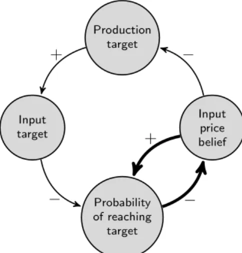
Fig. 1 The causal loop diagram for a firm’s output price belief has two balancing feedback loops. Production target Input target Probability of reaching target Input price belief
+
−
−
−
+
Fig. 2 Causal loop diagram for input price beliefs, also containing two balancing feedback loops.
fully sell it on the market. Additionally, trying to sell the stock at a higher price also leads to a reduced sale probability. Applying one of the belief adjustment heuristics discussed in 3.3, a high sale probability results in a higher price belief, thereby closing the two loops. Note that both loops are balancing, and thus stabilizing the system.
The price dynamics for the input good are similar and illustrated in fig-ure 2. Here, a low price belief leads to an increased production target. A firm should produce more as its input factors are getting cheaper. The higher pro-duction target calls for acquiring larger input quantities, which in turn makes a successful purchase of that increased input amount less likely. A decrease in
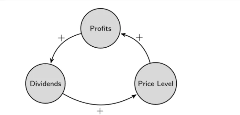
Profits
Dividends Price Level
+
+
+
Fig. 3 A vicious cycle with self-reinforcing inflation or deflation.
that probability pushes the price belief upwards via the algorithms specified in section 3.3, thereby closing the outer loop. The inner feedback loop connects the input belief directly with the probability of reaching the purchase target, as offering a higher price makes it more likely that enough willing workers are found.
In equilibrium models, the price of the first output good is usually nor-malized to one, thereby determining the nominal price level. However, doing the same in an agent-based simulation is not advisable as it can reduce the stability of the system. For example, imposing ppizza = 10$ would interrupt
that price’s two balancing feedback loops, thereby leaving all the work of ap-proaching the equilibrium to the input side and to the other firm types. This is analogous to a central bank trying to control price levels by setting the price of bread to one and waiting for all other prices to adjust accordingly.
While it is possible to not normalize prices at all and let the simulation settle on a random price level as later shown in figure 11, there is an alternative way of price normalization that comes with the benefit of additionally stabiliz-ing the system. Instead of basstabiliz-ing dividends on profits, we let firms distribute all their cash holdings above a given threshold as dividends. Observing that all money resides with the firms at the end of each day, and setting the threshold low enough, this policy effectively makes daily dividends a constant.2 Besides binding nominal prices to money supply, this policy also improves stability by breaking the vicious cycle of dividends, profits, and prices from figure 3.
πpiz =income−cost=ppizzaxpizza−
X
c
wchc,piz (4)
This vicious cycle can also be understood analytically. First, nominal profits rise with the price level, as can be intuitively seen from the profit function (4) of the pizzeria. When prices and wages are increased by a constant factor, equilibrium profitsπpiz grow by the same factor. Second, dividends are
usu-ally set equal to profits, extending the proportional dependency to dividends. 2 With thresholdτ, total dividends ofnfirmsfwith cashcfeach aredtot=P
f(cf−τ) =
P
Third, the vicious cycle is closed by recognizing from the consumer’s budget constraint (1) that equilibrium prices are proportional to the consumer’s cash holdings at the beginning of the day,3
which happens to consist entirely of dividends in our model.
By effectively making daily dividends a constant, this vicious cycle is bro-ken and the simulation stabilized.
3.3 Exponential Search
In agent-based simulations with endogenous price-discovery, firms typically have price-beliefs that are updated heuristically, based on whether a market offer based on the current price belief was filled. For example, a pizzeria that offered 200 pizzas for 11$ each will adjust the price upwards if it succeeds in selling them and will adjust the price downwards if not. The case of a partially sold inventory can be neglected as this only happens rarely with large enough numbers of competing firms.
Conventional Methods Many simulations adjust prices by a certain percent-age, i.e.pt+1= (1±s)pt, examples being Gintis (2007), Catalano and Di Guilmi
(2015) and Gatti et al (2011). One shortcoming of this approach is that it is not symmetric. Increasing a pricepand decreasing it again counter-intuitively leads topt+1=pt(1 +s)(1−s)6=pt.
To ensure symmetry, one should multiply or divide by a constant factor instead, i.e. pt+1 = pt(1 +s) or pt+1 = pt/(1 +s). However, this approach
can still suffer from coarse granularity and a biased average. To see this, first note that in a situation with stable prices, symmetry dictates beliefs to be too high and too low equally often. If this was not the case, price beliefs would move over time, contradicting the assumption of stable prices. As an example, assume a market price of 101$ and an adjustment factor of (1 +s) = 1.05. Starting with 100$, a firm’s price belief will alternate between 100$ and 105$. The average price belief among the firms will thus be around 102.5$, above the market price of 101$. Riccetti et al (2014) overcome this bias through randomization. For example, a newsrand could be chosen uniformly for every
step, withsrand∼U(0,2s).4
When chosing the adjustment factor, there is a trade-off between speed of convergence and accuracy. A large factor lets the price belief approach the mar-ket price faster, while a small factor allows for higher accuracy. Generally, the number of steps it takes to converge is linear in the relative logarithmic distance between price belief and market price, i.e. it is inO(|logf(pbelief/pmarket)|). In
practice, it can take longer depending on the competitive dynamics between firms.
3 A quick path to this insight is to imagine the consumer being endowed with one gold nugget of market pricedinstead of dividendsd. This yields the same outcome, yet transforms
dinto a price that must be – like every price – proportional to the general price level. 4 To be precise, Riccetti et al. randomize the percentage approach, i.e.pt
+1= (1±s)pt withsuniformely distributed, leading to a forth variant not discussed here.
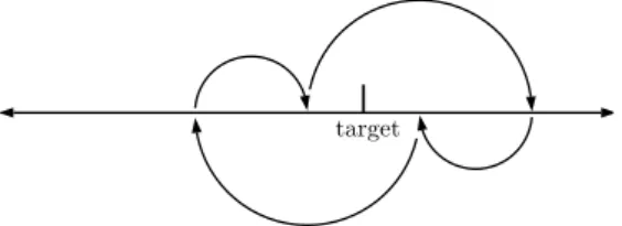
target start
Fig. 4 Adapting price beliefs with exponential search: increasing the adjustment factor after every second step in same direction, decreasing on turns
target
Fig. 5 Trap: no convergence when increasing the adjustment factor too early
Exponential Search Exponential search is an algorithm that efficiently solves the unbounded search problem by dynamically adjusting its step size. It finds a target element in an unbounded list in logarithmic time, i.e. inO(log(d)) with d being the number of steps it would take with a linear search. Exponential search was first described by Bentley and Yao (1976) and is well-known among computer scientists. Since the firm’s problem of finding a market price is also a search in an unbounded, one-dimensional space, employing exponential search is a natural choice.
Classic exponential search doubles the adjustment factor on every step un-til it passes by the target value and then switches into bisection mode. To allow for dynamics, Wolffgang (2015) suggests to generally increase the ad-justment factor on steps in the same direction as before and to decrease it on turns. Unfortunately, this can lead to cycles, thereby preventing convergence, as shown in figure 5. We address this by only doubling after every second step in the same direction, leading to the algorithm illustrated in figure 4. Fur-thermore, doubling and halving might be too aggressive, potentially causing or amplifying oscillations. Wolffgang applies a factor of 1.1, a value which we adopt.
All these choices are methodologically motivated. We choose exponential search with these parameters because it helps the simulation at the macro-level in finding the theoretic equilibrium more quickly and accurately, and sometimes also to catch up with shocks that would escalate with conventional adjustment methods. There are no behavioral observations or other micro-foundations behind these choices other than that they work well.
Unfilled orders
Filled orders
Highest paid price
Fig. 6 Typical price adaption heuristics lead to filled orders only half of the time, alternating between a price below and above what the market can bear.
3.4 Sensor Prices
In equilibrium, half of the offers will not fill when adjusting symmetrically up- and downwards as described in the previous section. In particular, firms with multiple, perishable input factors suffer from poor input synchronization, a phenomenon described by Milgrom and Roberts (1994). A pizzeria with Cobb-Douglas production that fails to either acquire Swiss or Italian man-hours, will produce nothing at all on that day. Coase (1937) suggests to address market frictions by introducing long-term contracts, which is also the preferred solution in reality when acquiring man-hours. Customer loyalty can also help, as Rouchier (2013) demonstrates with an agent-based simulation. To preserve the elegance of a sequence of independent spot markets, we decided to apply a new method, which we callsensor prices.
Normally, when posting an order to the market, agents face a trade-off between information exploitation and information exploration, as Tesfatsion (2006) points out. In the case of a sale, they want to maximize revenue, but also collect as much information as possible about the optimal price level. These two conflicting goals can be disentangled by posting two seperate offers, one that maximizes revenue and one to find out what prices the market can bear.
Figure 6 illustrates how only every second order is filled when using typical price adaption heuristics. Figure 7 shows how sensor prices can improve the situation. The sensor offer constantly tests the price level and adjusts itself accordingly. It uses a fractionθs of the total sales volumes, whereas the
ma-jority of the output is sold at a close, yet safe, relative distanceθd, leading to
prices pvolume =psensor/(1 +θd) when selling and pvolume =psensor(1 +θd)
when buying. For simplicity, we imposeθs=θd=θ.
In order to find the right distance between sensor price and volume price, their relative distanceθd is dynamically adapted. Whenever the volume offer
fills, it is cautiously moved a little closer to the sensor offer, with θt+1 = θt/1.005. However, if it does not fill, distance is doubled to keep the risk of
repeated failures low, i.e. θt+1 = 2θt. With this strategy, one can expect the
ratio of failures to be 1/log1.005(2) < 1%. These parameters have been set intuitively by trial and error, without further analytic evaluation.
There is no real-world economic intuition behind sensor prices other than the observation that firms sometimes perform price tests. We use sensor prices
Sensor prices
Large orders in safe distance Highest paid price
Fig. 7 With sensor prices, only a small fraction of volume is sacrificied for price exploration, whereas the bulk can reliably drive revenue.
because they work well for firms in a sequential Arrow-Debreu economy. Most importantly, they help firms to synchronize their inputs and thereby lift the whole simulation closer to the efficient equilibrium at the macro-level. In man-agement science, sensor prices would likely be considered a form of dynamic pricing, as for example researched by Elmaghraby and Keskinocak (2003). However, they differ insofar as dynamic pricing is primarily concerned with price discrimination, which is the art of selling the same product at different prices depending on the consumer, while sensor prices are tailored towards information exploration in an open market with indistinguishable consumers.
4 Result
The agent-based simulation exhibits the Stolper-Samuelson effect as an emer-gent property with high accuracy for a wide range of parameters. Within the parameter space
0.1≤δ≤0.6 0.1δ≤δlow≤0.5δ 1≤α≤9
the average deviation from the efficient solution is 0.03% with a median of 0.015% and a few outliers near the boundaries of the aforementioned parameter space. This high level of accuracy is only achieved when employing all the three discussed techniques in combination. For returns to scaleδ≥0.6, the stability of the simulation detoriates quickly, an issue which would be worthwhile to address in future research.
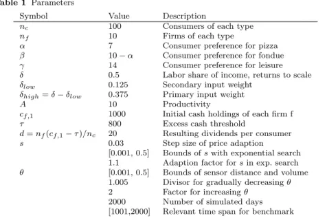
The default configuration assigns the parameter values shown in table 1. No exogenous shocks are included as long as we are only concerned with the asymptotic outcome, which does not depend on the point in time the relevant parameter values are set.
4.1 Algorithm Comparison
Table 2 compares the accuracy of exponential search to those of conventional adaption algorithms, with exponential search being the clear winner.
Gener-Table 1 Parameters
Symbol Value Description
nc 100 Consumers of each type
nf 10 Firms of each type
α 7 Consumer preference for pizza
β 10−α Consumer preference for fondue
γ 14 Consumer preference for leisure
δ 0.5 Labor share of income, returns to scale
δlow 0.125 Secondary input weight
δhigh=δ−δlow 0.375 Primary input weight
A 10 Productivity
cf,1 1000 Initial cash holdings of each firm f
τ 800 Excess cash threshold
d=nf(cf,1−τ)/nc 20 Resulting dividends per consumer
s 0.03 Step size of price adaption
[0.001, 0.5] Bounds ofswith exponential search 1.1 Adaption factor forsin exp. search
θ [0.001, 0.5] Bounds of sensor distance and volume
1.005 Divisor for gradually decreasingθ
2 Factor for increasingθ
2000 Number of simulated days
[1001,2000] Relevant time span for benchmark
Table 2 Accuracy of price adaption methods in a typical simulation run in comparison to the equilibrium benchmark. Exponential search scores consistently well, whereas the perfor-mance of the other methods can deviate substantially. In this run, the constant percentage method got particularly unlucky.
Method ppizza
pf ondue Error
ppizza
wSwiss Error xpizza Error
Constant percentage 1.5388 10.3% 2.3942 9.87% 544.7 14.80%
Constant factor 1.7188 0.19% 2.6647 0.3% 630.2 1.42%
Randomized factor 1.7244 0.52% 2.6047 1.95% 589.8 7.74%
Exponential search 1.7153 0.01% 2.6572 0.02% 639.1 0.03%
Benchmark 1.7155 2.6566 639.3
ally, prices of goods tend to be more accurate than wages and trading volume tends to be the least accurate. The measured prices are volume-weighted av-erages. This increases accuracy a little as mispricings normally also come with reduced trading volumes, and thus have a lower weight in the metric. Surpris-ingly, increasing the number of agents per type does not necessarily lead to more accurate results. Intuitively, one would expect consistently higher accu-racy with larger populations due to the law of large numbers. Investigating the driving forces behind these differences might be a topic for future research.
4.2 Dynamics
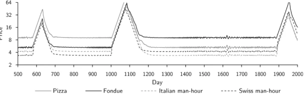
To investigate the dynamic behavior of the simulation, a preference shock is introduced on day 1001. That day, consumers wake up suddenly preferring fon-due over pizza, with swapped preference parametersαandβ. Prices after the shock approach the same values as those before, except that the new pizza price
2 4 8 16 32 500 600 700 800 900 1000 1100 1200 1300 1400 1500 1600 1700 1800 1900 2000 Pr ic e Day
Pizza Fondue Italian man-hour Swiss man-hour
Fig. 8 Price dynamics with enabled sensor prices, exponential search, and dividend-based normalization. It takes a little more than 100 days to find the new equilibrium after an exogenous preference shock on day 1001.
2 4 8 16 32 64 500 600 700 800 900 1000 1100 1200 1300 1400 1500 1600 1700 1800 1900 2000 Pr ic e Day
Pizza Fondue Italian man-hour Swiss man-hour
Fig. 9 Switching from exponential search to constant percentage adjustment, accuracy and stability are reduced.The escalation after day 1000 is caused by the exogenous preference shock, the others are triggered by small perturbations due to the randomized order in which consumers enter the market each day.
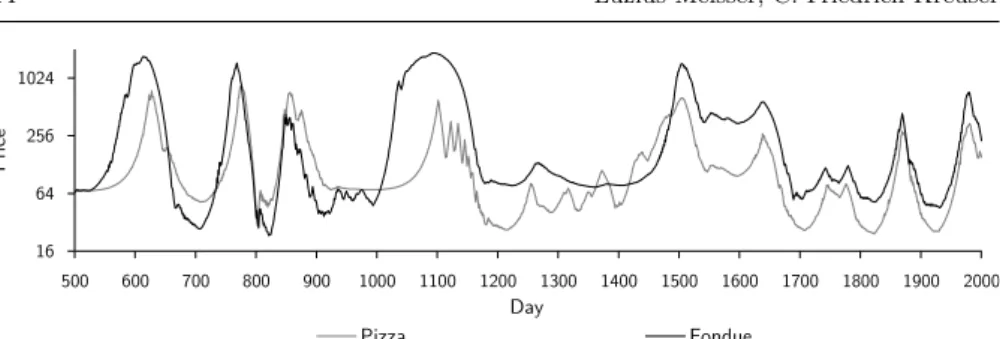
is the old fondue price and vice versa. Furthermore, as the Solper-Samuelson effect predicts, Italian and Swiss wages also switch. Figure 8 shows prices over time in the default configuration. It is accurate and stable, although there is a period of turmoil after the preference shock, during which production breaks down. Without production, there is not much to buy and thus no incentive to work either - contributing further to the decline of production. At the same time, consumer wallets are still refilled daily by dividend payments, leading to escalating prices until work pays off again, production recovers, and prices rebalance. Switching from exponential search to any of the other three ad-justment methods, accuracy is reduced and sporadic deviations start to occur endogenously, as shown in figure 9 with constant percentage adaption. Due to the random queueing of the consumers, there are constant small perturbations that can trigger endogenous price escalations. In contrast, exponential search is not as easily thrown off balance. As long as sensor pricing is enabled, the Stolper-Samuelson effect can be observed with all four adjustment strategies. Without sensor pricing, however, the system’s dynamics can turn as chaotic as shown in figure 10. Figure 11 finally shows how prices settle on unpredictable nominal levels when normalization is disabled.
16 64 256 1024 500 600 700 800 900 1000 1100 1200 1300 1400 1500 1600 1700 1800 1900 2000 Pr ic e Day Pizza Fondue
Fig. 10 Disabling sensor pricing in the default configuration can cause chaos.
2 4 8 16 32 64 500 1000 1500 2000 2500 3000 3500 4000 4500 5000 Pr ic e Day
Pizza Fondue Italian man-hour Swiss man-hour
Fig. 11 Without price normalization, nominal price-levels can change after shocks. The visible shocks are exogenously triggered by temporary preference changes. Without price normalization, firms equate dividends with profits instead of using the threshold heuristic form section 3.1.
4.3 Implementation
The simulation is written in Java and consists of about 100 classes with roughly 5000 lines of code. Its source code resides on stolsam.meissereconomics.com in a public git repository, a version control system recently recommended by Bruno (2015). Running CompEconCharts.java outputs CompEconCharts.out, which contains the raw data of all presented results. A single simulation run takes about one second, which is more than ten times faster than numerically solving the equivalent equilibrium model with the standard approach. We did not test faster ways of solving the equlibrium problem such as the method by Negishi (1972).
5 Conclusion
Replicating the Stolper-Samuelson effect in a simple setting with standard as-sumptions turned out to require more creativity than expected. Sensor pricing was introduced to address input synchronization, exponential search was ap-plied to increase accuracy, and dividend-based price normalization improved dynamics. The primary enabler for these innovations was having a rigorous quantiative benchmark, allowing to effectively and systematically test ideas. Replicating other easily verifiable phenomena could prove a fruitful path
for-wards for agent-based economics and greatly help establishing solid method-ological foundations for confidently building more complex models.
Acknowledgements We would like to thank Johannes Brumm and Gregor Reich for their valuable inputs, Abraham Bernstein for pointing us to system dynamics, Krzysztof Kuchcin-ski and Radoslaw Szymanek for the JaCoP solver, and participants of CEF 2015 – most notably Ulrich Wolffgang – for their helpful comments.
References
Arrow KJ, Debreu G (1954) Existence of an equilibrium for a competitive economy. Econometrica: Journal of the Econometric Society pp 265–290 Axtell R (2005) The complexity of exchange. The Economic Journal
115(504):F193–F210
Bentley JL, Yao ACC (1976) An almost optimal algorithm for unbounded searching. Information processing letters 5(3):82–87
Brock WA, Hommes C (1998) Heterogeneous beliefs and routes to chaos in a simple asset pricing model. Journal of Economic dynamics and Control 22(8):1235–1274
Bruno R (2015) Version control systems to facilitate research collaboration in economics. Computational Economics pp 1–7
Catalano M, Di Guilmi C (2015) Dynamic stochastic generalised aggregation in a multisectoral macroeconomic model. In: Proc. of the 21st Int. Conf. on Computing in Economics and Finance (CEF 2015)
Coase RH (1937) The nature of the firm. Economica 4(16):386–405
Deissenberg C, Van Der Hoog S, Dawid H (2008) Eurace: A massively paral-lel agent-based model of the european economy. Applied Mathematics and Computation 204(2):541–552
Eidson ED, Ehlen MA (2013) Nisac agent-based laboratory for economics (n-able): Overview of agent and simulation architectures
Elmaghraby W, Keskinocak P (2003) Dynamic pricing in the presence of in-ventory considerations: Research overview, current practices, and future di-rections. Management Science 49(10):1287–1309
Feldman AM (1973) Bilateral trading processes, pairwise optimality, and pareto optimality. The Review of Economic Studies pp 463–473
Gatti DD, Desiderio S, Gaffeo E, Cirillo P, Gallegati M (2011) Macroeconomics from the Bottom-up, vol 1. Springer Science & Business Media
Gintis H (2007) The dynamics of general equilibrium. The Economic Journal 117(523):1280–1309
Hommes C (2013) Behavioral rationality and heterogeneous expectations in complex economic systems. Cambridge University Press
Jones RW (1968) Variable returns to scale in general equilibrium theory. In-ternational Economic Review 9(3):261–272
Jones RW, Scheinkman JA (1977) The relevance of the two-sector production model in trade theory. The Journal of Political Economy pp 909–935
Kim DH (1992) Guidelines for drawing causal loop diagrams. The Systems Thinker 3(1):5–6
LeBaron B (2001) Empirical regularities from interacting long-and short-memory investors in an agent-based stock market. Evolutionary Compu-tation, IEEE Transactions on 5(5):442–455
Martin JP (1976) Variable factor supplies and the heckscher-ohlin-samuelson model. The Economic Journal 86(344):820–831
Milgrom P, Roberts J (1994) Economics, organization and management. Prentice-Hall
Negishi T (1972) General equilibrium theory and international trade
Riccetti L, Russo A, Gallegati M (2014) An agent based decentralized match-ing macroeconomic model. Journal of Economic Interaction and Coordina-tion pp 1–28
Rouchier J (2013) The interest of having loyal buyers in a perishable market. Computational Economics 41(2):151–170
Seppecher P (2012) A java agent-based macroeconomic laboratory
Stolper WF, Samuelson PA (1941) Protection and real wages. The Review of Economic Studies 9(1):58–73
Tesfatsion L (2006) Agent-based computational economics: A constructive ap-proach to economic theory. Handbook of computational economics 2:831– 880
Wolffgang U (2015) A multi-agent non-stochastic economic simulator. In: Proc. of the 21st Int. Conf. on Computing in Economics and Finance (CEF 2015)