Characterisation of Dynamic Process Systems by Use of Recurrence Texture Analysis

(1)

Western Australian School of Mines

Characterisation of Dynamic Process Systems by Use of

Recurrence Texture Analysis

Jason Bardinas

This thesis is presented for the Degree of Doctor of Philosophy

of

Curtin University

(2)

i

DECLARATION

To the best of my knowledge and belief, this thesis contains no material previously published by any other person except where due acknowledgment has been made.

This thesis contains no material which has been accepted for the award of any other degree or diploma in any university.

_________________________________________

Jason Bardinas

______________________________________ Date

(3)

ii

ABSTRACT

Many dynamic processes exhibit recurrent behaviour. This is an important feature that led to the idea that the recurrence of the states is a key element in the comprehensive understanding of dynamical systems. Although the recurrence has been known for a long time, its prevalence has just seen recently due to the advancement of computational technology especially in the visualisation of the recurrence of the states.

The recurrence plot is the most common method in studying the recurrence, which are often quantified by using Recurrence Quantification Analysis. Although proven effective, these methods only work when the distance matrix is compared to the threshold value, a significant parameter that can only be defined by the user. This threshold value actually dictate the features of the recurrence inside the plot. Although the so-called ‘unthresholded recurrence plot’ which is a mere distance matrix has already been proposed, its use is still limited due to the absence of reliable method that could extract useful features of the recurrence of the states from these plots. This research gap has been the motivation in the development of the proposed method which is termed as “Recurrence Texture Analysis”.

Recurrence Texture Analysis was stimulated in the hypothesis that the recurrence plots of dynamical systems, whether thresholded or not, are governed by a well-defined texture descriptors that can be extracted by some algorithms used for texture analysis. The validation of this premise and the evaluation of the method, along with the exploration of the use of deep neural networks and other texture extraction algorithms to quantify textures and hence the behaviour or dynamics of the time series data, were accomplished in this research. More specifically, the applicability of the method to capture the structures of complex dynamic process systems represented by time-series

(4)

iii

and characterise its dynamic behaviour were carried out systematically. These were done by transforming the recurrence patterns into sets of feature matrices containing the texture features. Conversely, the structures of time series are captured via the extraction of variables representing the distances between measurements over time. This is achieved through analysis of the structure of the data during discrete periods of process observation. These joint distributions of the elements in these distance matrices are subsequently captured by descriptors or features most often used in the analysis of textures from image data.

Six texture algorithms are considered in this research including the two state-of-the-art pretrained deep convolutional neural networks. The texture features extracted using grey-level co-occurrence matrix, wavelet transforms, local binary pattern, textons, CNN-AlexNet and CNN-VGG16 were analysed via cluster and classification analysis of the features. To verify the robustness of the method in dealing real process datasets, RTA was also applied in some datasets of grinding circuits and powder flow to characterise their dynamic behaviour. Furthermore, the method was also used as a data pre-processing technique in time-series classification task. The method was also extended as a core in the development of statistical process monitoring system.

Over the course of this research, RTA showed its applicability in capturing the textural features of recurrence that are relevant in the understanding of the dynamical behaviour of dynamic process systems. It has showed substantial advantage in the characterisation of the complex and dynamic properties of several processes over its counterparts. Specifically, the VGG16 provided that most discriminative textural features as demonstrated by its outstanding performance, outperforming other RTA methods and even to other published methods. Throughout this thesis, it consistently achieved highly competitive results against any other considered similar approaches. Furthermore,

(5)

iv

AlexNet and texton also displayed reliable performance in which they satisfactorily performed well over GLCM, wavelet and LBP and even to RQA. With this, it can also be said that these are also good candidates for capturing the structures of process systems.

It is also demonstrated in this thesis the applicability and effectiveness of pretrained CNNs (VGG16 and AlexNet) in capturing the dynamic behaviour of time series data eventhough the distance matrix plots are not included in the training stage of these algorithms. This further confirmed that these algorithms can be extended to other applications and used to other types of datasets. Most importantly, the thesis clearly showed the promising application and the pioneering work of recurrence texture analysis to minerals processing including grinding circuits, which would open more researches with the method and other related methods for minerals engineering application. In this work, it proved that the method could form the basis for more development of models for applications in minerals processing, which could in principle be used and implemented online once calibrated.

(6)

v

NOMENCLATURE

LIST OF ABBREVIATIONS AND ACRONYMS

2D two-dimensional

3D three-dimensional

AANN Autoassociative neural network ACF Autocorrelation function

AIC Akaike information criterion AMI Average Mutual Information ANN Artificial neural network AUC Area-under-the-curve

CF Cake Flour

CNN Convolutional neural network

CON Contrast

COR Correlation

CPV Cumulative Percent Variance CWT Continuous Wavelet Transforms

DPCA Dynamic Principal Component Analysis DWT Discrete Wavelet Transforms

EMI Eigenvalue-based Mutual Information

ENE Energy

ENTR Entropy

EOG Electrooculogram

FAR False alarm rate

FD Feed Disturbance

FL Feed Limited

FNN False Nearest Neighbour GAF Gramian Angular Field

(7)

vi

GADF Gramian Angular Difference Field GASF Gramian Angular Summation Field GLCM Grey Level Co-occurrence Matrix

GMM Gaussian Mixture Model

HOM Homogeneity

ILSCRC ImageNet Large-Scale Visual Recognition Challenge k-NN k-Nearest Neighbour

LBP Local Binary Pattern

LDA Linear Discriminant Analysis LM Leung-Malik filter bank LoG Laplacian of Gaussian

LOI Line of Interest

LTM Lagged Trajectory Matrix

LVPP Lotka-Volterra Predator-prey System MAE Mean-absolute-error

MAR Missing Alarm Rate

Max Maximum

MF Maize Flour

Min Minimum

MISSQ Minimal Increase of Sum-of-squares MRP Multi-level Recurrence Plot

MSE Mean-square-error

MTF Markov Transition Field

NLPCA Nonlinear Principal Component Analysis NOC Normal Operating Condition

PC Portland Cement

PCA Principal Component Analysis PLS Partial Least Squares

(8)

vii

Q Quartz

R2 _{Coefficient of Determination}

RF Random Forest

RFS Root Filter Set RI Rotation Invariant

RL Run Length

RMSE Root-mean-square-error

ROC Receiving Operating Characteristics

RP Recurrence Plot

RPCD Recurrence Patterns Compression Distance RQA Recurrence Quantification Analysis

RR Recurrence Rate

RTA Recurrence Texture Analysis

SFTA Segmentation-based Fractal Texture Analysis SOM Self-organising Maps

SSA Singular Spectrum Analysis SVD Singular Value Decomposition SVM Support Vector Machine

TE Tennessee Eastman Problem

TFRP Texture features from Recurrence Patterns

TS Table Salt

UTRP Unthresholded Recurrence Plot

LIST OF SYMBOLS

a, b, c Scaled time ratios of the autocatalytic reaction

b Window width

B Bias term

(9)

viii

c Convolutional output (subscript: H for horizontal, A for approximation, D for diagonal, and V for vertical)

c Number of dimensions (column) in time series Y 𝐶_𝑐 _{Cophenetic correlation function}

𝐶̂ Reaction rate or the frequency of the contact of the prey and predator

Cp Controlling parameter

d Distance

D Distance matrix

𝐷̂ Conversion efficiency or the efficiency of predators in converting food into offspring

db4 Daubechies wavelet family

𝐸 _{Error in Sammon map}

𝑬 _{Residual matrix}

F Number of features

f Lower dimensional latent variable in LDA

𝐹₀(𝑡̇, 𝜎) _{Zero direct current component guarantor}

g Image pixel (subscript: c for center, p for neighbouring pixel)

G Number of grey level

h Histogram bin

I Image

𝐼𝐺 Greyscale image

𝐼_𝑠𝑐 _{Greyscale image (scaled)}

J All-ones matrix

K Predator-prey rate (subscript: 1 for prey population growth, 2 for predator mortality)

(10)

ix

K (xi, xj) Kernel function L Diagonal line length L Segmented time series

L Primal Lagrangian

L2- norm Euclidean norm

L∞-norm Maximum or Supremum norm

m Sliding step

md Embedding dimension

n Number of observations

N Number of segments (distance matrix) Nn Average number of neighbours

Np Number of significant peaks in density plot

𝑷 _{Loading matrix}

p(•) Probability function

p(•,•) Joint probability function

𝑝(𝑥|𝜃𝑖) Probability density function

𝑝̂_𝑖,𝑗 _{Pixel pair entry in (i,j)}

𝑝̂(𝒛|𝜔𝑘) Conditional density of the number of samples Nk

within the class 𝜔𝑘 Q-res Q-residuals

r Number of classes

R Recurrence matrix

𝑅(𝒛) _{Hypersphere with volume V(z) with z as the center of} R(z)

𝑹_𝑖,𝑗 (𝑢𝑛𝑡ℎ𝑟𝑒𝑠) _{Unthresholded recurrence plot} s Scale parameter of the signal s LBP operator threshold value Ѕ Schmid Filter Set

(11)

x

T Texton channel

𝑻 _{Score matrix in PCA}

𝑇_𝑐 _{Transitivity coefficient} Tn Recurrence time T2 _{Hotelling’s T-squared}

𝑡̇ _{Cycle count in the harmonic function} u Discrete time series

U Uniformity measure

𝑢̅ _{Mean of time series}

V Vertical line

W Transformed function

𝑤 _{Scaling filter (subscript: H for high, L for low)}

𝒘̇ _{LDA transformation}

x, y, z Feed concentration variables involved in autocatalytic reaction

X Feature matrix or data matrix

𝑥̇ _{Number of prey}

𝑥⃑ _{Trajectory point}

Y Parent time series

𝑦̇ _{Number of predator}

𝛾 _{Scaled feed concentration ratios}

𝝈 _{Gaussian noise}

𝜎2

Standard deviation

𝜺 _{Threshold distance or neighbourhood size} θ Angle of grey levels

𝚯 _{Heaveside function}

𝜆 _Eigenvalues

(12)

xi

𝜏 _{Translation parameter}

𝜉𝑖 Slack variable in SVM

𝜓 _Wavelet

ψ (•) Pre-defined function mapping

(13)

xii

ACKNOWLEDGMENTS

My PhD journey is indeed a roller-coaster ride with many ups and downs. But as a wise man once said, “There is always light at the end of the tunnel”. Of course, the journey towards this tunnel is made up of several challenges in many forms, but these challenges have transcended into triumphs because of the people mentioned here who supported me along the way.

First of all, I would like to express my deepest gratitude to my supervisors, Prof. Chris Aldrich and Dr. Boris Albijanic, for their guidance throughout this journey. I have learned more about the world of data, and the world in general, from them in the past three years of my life than I would ever have imagined was possible. Special mention to Chris for his patience he has given on me during the times when the light of the tunnel is nowhere to be found.

I extend many thanks to WASM and to Curtin International Postgraduate Research Scholarship (CIPRS) for the financial support and scholarships. Without this grant, this PhD journey would most likely not become possible.

I would also like to mention the support of my friends who have supported me during the periods where I felt so down and empty. Special shout out to France for the help and support especially in producing this manuscript.

Most especially, I would like to give my deepest gratitude to my family, particularly to my loving parents. Thank you for their encouraging words of wisdom and for always believing in me despite everything I have been through. Ultimately, I would like to thank the Almighty God in heaven. Thank you for the gifts of life and the power of believing in my works and in myself in general. I could never have this PhD without the faith I have in You.

(14)

xiii

PUBLICATIONS

This thesis includes the following works that have been submitted for publication over the course of my PhD study:

Bardinas, J., Aldrich, C., & Albijanic, B. (2016). Identification of the dynamic behaviour of an autogenous mill by use of time series cluster analysis.

Proceedings of the XXVIII International Mineral Processing Congress (IMPC 2016).

ISBN: 978-1-926872-29-2, September 11 – 15, 2016, Québec City, Canadian Institute of Mining, Metallurgy and Petroleum. [Chapter 7]

Bardinas, J., Aldrich, C., & Napier, L. (2018). Predicting the operating states of grinding circuits by use of recurrence texture analysis of time series data.

(15)

xiv

LIST OF FIGURES

Figure 2-1. Three norms for the neighbourhood with same radius: L1-norm (A),

L2-norm (B), L∞-norm (C). ... 9

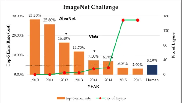
Figure 2-2. Sample RPs showing different typology: (A) homogeneous (uniformly distributed noise), (B) periodic (super-positioned harmonic oscillations), (C) drift (logistic map corrupted with a linearly increasing term), and (D) disrupted (Brownian motion). ... 14 Figure 3-1. Schematic workflow of the study, comprising the time series data (A), segmentation of the data (B), calculation of distance matrix for each time series segment (C), and extraction of texture features from each matrix (D). 26 Figure 3-2. Samples of the distance matrices showing the different structures for different classes ... 30 Figure 3-3. Illustration showing the GLCM calculation ... 40 Figure 3-4. Discrete two-dimensional wavelet decomposition at level j. cA, cH, cV and cD refer to approximation and detail coefficients. wL and wH refer to the high pass and low pass filters, respectively. The circles containing “2” and a downward arrow indicate down sampling of the coefficients by retaining only every other row or column. ... 46 Figure 3-5. Local binary pattern operations, showing (a) the intensity values of the centre pixel (shaded) and its neighbours in the original image, (b) the corresponding thresholded values, and (c) the neighbouring pixel values converted to powers of 2 according to location and summed for the centre pixel. ... 48 Figure 3-6. Learning steps involved in extracting texton features ... 51 Figure 3-7. Historical performance of ImageNet Challenge from 2010 to 2016 showing both the error rate and the number of layers of the networks. ... 55 Figure 3-8. Typical CNN architecture ... 55 Figure 3-9. The architecture of AlexNet... 59

(21)

xx

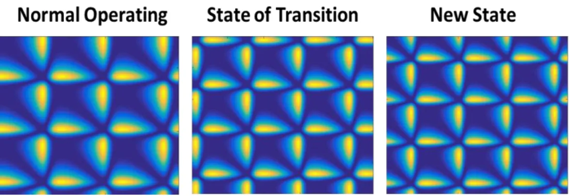
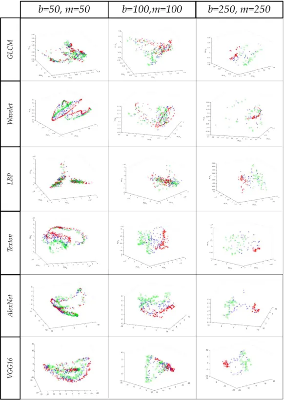
Figure 3-10. The simplified diagrams showing the architectures of AlexNet (top) and VGG16 (bottom). It highlights the similarity and differences in terms of the structures of convolutional (Conv), pooling (Pool), and fully-connected (FC) layers. ... 60 Figure 4-1. Simulated observations of the Lotka-Volterra predator-prey model. ... 65 Figure 4-2. Autocorrelation function of Lotka-Volterra Predator-prey system ... 66 Figure 4-3. Distance matrix plots of three states of the system using Euclidean distance. Top and bottom plots show the 10,000-by-10,000 and 100-by-100 matrix plots of the time series, respectively. ... 67 Figure 4-4. RTA feature sets projected in 3-D principal component subspace, using different values of window width b: b=50 (left), b=100 (middle), and b=250 (right). The distance matrix is constructed using Euclidean distance with fixed sliding step m=50. The legends red (*), blue (+) and green (o) correspond to NOC, state of transition, and new state, respectively. ... 68 Figure 4-5. RTA feature sets projected in 3-D principal component subspace, using fixed windowing. The distance matrix is constructed using Euclidean distance with three different window widths, b=50, 100 and 250. Legends are : red (*), blue (+) and green (o) correspond to NOC, state of transition, and new state, respectively. ... 71 Figure 4-6. Distance matrix plots of three states of the system using Chebychev distance or Maximum Norm. Top and bottom plots show the 10,000-by-10,000 and 100-by-100 matrix plots of the time series, respectively. ... 75 Figure 4-7. Visualisation of the RTA feature sets using the Euclidean distance (left) and the Chebychev distance (right) as projected into 3-D subspace using the first 3 principal component scores. Legends are : red (*), blue (+) and green (o) correspond to NOC, state of transition, and new state, respectively. ... 77

(22)

xxi

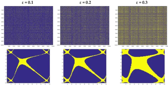
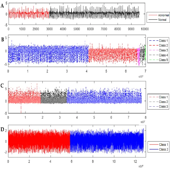
Figure 4-8. Recurrence plots having different ε: ε=0.1 (left), ε=0.2 (middle), ε=0.5 (right), using Euclidean norm. Top and bottom plots correspond to 10,000-by-10,000 and 100-by-100 matrix recurrence plots. ... 79 Figure 4-9. Visualisation of the RQA feature sets with different ε values using the Euclidean distance (left) and the Chebychev distance (right) as projected into 3-D subspace using the first 3 principal component scores. The time series is segmented using b=100 and m=50. Legends are: red (*), blue (+) and green (o) correspond to NOC, state of transition, and new state, respectively. ... 81 Figure 4-10. Texton features as projected into 3-D nonlinear principal component subspace using (A) Euclidean distance, and (B) Chebychev distance. Legends are : red (*), blue (+) and green (o) correspond to NOC, state of transition, and new state, respectively. ... 82 Figure 4-11. RP plots of three state systems of Lotka-Volterra predator prey system. Constructed using Euclidean norm, ε = 0.2. ... 82 Figure 4-12. 3-D plots of different feature sets obtained from recurrence plots: GLCM (A), wavelet (B), LBP (C), textons (D), Alexnet (E), VGG16 (F) and RQA (G). The plots are constructed in 3-D using the first three principal component scores. Legends are : red (*), blue (+) and green (o) correspond to NOC, state of transition, and new state, respectively. ... 84 Figure 5-1. Plots of the training datasets of (A) ECG200, (B) ECG5000, (C) Chlorine Concentration, and (D) Yoga time series. The plots are also colour-coded that correspond to the classes. ... 89 Figure 5-2. The Autocatalytic process time-series data ... 91 Figure 5-3. Representative samples of distance matrix plots of the training datasets of four UCR Time Series Archive used in the study ... 97 Figure 5-4. Exemplary distance matrix plots of the autocatalytic process system showing NOC (left), transition (middle) and new state system (right) ... 100

(23)

xxii

Figure 5-5. RTA-Texton (left) and CNN-VGG16 (right) features showing maximum separability between states in linear discriminant subspace ... 102 Figure 6-1. Basic diagram of a fully-autogenous mill ... 108 Figure 6-2. The normalised time-series mill load with labelled states: (I) NOC, (II) Feed disturbance, (III) Feed limited ... 108 Figure 6-3. The Autocorrelation Function (ACF) of the mill load time series showing b=250. ... 109 Figure 6-4. Representative plot of the Euclidean distance matrices of three operational states of the autogenous mill ... 110 Figure 6-5. Visualisation of the texton-schmid feature sets of mill load data as projected onto 2D space using the linear discriminant scores. ... 111 Figure 6-6. Flow diagram of the IsaMill grinding circuit, showing the measuring points of the power, temperature, and P80 particle sizes ... 113 Figure 6-7. The raw time-series of power draw (top) and temperature (middle) of the autogenous mill, and the corresponding particle size measurements (bottom) ... 115 Figure 6-8. The outlet temperature versus power draw plot with corresponding colour legends on the particle size classes. ... 116 Figure 6-9. The distribution of particle sizes showing the partitions of 3 classes (fine, intermediate, and coarse) ... 116 Figure 6-10. The autocorrelation function (left) and false nearest neighbour plots (right) of power draw and outlet temperature time series ... 117 Figure 6-11. Distribution of training (black ‘o’) and test (red ‘∗’) data sets. . 118 Figure 6-12. Distance matrix plots of 3 classes: fine (left), intermediate (middle) and coarse (right) using time series of power draw (top), outlet temperature (middle) and cross distance of these variables (bottom) ... 120 Figure 6-13. The reconstructed attractors of power draw (left) and outlet temperature (right) time series data with legend: fine (red ‘∗’), intermediate (blue ‘+’), and coarse (green ‘o’). ... 124

(24)

xxiii

Figure 6-14. Linear projection of combined power draw and temperature texton (I), AlexNet (II) and VGG16 (III) features showing maximum separability between classes: fine (red ‘*’), intermediate (blue ‘+’) and coarse (green 'o') ... 124 Figure 6-15. Schematic diagram of the experimental setup showing the a vessel (A) powders flow through an orifice (B) onto a base plate (C) and overflow is measured in digital balance (D) connected to computer (E) ... 127 Figure 6-16. The raw time-series mass data of the five powders ... 128 Figure 6-17. The autocorrelation function of the powder time series data, showing b=1000. ... 128 Figure 6-18. Euclidean distance matrices (with colour maps) of the Portland cement (A), Cake flour (B), Maize flour (C), Quartz (D), and Table salt (E) 129 Figure 6-19. Textural features of (A) GLCM and wavelet, (B) LBP, (C) texton, and (D) combined GLCM, wavelet, LBP and texton, (E) AlexNet, and (F) VGG16 as projected onto 3-D principal component subspace ... 130 Figure 6-20. Linear discriminant projection of RTA features namely (A) GLCM and wavelet, (B) LBP, (C) textons, and (D) all features (GLCM, wavelet, LBP, textons), showing maximum separability between the powders. ... 132 Figure 6-21. Exemplary samples of recurrence plots of (A) Portland cement, (B) cake flour, (C) maize flour, (D) quartz, and (E) table salt. ... 134 Figure 6-22. 3-D plot of the RQA features using the first 3 principal component scores. ... 135 Figure 7-1. Extraction of features from time series data (A), by segmentation into nonoverlapping segments (B), derivation of Euclidean matrices for all the segments (C) and extraction of features from these distance matrices (D). These features or variables can subsequently be used to build models (E) and to derive diagnostics (F) for process monitoring. ... 140 Figure 7-2. General flowchart showing the online application of the dynamic process monitoring model ... 144

(25)

xxiv

Figure 7-3. Simulated observations of the Lotka-Volterra predator-prey model. ... 146 Figure 7-4. Exemplary plots of distance matrices of the three conditional states of the Lotka-Volterra predator-prey model ... 148 Figure 7-5. Plots of the first two principal components scores of the extracted features (CPV=66.68%) along with the trained 1-class GMM decision boundary (K=2), and its decision criterion plot... 149 Figure 7-6. The Hotelling’s T2_{(top) and Q-res (bottom) plots of extracted}

features. ... 150 Figure 7-7. The Hotelling’s T2_{(top) and Q-index plot (bottom) of extracted}

features with a window width of b = 100. ... 156 Figure 7-8. Representative plots of distance matrices (80-by-80 matrix) of the NOC and faults datasets of TE problem ... 161

(26)

xxv

LIST OF TABLES

Table 2-1. Visual Interpretation of recurrence plots ... 15 Table 2-2. The RQA features, and its corresponding descriptions ... 16 Table 3-1. Hyperparameters of the texture extraction algorithms used in the study ... 31 Table 4-1. Summary of the parameters used in three condition states (NOC, state of transition and new state) ... 66 Table 4-2. Influence of windowing parameters to the overall classification performance of RTA features (classification accuracy on the test data) ... 73 Table 4-3. Parameters used in the study on the influence of distance metric to the overall performance of RTA ... 74 Table 4-4. Comparison of the classification performance of the RTA and RQA feature sets using Euclidean and Chebychev distance metrics. The reported classification accuracy is based on the test datasets. ... 75 Table 4-5. Classification performance of RTA features applied to recurrence plots ... 83 Table 5-1. Summary of the four UCR time series datasets used in this case study ... 89 Table 5-2. Hyperparameters of the texture extraction algorithms used in the study ... 94 Table 5-3. Results of the classification performance of RTA during the training and testing stages ... 98 Table 5-4. Comparison of the error rates of the proposed method (RTA) to other approaches (TFRP and RPCD) ... 99 Table 5-5. Results of the classification accuracy on the test dataset of autocatalytic process ... 101 Table 6-1. Mill load time-series data ... 109 Table 6-2. Power Draw and Outlet Temperature data ... 117

(27)

xxvi

Table 6-3. Results of classification (% correct) with predictor sets derived from the mill power data and use of a cubic kernel support vector machine. ... 121 Table 6-4. Results of classification (% correct) with predictor sets derived from the mill temperature data and use of a cubic kernel support vector machine. ... 122 Table 6-5. Results of classification (% correct) with predictor sets derived from the cross recurrence combination of mill temperature and power data and use of a cubic kernel support vector machine. ... 122 Table 6-6. Results of classification (% correct) with predictor sets derived from combination of the mill temperature and power data and use of a cubic kernel support vector machine. ... 123 Table 6-7. Mass data of the powders ... 127 Table 6-8. Classification performance of the feature sets (highlighted the highest classification accuracy in the test dataset) ... 133 Table 7-1. Hyperparameters used in GLCM and wavelet feature extraction. ... 141 Table 7-2. Parameter variations used in three condition states (NOC, transition and new). ... 147 Table 7-3. Summary of data and model parameters used in the LVPP ... 147 Table 7-4. Setting parameters used in Random forest model ... 152 Table 7-5. Setting parameters used in circular inverse NLPCA ... 153 Table 7-6. Summary of the performance metrics of the two fault detection methods on the Lotka-Volterra predator-prey model time series. ... 155 Table 7-7. Description of variables in Tennessee Eastman process. ... 158 Table 7-8. Description of faults in the Tennessee Eastman process. ... 159 Table 7-9. Summary of data and model parameters used in the Tennessee Eastman (TE) process case study. ... 160

(28)

xxvii

Table 7-10. Results of the performance of the process monitoring method to the faults of TE process using the Hotelling’s T2_{, Q-residuals, and GMM}

(29)

1

1. INTRODUCTION

1.1 Complexity in Dynamical Systems

Many natural and man-made systems show complex and nonlinear behaviour. In process engineering, this includes grinding circuits (Aldrich, Burchell, de V. Groenewald, & Yzelle, 2014), fluidized beds (Johnsson, Zijerveld, Schouten, van Den Bleek, & Leckner, 2000; Llop, Gascons, & Llauró, 2015; Pain, Mansoorzadeh, Gomes, & de Oliveira, 2002), multiphase flow (Keska, Smith, & Williams, 1999), multistage evaporation of liquor in the Bayer process used for alumina production by Alcoa (Kam, 2000) etc. – a cultivating idea that encouraged the emergence of the concept of complex systems, an area that is concerned with the understanding of the complexity and properties of the systems. Atay (2010) describes this subject as a study of any process or system that is comprised of numerous parts that produce macroscopic behaviour with a manifestation of forming distinctive temporal, spatial or functional structures.

While complex systems can be considered through different metaphors, such as bio-inspired algorithms (Cotta & Schaefer, 2017), cellular automata (Kotyrba, Volna, & Bujok, 2015), complex network theory (Mei, Zarrabi, Lees, & Sloot, 2015), chaos theory (e.g. (Sivakumar, 2004)) and others, the nonlinear time series analysis theory developed over the last four decades (e.g. (Kantz, 2004; Sprott, 2003)) is arguably one of the most important.

1.2 Phase Space Approach to Time Series Analysis

The basic point of departure in nonlinear time series analysis is that it contains repetitive patterns that can be analysed in a so-called phase space, which is simply a projection of the observed time series data onto a new

(30)

2

coordinate system consisting of number of lagged time series variables. That is,

𝑦(𝑡) → [𝑥(𝑡), 𝑥(𝑡 − 𝑘), … 𝑥(𝑡 − (𝑚 − 1)𝑘)] (1-1)

Two parameters define the projection, namely the time series lag, 𝑘 and the embedding dimension, m of the time series. Most of the time, the time series lag k is estimated by either the use of autocorrelation function of the average mutual information (Jemwa, 2003). The embedding dimension, m, on the other hand, can be assessed by several methods including singular value decomposition, and false nearest neighbours.

The repetition of patterns in the time series data are often referred to as “recurrence”, which is considered a fundamental property in many dynamical systems. The recurrence is commonly visualised using recurrence plots, which are derived from a phase space embedding of the time series data, which are constructed based on distance matrix. Although embedding of the time series data is commonly done prior to construction of recurrence plots, this is not strictly necessary, as was shown by Iwanski and Bradley (1998) and March, Chapman, and Dendy (2005). In general, the recurrence point observed in the plot is a distance matrix element having a distance less than or equal to a specified neighbourhood size or threshold value, 𝜀. This plot generally gives recurrence patterns, which are normally quantified using recurrence quantification analysis (RQA).

Although RQA is a highly versatile tool and has seen considerable success in various applications, (Hou, Aldrich, Lepkova, Machuca, & Kinsella, 2016; Souza, Silva, & Batista, 2014; Webber Jr, Marwan, Facchini, & Giuliani, 2009), it suffers from two drawbacks when used as a means to generate features of predictors for generalized time series analysis. First, thresholding

(31)

3

the plot results in a loss of information, which may be important in subsequent analysis. Second, powerful as they are, RQA features are essentially hand crafted and may not be the optimal features required for a given analysis.

One of the logical thoughts in addressing these limitations in RQA is to eliminate the incorporation of the threshold value in constructing recurrence plots. Although the use of so-called “unthresholded recurrence plots (UTRP)” has recently been proposed (Sipers, Borm, & Peeters, 2011, 2017), the utilisation and full implementation is limited as yet, as there is still no well-established quantification method that can be employed to describe the features of the recurrences contained within these plots In fact, some researchers like Acuña-González, García-Ochoa, and González-Sánchez (2008) for example, mention the lack of analytical means explicitly as a reason for not using unthresholded recurrence plots. This challenge has motivated the development of the proposed method in this thesis.

1.3 Recurrence Texture Analysis: A Novel Method in

Characterising the Recurrence

One could say the UTRP is basically just a distance matrix since each element is not compared to a threshold value nor transformed into binary form. In fact, the idea of UTRP has been known for quite some time, especially in the context of nonlinear data analysis.

UTRP or distance matrix plots commonly provide noticeable elements even to the small variations in the distances between the recurrence points (Savari et al., 2017) that sometimes are not reflected in the thresholded recurrence plots. While this becomes a significant advantage of UTRP, this is not commonly exploited, mainly due to its difficulty in quantifying the recurrence features contained in the plot. There is at present no established

(32)

4

method that can be employed to extract useful features in UTRPs, since RQA is only applicable to thresholded RPs.

A basic idea that motivated the development of this thesis is that the recurrence plot, whether thresholded or not, can also be viewed as a texture, the nature of which is determined by the recurrence or repetition of patterns in the time series data. This means that a time series, as represented by a distance matrix, can be characterised by examining the texture of recurrences. For it to make sense, these textures could be extracted for further analysis, which could be possible through the use of several texture modelling techniques.

Texture modelling, as commonly used in image analysis and computer vision, is considered a novel approach on studying dynamic systems. Literature reviews suggested that the incorporation of texture in analysing the distance matrix of the time series, and hence of the structure of dynamical systems is not well established yet.

Moreover, the encoding of time series into images allows one to take advantage of recent developments in state-of-the-art algorithms in image analysis. This includes, in particular, the deep convolutional neural networks that are currently enjoying massive interest among researchers and developers, owing to their proven ability to quantify discriminative textures are also considered an innovative approach for time series analysis.

The use of recurrence texture analysis explored in this thesis therefore aims to take advantage of the fact that the behaviour of time series data can be expressed as textures in distance matrices derived from these data. In tandem with this, it also aims to explore the use of deep neural networks to quantify these textures and hence the behaviour or dynamics of the time series data.

(33)

5

1.4 Objectives

The general aim of this study is to evaluate the applicability of the recurrence texture analysis in characterising dynamic process systems and subsequent analysis of their dynamic behaviour.

This main objective will be achieved by the accomplishment of the following tasks:

 The analysis of the method and its performance in analysing time series by:

o extraction of texture features of distance matrix plots using several textural extraction algorithms, including those based on the use of pretrained deep convolutional neural networks

o evaluation of the influence of parameters of the methodology, specifically the window length and type of distance metric used on the overall performance of the method. o comparison of results to other approaches, particularly the use of RQA features, from which this approach is derived.

 The application of the method in dealing with time series analysis typically associated with applications in the process industries, namely:

o time series classification of benchmark data sets

o application of the proposed method to real datasets such as in grinding circuits and solids processing time series data

 Assessment of the performance of dynamic process monitoring systems derived from the method, via:

o application of the method on simulated data and a benchmark process engineering dataset

(34)

6

o comparison of the results to other related approaches.

1.5 Scope

The thesis, as a whole, is a proof-of-concept study of the proposed method, which is mostly concentrated on the evaluation of the method as a viable tool in analysing the structures of dynamical systems. In particular, although other benchmark datasets are used, the thesis is comprehensively focused on the evaluation of the method to dynamic process systems.

This thesis involves applying the method to time series classification employing RTA as data preprocessing method, and dynamic process monitoring or fault detection, using actual data sets, simulated and benchmarked datasets and public data sets. The thesis primarily focuses on applications to minerals engineering time series and consequently on the understanding of the nonlinear and dynamic behaviour of minerals processing datasets, such as in grinding circuit. In terms of texture modelling, the algorithms used to extract textures are limited to texture classification algorithms, hence, this specifically excludes spectral feature extraction and regression.

Ultimately, this thesis does not constitute an end-product that is all set for application in a real scheme. Rather, this work contributes towards the long-term goal of developing more effective methods that deal with nonlinear and dynamic behaviour of systems.

1.6 Outline of Thesis

This thesis is organised as follows: In Chapter 2, literature review on the unthresholded and thresholded recurrence plots and the time series analysis based on these plots are presented. Following this, in Chapter 3, the analytical

(35)

7

methodology is formalised and explained, including the general approach and the texture analytical algorithms considered in the investigation. Subsequent chapters deal with the application of the methodology, i.e. Chapter 4 details the results of the preliminary study of the method using simulated time series. The influence of parameters involved in employing the proposed method are studied in this chapter and the results are compared to RQA. In Chapter 5, the method is applied to time series classification on publicly available and simulated time series data sets. In Chapter 6, the dynamic behaviour of powder flow and autogenous mills are characterised using the method. In Chapter 7, the method is used as a framework for dynamic process monitoring based on the use of principal component models. Finally, Chapter 8 closes with the most important conclusions and recommendations from the study.

(36)

8

2. RECURRENCE IN DYNAMICAL SYSTEMS

2.1 Recurrence Plots

The recurrence plot (RP) is a graphical representation of recurrent patterns in a time series. First introduced by Eckmann (1987), the RP can visually describe the recurrence characteristic of many dynamical systems. It is a two-dimensional squared binary matrix wherein both axes represent time which is based on the distance measured. Formally, the recurrence matrix R of state 𝑥⃑ can be obtained using two time i and j along a phase space trajectory such that:

𝑹_𝒊,𝒋 = 𝚯(𝜺 − ‖𝒙⃑⃑⃑_𝒊 − 𝒙⃑⃑⃑_𝒋 ‖) , i , j = 1, 2, 3, … N (2-1)

where N is number of states under consideration, 𝜺 is the threshold distance, ‖ ∙ ‖ is the norm in the phase space and 𝚯 is the Heaviside step function (Marwan, Kurths, & Foerster, 2015; Schultz, Spiegel, Marwan, & Albayrak, 2015). Since the recurrence matrix R is a binarised matrix, the RP is then plot using two different colours (i.e. black and white). That is, at coordinates (i,j), if 𝑹𝒊,𝒋 = 1, a black dot is drawn as opposed to a white dot if 𝑹_𝒊,𝒋 = 0. Further, the RP always contains a black main diagonal line that correspond to 𝑹𝑖,𝑗 = 1|𝑖=1𝑁 . The diagonal line is commonly referred to as the line of identity (LOI). It is important to note that RP generally exhibits symmetry with respect to LOI ( 𝑹𝑖,𝑗 = 𝑹𝑗,𝑖). In some cases, although it is not required, a phase space reconstruction is carried out in constructing RPs, which requires embedding the data to other phase space using embedding parameters (e.g. time lag, embedding dimension).

Based on eqn (2-1) , RP is dependent on the type of norm ‖ ∙ ‖ and threshold distance 𝜺. These factors and parameters should always be taken

(37)

9

into account when generating RP. In the next subsections, the emphasis on the effect of these parameters are discussed in detail.

2.1.1 The Choice of Norm

From a theoretical point of view of RPs, the choice of norm is deemed to be insignificant. However, it is not the case when it comes to practical purposes as the visual characteristic of RPs could change for different norms (Bradley & Mantilla, 2002). This is attributed to the fact that the choice of norm (‖ ∙ ‖) dictates its structure brought about by the different shapes of neighbourhood.

Figure 2-1. Three norms for the neighbourhood with same radius: L1-norm (A), L2

-norm (B), L∞--norm (C).

In the comprehensive review of RP made by Marwan, Carmen, Thiel, and Kurths (2007), three commonly used norms are considered. These are the L1- norm, L2- norm (more commonly known as Euclidean norm) and the L∞-norm (also known as the Maximum or Supremum L∞-norm). As an example, for fixed ε, these norms generate different shapes of neighbourhood. The L∞-norm gave the most number of neighbours, followed by the Euclidean L∞-norm (L2- norm), and then L1-norm. With this outcome, it is emphasised that L∞-norm is the best option in constructing RP, mostly because of its computational efficiency. At some point, the Euclidean norm was also seen as a good norm in many studies involving RPs (Hou et al., 2016; Javorka, Turianikova,

(38)

10

Tonhajzerova, Javorka, & Baumert, 2009; Zbilut, Zaldivar-Comenges, & Strozzi, 2002).

2.1.2 The Choice of Threshold Distance

The neighbourhood size, more commonly known as the threshold distance, 𝜺 is another parameter of consideration when constructing RPs. A good value of 𝜺 has the capability of retaining more unique dynamically useful information while minimising the redundant information that could trigger misinterpretation of the features of recurrence (Schultz, Zou, Marwan, & Turvey, 2011). Normally, this is a user pre-defined parameter.

The structures of RPs generally depend on how large or small the chosen 𝜺 is. For instance, if 𝜺 is too small, recurrence structure becomes futile since no recurrence points are observed. On the contrary, 𝜺 being too large would result to a lot of artefacts and noise since the space considered is unreasonably vase such that every point is considered a neighbour of every other points (Marwan et al., 2007). With this, careful consideration is of utmost importance in identifying the optimal value of 𝜺.

A number of researchers have dedicated their efforts to studying this parameter and some of them established several “rules of thumb” in selecting 𝜺. For most studies, the 𝜺 is selected based on known information obtained from RP and phase space. This can be grouped into three: use of phase space diameter, use of the standard deviation of the noise present, and use of RP structures (i.e. recurrence point density, diagonal line).

For instance, in the work of Mindlin and Gilmore (1992), they used an estimate of 𝜺 by determining a few percent of the diameter of the attractor using its minimum and maximum value ( 𝜺 ~ 𝟏𝟎−𝟐𝒙 {𝒎𝒂𝒙[𝒙(𝒊)] − 𝒎𝒊𝒏[𝒙{𝒊)]}). Similarly, Zbilut and Webber (1992) used a small value of 𝜺

(39)

11

relative to the noise level. In addition, they noted that the value is generally not be greater than 10% of the normalised mean phase space diameter. In the work of Schinkel, Dimigen, and Marwan (2008), they inferred that, in the context of signal classification and discrimination, the most acceptable threshold value 𝜺 is about 5% of the maximum phase space diameter.

In the study of Thiel et al. (2002) on the effect of observational noise on the RPs, they found out that noise could significantly change the features and properties of RPs, thus observational noise should be taken into account when constructing RPs, particularly in threshold value. They proposed that 𝜺 should be at least five times the standard deviation of the observational Gaussian noise, σ (𝜺 > 𝟓𝝈).

The 𝜺 can also be estimated using features obtained in RPs. For instance, the use of recurrence point density could approximate the value of 𝜺. A good value of 𝜺 is obtained if the recurrence point density is about 1% (Zbilut et al., 2002). For (quasi-)periodic processes, the information on the diagonal structures of RP can also be used to estimate 𝜺. (Marwan et al., 2007) claimed that a good valueis 𝜺 is one that could minimize the quantity 𝛽(𝜀).

𝛽(𝜀) =|𝑁𝑛(𝜀) − 𝑁𝑝(𝜀)| 𝑁𝑛(𝜀)

(2-2)

where Np is the number of significant peaks in a certain density plots, Nn is the

average number of neighbours. In other words, 𝜺 is said to be optimised when Np is maximised and Nn approaches Np. While this estimation works well

especially for de-noising applications, the significant distribution of the diagonal lines in RP could be compromised if observational noise is present in the signal. To address this, the use of fixed recurrence point density and the use of fixed number of neighbours for every point were proposed. With the

(40)

12

fixed recurrence point density, more information is preserved, which allows for comparison of RPs even without undertaking time series normalisation prior to analysis.

Overall, even though there are already methods and guidelines available in determining 𝜺, there is still no strict rule that governs in determining optimal 𝜺. It is still largely dependent on the user/s and the type of systems being considered. In this sense, 𝜺 is a drawback in RPs, and therefore eliminating the use of this value is a good topic to research on as it has not been widely explored yet.

2.2 Unthresholded Recurrence Plots

The so-called “unthresholded RPs” is one of the variations of RPs. Generally speaking, it is referred to the distance plot since these RPs does not require any threshold distances and did not undergo binarisation (using Heaviside function) (Iwanski & Bradley, 1998). To some, it is also referred to as global recurrence plots (Webber Jr & Zbilut, 2003). Formally, the unthresholded RPs 𝑹𝑖,𝑗 (𝑢𝑛𝑡ℎ𝑟𝑒𝑠) is determined using eqn (2-3), which is identical to the equation used in calculating distance matrix.

𝑹𝑖,𝑗(𝑢𝑛𝑡ℎ𝑟𝑒𝑠) = ‖𝒙⃑⃑⃑𝒊 − 𝒙⃑⃑⃑𝒋 ‖ 𝑓𝑜𝑟 𝑖 = 1, 2, 3 … 𝑁 (2-3)

where ‖ ∙ ‖ is the norm in the phase space.

Some researchers have directed their attention to the examination of the unthresholded RPs on the basis of possessing and providing as much information and explanation on the mechanism of the considered dynamic system (or signal) in diverse areas, including the interpretation of financial time series (Addo, Billio, & Guégan, 2013), unemployment data (Caraiani & Haven, 2013; W.-S. Chen, 2011), electrochemical signals (Acuña-González et

(41)

13

al., 2008; Cazares-Ibáñez, Vázquez-Coutiño, & García-Ochoa, 2005), simulated stochastic signals (Rohde, Nichols, Dissinger, & Bucholtz, 2008) and the monitoring of liquid sprayed spouted beds (Savari et al., 2017). In these studies, interpretation of the unthresholded recurrence plots or distance plots of the time series data was based on visual inspection of the plots. Sipers et al. (2017) conducted a more analytical approach, wherein they studied the information content of the unthresholded recurrence plots (Sipers et al., 2011), as well as investigating the variation of the information when these plots are changed or distorted (Sipers et al., 2017). They have concluded that the information of the parent signal can always be represented by an unthresholded RPs up to an affine isometry.

Moreover, the choice of embedding parameters, and the amount of frequency exhibited by the original signal dictate the extent of information that can be recovered from unthresholded RPs. As the re-constructability of a signal is dependent of the embedding parameters, they also noted that the issue is resolved when the embedding dimension md is equal to 1. In other words, the information which can be offered by thresholded RPs is identical to that of unthresholded ones. Additionally, in the state of reconstruction distortion, the information obtained from RP is in principle, different from that of unthresholded. To address this, they proposed the idea of multi-level recurrence plot (MRP) along with the assurance of high data compression rate. This idea sprouted from the probe of the possible phenomena when a certain unthresholded RP is discretised using multiple thresholds while under reconstruction disturbance.

In general, critical literature review suggest that the idea of unthresholded RPs, and its variations, are not yet fully established. A number of researchers were able to provide some mathematical equations explaining it about it. However, none of them managed to successfully employ this

(42)

14

concept in some applications. This is mainly due to the difficulty in getting enough information that could holistically represent the parent signal and in turn be used for possible applications. This inference is therefore one of the areas of research that require in-depth focus from the perspective of nonlinear analysis.

2.3 Analysis of Recurrence Plots

2.3.1 Visual Interpretation of Recurrence Plots

The form and visual features of RP can provide a representation of the time evolution of trajectories by a certain dynamic system. For example, as seen in Figure 2-2, the characteristic typology of a homogenous (or uniformly distributed noise) time series differs appreciably from that of periodic, drift, or disrupted ones.

Figure 2-2. Sample RPs showing different typology: (A) homogeneous (uniformly

distributed noise), (B) periodic (super-positioned harmonic oscillations), (C) drift (logistic map corrupted with a linearly increasing term), and (D) disrupted

(Brownian motion).

In the comprehensive work of Marwan et al. (2007), a list of typical visual features of RPs were presented, as summarised in Table 2-1. They also defined that RPs contain patterns both in large scale (commonly referred as typology) and small scale (commonly referred as texture). The typology gives global impression of the system, while the textures collectively refer to the single dot, diagonal, vertical, and horizontal lines present in the plot.

(43)

15

Table 2-1. Visual Interpretation of recurrence plots

Type Pattern Interpretation

Typology

Homogeneity The system is stationary

Periodic / quasi-periodic

Cyclic system; the time distance between periodic patterns correspond to the period; different

distances between long diagonal lines reveals quasi-periodic system Drift (fading to the

upper left and lower right corners)

Non-stationary; the system contains a trend or a drift

Disruptions (white bands)

Non-stationary; some states are rare of far from the normal; transitions

may have occurred

Textures

Single isolated points

Strong fluctuation in the system; if only single isolated points occur, the system may be an uncorrelated

random or even anti-correlated system

Diagonal lines (parallel to LOI)

The evolution of states is similar at different epochs; the process could be deterministic; if occurred beside single isolated points, the system

could be chaotic

Diagonal lines (orthogonal to LOI)

The evolution of states is similar at different times but with reverse time, sometimes an indication for an

insufficient embedding Vertical and

horizontal lines/clusters

Some states are constant or are changing slowly over time; an

indication of laminar states

Long bowed line structures

The evolution of states is similar at different epochs; with different velocity the dynamics of the system

(44)

16

2.3.2 Recurrence Quantification Analysis

Most of the time, it is difficult to visually examine the structures of RPs. Furthermore, most of the applications require numerical interpretation of the recurrence and statistics of the key features of RPs. Thus, the recurrence quantification analysis (RQA) is developed. RQA is a collective term for the features and statistics that can be extracted and computed from RPs. The features generally describe and measure the complexity of the RP which are mostly based on the information derived from the recurrence density (i.e. recurrence rate), on the diagonal lines (i.e. determinism, average diagonal line lengths, entropy), and on the vertical line (i.e. laminarity, trapping time) (Gao & Cai, 2000; Marwan et al., 2007; Webber Jr et al., 2009). Some of the RQA features, along with their descriptions, are listed in Table 2-2.

Table 2-2. The RQA features, and its corresponding descriptions

RQA Features Description

Recurrence Rate Percentage of the recurrence points in the recurrence plot Determinism Fraction of recurrence points that form diagonal lines

(measurement for predictability of the system)

Entropy

Shannon entropy of the probability distribution of the diagonal line length p(l) (measurement of the complexity of the recurrence plot with regards to diagonal lines) Averaged diagonal

line length

The mean of the lengths of the diagonal lines in RPs (often referred to as mean prediction time)

Longest diagonal line

Length of the longest diagonal line in RPs

Longest vertical lines

Maximal length of the vertical lines in RP (provides the degree of complexity of a dynamical system)

Transitivity Coefficient

Quantify the geometric properties of the attractor in the RPs

Recurrence Time Entropy

Quantify the extent of recurrence and is related to Persin dimension

(45)

17

Laminarity The frequency distribution of the lengths l of vertical structures

Clustering Coefficient

Measures the probability that two neighbours of any given state are also neighbours

Trapping Time

Average length of vertical structures which estimates the mean time at which a particular system will follow a certain state

Recurrence Time Poincaré recurrence time 1 and 2 generally detects non-stationarity

2.3.3 Application of texture in recurrence plots

Even though the use of RQA has proven reliable to a wide range of applications (e.g. (Hou et al., 2016; Li et al., 2004; Terrill, Wilson, Suresh, Cooper, & Dakin, 2013), there are still studies that explore other approaches to describe and analyse the structures of recurrence plots. It is mostly associated with the characterisation of time series. One of the approaches is using the concept of fractal dimension in the analysis, as it is believed that fractals have a natural relationship to recurrence. Fractals, as initially proposed by Mandelbrot (1967) and generally defined as “self-similar structures observed repeatedly at different scales of magnitude”(Holden, Riley, Gao, & Torre, 2013), is a mathematical concept that can be used to describe the structures of objects. In the study of Babinec, Kucera, and Babincova (2005), this concept is used to characterise the recurrence plots of both regular and chaotic systems, and is particularly applied in the analysis of human electrocardiogram. In their analysis, the recurrence plots are treated as two-dimensional images so that the fractal dimensions can be calculated.

Another contemporary method is the incorporation of the concept of texture in the analysis of RP structure. This is motivated by the idea that RPs of a certain system have distinct visual texture patterns that can be used to analyse its structural changes and thus be used to distinguish from other RPs

(46)

18

of different systems. In essence, the method involves understanding of its textures, which requires extraction of textural features using several textural extraction algorithms that are commonly used in image analysis. Based from literature review, it is argued that this idea is quite novel in the research community as limited studies relating to it have been presented.

In the work of Yanhua, Carmona, and Murphy (2006), the co-occurrence based temporal textures are extracted from the time series fluorescence microscope images and are used as predictors in the classification of subcellular location patterns. They regarded the co-occurrence based temporal textures as robust features as these give both temporal and spatial information which became the basis of attaining high classification accuracy. Similar work was done by Singha, Wu, and Zhang (2017) wherein they used a combination of temporal features extracted from coarse resolution time series data and spectral features of fine resolution data for object-based paddy rice mapping application. The temporal features are extracted on the Moderate resolution imaging spectroradiometer (MODIS) of the remote sensing of paddy rice.

In terms of utilizing texture algorithms in studying the structures of time series, the study of Souza et al. (2014) can be considered the closest one. Coined as ‘Texture Features from Recurrence Patterns’ (TFRP), the method used textural algorithms to extract the features in the recurrence plots. The combination of all extracted features from Local Binary Pattern (LBP), Grey-Level Co-occurrence Matrix (GLCM), Gabor filters, and Segmentation-based Fractal Texture Analysis (SFTA) were employed as predictors in classification of the UCR Time Series Archive (Bagnall, Batista, Begum, Chen, Keogh, Hu, & Mueen, 2015). Furthermore, TFRP was also compared to other methods they have previously developed. One of which is the ‘Recurrence Patterns Compression Distance’ (RPCD) Silva, Souza, and Batista (2013), which also use recurrence plots, and with the incorporation of 1-NN algorithm to estimate the

(47)

19

similarity of the two recurrence plots via employing a video compression based distance measure (CK-1). From there, the comparison of the texture similarity between two images could be possible in RPCD using the Kolmogorov complexity.

2.3.4 Application of convolutional neural network in recurrence plots

Due to the promising results, the use of CNN has gained popularity in the research community. However, its application to time series analysis, specifically its use in texture analysis in time series images, is still in the infancy period as only few papers were found in this area. One of which is the study of Z. Wang and Oates (2015) where they proposed a framework for encoding time series as different types of images, i.e. Gramian Angular Summation/Difference Fields (GASF/GADF) and Markov Transition Fields (MTF), and used Tiled CNN to learn these time series images. In their study, the time series were represented in 2 images: the first is in polar coordinates transformed into Gramian matrix to form Gramian Angular Field (GAF) images, and the second is in Markov Transition Field (MTF) built by discretised Markov matrix of quantile bins. More importantly, their study explored the use of Tiled CNN, which uses tiles that are parameterised by a tile size k to control the distance over shared weights, and successfully achieved competitive results in terms of time series classification against other published methods.

Another related study is the work of Guangliang et al. (2016) where they transformed physiological signals such as single-channel Electrooculogram (EOG) data into RPs and used CNN to extract its features. The CNN architecture consists of 102 x 45 size input layer, 2 convolutional layers, 1 max pooling layer, 2 dropout layers and 1 fully connected layers. Results showed that their approach attained higher accuracy against other methods.

(48)

20

Lastly, the study of Hatami, Gavet, and Debayle (2017) is perhaps the closest research work by far. In their paper, the time series are transformed into grey-level texture images which is equivalent to unthresholded recurrence plots, and eventually used as inputs for texture extraction using 2-stage CNN. The CNN architecture has 1-channel input of size 28 x 28 and the output layer with c neurons. Their proposed approach was applied in time series classification and achieved competitive accuracy among advanced algorithms.

2.3.5 Application of texture analysis to minerals processing time series

While the application of texture analysis in minerals processing including grinding and comminution circuits is not a novel idea, the use of texture analysis to analyse the time series data of any minerals engineering is a novel methodology. As far as the authors are concerned, there are still no published related literature that deal with the application of texture analysis to any minerals processing time series. Moreover, limited literature were found on the characterisation of nonlinear behaviour of any minerals related process systems that uses texture analysis and the state-of-the-art convolutional neural networks.

2.4 Research Gap

As discussed in section 2.2, unthresholded recurrence plots have mostly been used qualitatively in the interpretation of time series data. Nonetheless, in principle these plots contain more information than their binarized versions and if this can be quantified, it should provide a parallel and possibly more powerful approach to the recurrence quantification analysis. This is essentially what will be explored in this thesis, focusing mostly on time series applications in process engineering.