A Dynamic Factor Model for Mid-term Forecasting of
Wind Power Generation
Carolina Garcia-Martos
Escuela Tecnica Superior de Ingenieros Industriales (ETSII) and Railway Technology Research Centre (ClTEF)
Technical University of Madrid Madrid, Spain
Ahstract-The main objective of this paper is the development and application of multivariate time series models for forecasting aggregated wind power production in a country or region.
Nowadays, in Spain, Denmark or Germany there is an increasing penetration of this kind of renewable energy, somehow to reduce energy dependence on the exterior, but always linked with the increase and uncertainty affecting the prices of fossil fuels.
The disposal of accurate predictions of wind power generation is a crucial task both for the System Operator as well as for all the agents of the Market.
However, the vast majority of works rarely consider forecasting horizons longer than 48 hours, although they are of interest for the system planning and operation.
In this paper we use Dynamic Factor Analysis, adapting and modifying it conveniently, to reach our aim: the computation of accurate forecasts for the aggregated wind power production in a country for a forecasting horizon as long as possible, particularly up to 60 days (2 months).
We illustrate this methodology and the results obtained for real data in the leading country in wind power production: Denmark.
Index Terms- Multivariate Time Series, Unobserved Components, Dimensionality Reduction, Forecasting, Wind Power Production.
I. INTRODUCTION
Energy consumption has been increasing since the Industrial Revolution took place, but the traditional use of fossil fuels has to be reduced due to its negative environmental consequences (emission of Green House Effect gases). Besides, nuclear power plants have been discussed worldwide, particularly after the accident in Fukushima. The aforementioned reasons, as well as the need of reducing the
The authors gratefully acknowledge financial support from Project DPI2011-23500, Ministry of Science and Innovation, Spain.
Marfa Jesus Sanchez
Escuela Tecnica Superior de Ingenieros Industriales (ETSII) and Railway Technology Research Centre (ClTEF)
Technical University of Madrid Madrid, Spain
exterior energy dependence of the vast majority of countries which do not produce them, have implied important changes in the regulation of the electric sector. The use of renewable energies has been promoted, and among all of them, wind based one is the one whose development has been largely greater in the last years.
One of the advantages of wind is its geographical availability. However, the main criticism about it is related to its huge variability and trouble in computing accurate forecasts, even for relatively short forecasting horizons.
Extreme situations have been registered in the historical data. For illustration purposes the case of the Iberian Peninsula where between August and November 2009 the percentage of load covered by wind power generation oscillated from a minimum of 1 % to a maximum of 50%. These issues make difficult its integration in the Electric System. In spite of that, wind power generation is, among all renewable energy sources, the one with the largest development in the last decade.
Denmark can be considered (according to the data from the World Wind Energy Association in 2010) a leading wind power country, having achieved a record penetration of wind power.
This justifies the election of the Danish hourly data of wind power production (both in the East and West) to empirically illustrate the methodology presented in this paper. Moreover, the availability of the Danish data through its website www.energinet.dkis an additional advantage.
The disposal of accurate forecasts of wind power production is a need for the System Operator of any country. An inaccurate forecast (excess or default) could be the cause of serious operation problems (such as an excess of production or use of non-clean energies). Thus, the development of quantitative tools that are able to compute adequate forecasts in terms of prediction accuracy is a crucial task, not only for the System Operator but also for all the agents involved in the S ystemlMarket.
We propose a model to forecast aggregated wind power production in a region or even in a country and not for single wind farms as many other authors do, our focus/task is also a very useful one, and in case of being successful, wind power producers can take advantage of our results, allowing them to schedule, for instance, maintenance tasks in their wind farms when the aggregated wind power production of the region is larger according to the forecasting model.
Although most System Operators have developed tools for wind power forecasting (see for instance the online tool for the Iberian Market, SIPREOLICO, [1]), usually, these ones as well as other forecasting methods have their forecasting horizons really limited (24-48 hours ahead) since for longer ones their performance dramatically degrades. This also applies for forecasting at single wind farms or wind speed forecasting.
As far as the state of the art in this subject is concerned, we refer here just some of the most well known ones. Since we are going to focus on computing forecasts for the aggregated wind power production in a region, we will focus on related previous works.
In [2] the author proposed a new recursive procedure to estimate time-varying parameters, with application to several wind farms. Reference [3] presented a methodology for the combination of forecasts for wind power forecasting.
In [4] the authors introduced a proposal for aggregated wind power production in a region by looking for similar features between the predicted wind vector and historical ones. The model is based on smoothed average means and weighted local regression.
In [5] they presented an analysis of the influence on electricity prices of the computed one-day-ahead wind power production forecasts.
The authors of [6] introduced a scenario generation method for the short run that allows considering dependency among the prediction errors as well as the predictive distribution of the wind power production.
In [7] the authors proposed several multivariate tools to check the validity of the scenarios as well as functional-based diagnostic methods, whose application to several sets of scenarios, demonstrates their usefulness to select among them.
Something that is common to the vast majority of papers on wind power production, both in the case dealing with aggregated data for a region or country or for single wind farms, is the short forecasting horizon for which the forecasts are calculated. And this is the gap that this work tries to fill in.
For this purpose we will use as starting point the multivariate time series models, particularly, we present unobserved component models (dynamic factor analysis) as the ones developed by [8] - [10]. These works implied important methodological contributions from the econometric statistical perspective. Although dynamic factor models and dimensionality reduction techniques are not new in the statistical framework (see [11] - [15] for demographic, macroeconomic or financial application of these models), their use was not extended in the context of energy and power
markets but their usefulness and accuracy for long term forecasting has been demonstrated for complex data such as electricity prices.
That is why, in this work we will apply these techniques (Dynamic Factor Models and unobserved component models), and adapt them adequately to face an interesting problem, such as mid term forecasting (up to two months ahead) of hourly wind power production (aggregated one in a region or country).
We will illustrate the application of these models using the hourly data of aggregated wind power production in Eastern and Western Denmark. Our methodology is able to consider "the interdependence structure of prediction errors, induced by movement of meteorological fronts, or more generally by inertia of meteorological systems", whose importance was remarked in [16].
The rest of the paper is organized as follows. In Section II we introduce the data as well as some of their main empirical features that somehow justify the methodology here presented. In Section III the forecasting procedure here proposed, based on jointly modeling the hourly data of Western and Eastern Denmark, capturing the multivariate evolution over time of the data by a smaller (than the original 48 hourly series) number of unobserved components or common factors, is presented. In Section IV the numerical results obtained when computing one to two months ahead hourly forecasts are presented. Finally, Section V concludes and
II. THE DATA. DESCRITIVE STATISTICS AND EMPIRICAL FEATURES
In this work we consider the hourly data of the Eastern and Western area in Denmark. We consider hourly data in the period I st of January 2006 till de 29th of February 2012.
In Figure 1 we provide the evolution over time of hourly wind power production during January 2008, both in the region Denmark West and East, respectively. Although the level and variability are different, just a visual inspection of these plots shows a common pattern in the evolution over time of the productions in the two zones considered. The procedure here used to compute forecasts of wind power production takes advantage of this.
�
ol�NCIAJJr
1m � E m � � �•
� hoor5lfithemomhFigure 1. Wiud power production, Denmark West and East, January 2008.
Moreover, in Figure 2 we provide the evolution over time of the 24 hourly time series of hourly wind power productions, also for Denmark West and East. In this case the frequency of each of the 48 series (24 for West and 24 for East) is daily. It can also be additionally seen that apart from the common pattern affecting both areas, we can explicitly detect the common pattern affecting the evolution over time of the 24 series of each region.
Thus, from our point of view, a very reasonable way of extracting both the common component affecting all the hourly series in a zone as well as the common behavior between East and West, would be modeling the 48-dimensional vector of hourly series of the two regions jointly.
Additionally, considering for each zone the data as a 24-dimensional vector of series instead of a single one with daily seasonality (s=24, where s is the order of seasonality) is an alternative way to model the seasonal component that has been successfully used when modeling and forecasting load and prices in the energy context, and which is known as the parallel approach, [17] and [18].
Particularly, referred to electricity prices, unobserved component models have demonstrated to be one of the most efficient methodologies for long-term forecasting. That is why we are here interested on studying its performance in long forecasting horizons compared to the vast majority of recent literature on the field (rarely longer than 48 hours ahead). Here, our main focus will be in one and two-month-ahead forecasts, which already represents a great extension of the traditional lengths of the forecasting horizons. To the best of our knowledge, the literature is very scarce on attempts to extend the forecasting horizon.
Besides, our proposal can be seen as an alternative to consider spatial correlation between the panels of series.
24 hour� series, hourly,;nd power production, Jan and Feb 2012, DENMARK WEST
24 hourly series, hour�wind power production, Jan and Feb 2012, DENMARK EAST
Figure 2. Vector of 24 series of hourly wind power productions, Denmark West and East (top and bottom) during January and February 2012.
III. METHODOLOGY. THE DYNAMIC FACTOR MODEL. ESTIMATION RESULTS
In this Section a Dynamic Factor Model (DFM) for the 48-dimensional vector of wind power productions in the two areas aforementioned in Denmark is presented. The model here considered is an extension of the Seasonal DFM presented in [10] for electricity prices, since we try to consider not only the multivariate structure of the 24 hourly series but also the relationship between the production in both areas related to the "movement of meteorological fronts, or more generally by inertia of meteorological systems", as pointed out in [16].
Thus, the vector of series to model is the following:
PWl,! PWZ4,1 PEl,! PE24,1
Pt = [PWt PEt] = PW1,d PE1,d PE24,d
PW1,TJ PE1,TJ PE24,TJ where PWh,d is the hourly wind power production in the Western area of Denmark at hour h of day d, and the same holds for PEh,d in the Eastern area. PWt and PEt are respectively the 24-dimensional vectors of hourly productions in the West and East.
A possible alternative when modeling a vector of series instead of a single one is the estimation of V ARIMA models, the multivariate extension of the well-known ARIMA (AutoRegressive Integrated Moving Average) models.
However, when the dimension of the vector of series is large, as it is our case, even estimating the simplest V ARIMA model, which is the V AR(1), equivalent to the AR(1) in the univariate case implies estimating a large number of parameters.
Be aware that estimating just this simple model, a V AR(1), that relates hourly productions at day t with the ones in the previous day t-l, implies estimating an autorregressive coefficient, Cl>, which is in fact a 48 by 48 matrix!, as follows:
(1) where at is identically independent multivariate Gaussian noise, whose mean is a 48 by 1 vector of zeros, and its variance-covariance matrix is �a, i.e., at----+N4S(04Sxj, �a).
That is why, dimensionality reduction techniques had been widely used in economics, financial or demographical applications, among others. However, the use of this methodology was not extended in the energy context till relatively recently. But some recent publications have demonstrated that these techniques are very powerful ones for long-term forecasting of electricity prices. Here, we adapt this methodology to the case of modeling and forecasting aggregated hourly wind power production in two close regions, where apart from the relationship among hourly series we have to consider the relationship due to closeness and consequent sharing of meteorological conditions.
Thus, the DFM proposed is the extension/adaption of the one considered in [10], to the particular characteristics of the data, PI = [PWI PEl] here under study, that fortunately does
not imply relevant changes in the estimation procedure there described. Thus, the model to estimate is the following:
(2) where f, is an r«48 dimensional vector of unobserved common factors (usually r is not larger than 2 or 3 2) that
contain the common features of the 48 original hourly series of wind power productions (24 from the East and 24 from the West area). n is a 48 by r loading matrix that relates the 48 observed series with the vector containing the r unobserved common factors f, = [!Jt. ... , J,·,l Each of the fit, ... , fr' are
modeled as single univariate ARIMA models.
e, is a 48 dimensional vector of specific components,
containing then the specific features of each original series PWh,d and PEh,d' Splitting the dynamical features of each of the original series into its common and specific components is very attractive in terms of interpretation.
This procedure can be seen as the complex extension of the well known multivariate analysis technique Principal Component Analysis (PCA). All the details of the estimation can be encountered in [10]. Here we consider data from several regions and this allows considering spatial dependence, the estimation procedure is not modified.
The loading matrix contains the eigenvectors related to the r largest eigenvalues, which in fact coincides with the Singular
1 In an univariate AR(I) model, the autorregressive coefficient <jl is an scalar.
2 the election of r is made using the percentage of the variability of the
original data that is explained when considering 1, 2, 3, ... common factors Usually, r common factors are considered enough to describe the original
data when they explain about 80% or more of the variability of the original data
Value Decomposition (SVD) described in [11] in this and other cases. Details on this issue can be found in [II l
For illustration purposes, we provide in Figures 3 and 4 the data boxplot of the hourly data both Eastern and Western Denmark corresponding to the last 20 weeks of 20 10 (12th August 2010 till the end of December 2010), after adding a constane, taking logs and centering the data. With these historical data we compute one-week, one-month and two month ahead forecasts of the hourly wind power production, i.e., for every hour in the last day in January 2011, and every hour in the last day of February 201l. Figures 3 and 4 show not only the level, but also the variability are different in different hours considered. Also it is shown that the variability of the Western area is larger than the Eastern.
West Denmark, transformed hourly Wind Power Prod, 1211 Aug 201 0 - 31 st Dec 2010
Figure 3. Transformed series of hourly wind power production, West and East Denmark. 12tl' of August 2010 till 31" December 2010.
" , T , , ; : ·5 !
BOXPLOT. West Denmark, transrormed nourly Wind Power Prod, 12th Aug 201 0 - 31 st Dec 2010
t t t t
'1D� BOXPLOT. East Denmark, transformed hourly Wind Power Prod, 12th Aug 2010- 31st Dec 2010
Figure 4. Transformed series of hourly wind power production, West and East Denmark. 12tl' of August 2010 till 3]" December 2010.
Then, in Figure 5 we provide the estimated loads obtained when estimating a DFM for these data (1 th August 2010 until the end of December 20 I 0). They are the weights use to build the linear combination of the original series, obtained to maximize the percentage of variability of the original series
(those in Figure 3). In this particular case the percentage of the total variability of the original data explained by the r = 2
unobserved common factors extracted is 90.09%, 74.37% by the first common factor and 14.72% by the second unobserved common factor. These factors are built as linear combinations of the 48 series shown in Figure 3 using the weights in Figure 5.
The first common component is built by giving positive weights to all the series (48), larger to those in the West region since their variability is clearly larger according to Figure 3. The second common factor is built giving positive weights to those hours (1 to 12) in which the wind power production is larger according to Figure 4. Also this second common factor gives smaller weights in modulus to the series corresponding to the Eastern area. The reason for that was aforementioned.
'3IfTTTTTrTTTTTTlrTTTTTTlTTTTTTlTTTTTTTTTTTrT7i��=oil
.Ioads,factorl • loads,factor2 D2
j
IIlIlll
I
\
\
\\\
\
D.2 I I I I I 1 1 3 4 5 6 I 8 9 10 11 12 1314 15 1617 18 19 JJ 2 1 22 23 2t 1 2 J � 5 6 7 8 9 10 11 12 13 It 15 16 17 lB 19 JJ 2 1 22 23 2( Iroo1-f,enes,l'IestDHfTlarr: IFigure 5. Loads for first aud second common factor (blue and green respectively) extracted for the hourly data in West and East Denmark.
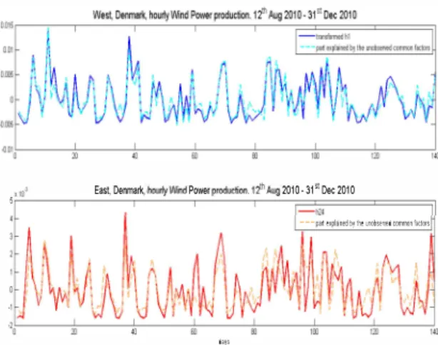
In Figure 6 we show how the series in Figure 3 and their main features are well resembled by the common factors estimated as detailed above. Just for illustration purposes we show this for the wind power production in hour 1 for West Denmark, and for hour 24 in the Eastern region.
! 10') Eas� DenmaI1c, hourtyWind Power production.12t1l Aug 2010 - 31st Dec 2010
5�---'---'--�-'�---'�-r============� -112.(
---�i:t ,lpll nEil Oj'th, u-;obs!;)l'd C(i:nrro�f;ctcrs
.,,;---;;---;;---;;;.---:c---;;;---;';c---�
d,ys
Figure 6. Part of the original series that is explained by the common factors extracted. Results for hour I in the West region (top) and hour 24 in the East
(bottom) .
Related to Figure 6, the difference between the series and the part of each one explained by the common components or factors are the so called specific components. They are stationary, which means they do not have unit roots (there is no need to take a difference on them to stabilize the mean). This implies that the forecasts of these specific components are only relevant when the forecasting horizon is really short. For longer ones the forecasts converge to zero (their mean).
IV. MID TERM FORECASTING OF HOURLY WIND POWER PRODUCTION
In this Section we will firstly describe the computational exercise carried out to check the performance of the proposed methodology in terms of forecasting accuracy.
We have dealt with the hourly data of both East and West regions in Denmark, from the 15t of January 2006 till the 29th of December 2012.
Forecasting with a Dynamic Factor Model, as proposed here consists of forecasting the common and specific components, and using equation (2) to compute the forecasts for Pt as follows:
A /'..�
PT+H =
0.j
T+H + eT+H,where T is the instant of time of the last day used to estimate the model and H represents the forecasting horizon, in our case this is 30 or 60 days.
We have considered 2 different historical lengths to estimate the models used to forecast: 15 and 20 weeks, without important differences between the forecasting results obtained. An open question for further research would be to carry out a computational experiment through which we can properly obtain the best historical length to use.
The forecasting experiment carried out consisted of using a rolling window of 15 weeks, and computing one-month-ahead forecasts with hourly disaggregation for the two regions, as well as two-months-ahead forecasts. Thus, one and two
month-ahead forecasts have been computed for every hour and day in this period. This makes our results reliable, since out of-sample forecasts have been computed for every day in a large span of years (2006, 2007, 2008, 2009, 2010, 2011 and the first two months in 2012).
The same experiment was done considering 20 weeks for the historical length of the data to estimate the models used to forecast.
Then, the Normalized Mean Absolute Error (NMAE) is computed for every hour and day. Given that the period for which the forecasts have been computed is so large, the conclusions obtained allows evaluating the validity of the proposed forecasting methodology4 to produce accurate mid term forecasts. The NMAE for a particular day d and hour h is defined as follows:
NMAE(h d)
=I �l,d - Ph,d I
,
Ie
d
'where
Ph,d
is the true hourly wind power production at hour h�
of day d, and
P h,d
is the forecast for this data.ICd
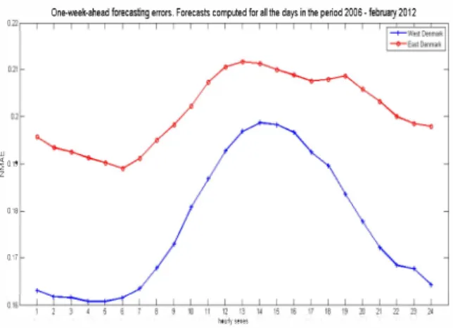
is the installed capacity at day d. This forecasting accuracy metric is one of the most well-known ones (read [4] for a revision on the accuracy metrics used in wind power forecasting).In Figures 7, 8 and 9 the NMAE for all the out-of-sample forecasts computed for every day in the period 2006 till the end of February 2012 with different forecasting horizons considered are shown, which are respectively 7 days, one month and two months.
w
One-week-ahead forecasting errors. Forecasts computed for ailihe days in the period 2006 -february 2012
O.22 ,--,---,----,--,---,--,,-'-T---.--,---,---,---,--,---,----,--,---,--,,--,-;=Ic==
�
0.19 0.18 0.17 a.'6L1�:-r-==L-!--+---!---+-�11---!-1l-C''-3 �"---+'5-C''-6 --c"1I--+,s-,o-g --!"--+l1---!-n -c,'-3 -+,,� hO\.�I"I�SFigure 7. NMAE. Oue-week-ahead forecasts.
4 (based on an existent econometric model, the Dynamic Factor Model, but
extended to be able to take into account the relationship between aggregated hourly productions in regions which are close to each other, and then affected by common meteorological circumstances)
w � 019
One-month-ahead forecasting errors. Forecasts computed for a1llhe days in the period 2006 - february 2012
1 2 1 � 5 6 7 8 9 10 11 12 13 14 15 16 17 18 Ig 20 21 II B 2�
w
� 0,19
Z
hoiJ1yserie,
Figure 8. NMAE. One-month-ahead forecasts.
One-week-ahead forecasting elTors. Forecasts computed for alilhe days in the period 2006 - february 2012
11 12 13 14
It�urltsenes
Figure 9. NMAE. Two-months-ahead forecasts.
The accuracy of the results obtained is demonstrated, and even clearer if compared with NMAEs around 0.08 and 0.1 for forecasting horizons of just I or 2 days, see [4] for a comparison with results obtained in these cases.
Additionally, the forecasting errors remain relatively stable, although extending the forecasting horizon from one week up to two months. This means that the model proposed captures adequately the level of the series under study, and capturing these levels is the key when extending the forecasting horizon so longer (2 months).
V. CONCLUSIONS AND FURTHER RESEARCH
In this work we present a methodology that is able to compute mid-term forecasts for the aggregated wind power production in an area or region with hourly disaggregation, which is a crucial task for all the agents involved in the operation of electricity markets. For instance, from the perspective of a wind power producer forecasts for these horizons could be useful to program the maintenance of the wind farms, selecting the most convenient period for this task.
To the best of our knowledge, till now there were no available procedures that were able to compute accurate
forecasts for recasting horizons longer than 48 or 72 hours. In that cases the NMAE were around 8 - 10%. Here, we obtain a NMAE of 17.72% for West Denmark when the forecasting horizon is 2 months, i.e. 1440 hours. For East Denmark we obtain an NMAE of 20.12%. These average errors were calculated for a large span of years (6 years and 2 months), which makes the conclusions trustable and significant.
Thus, the achievement of this work is the calculation of accurate mid term forecasts for wind power production. The methodology has been illustrated with the Danish data, but of course it is of application to any other country. Furthermore, this should be seen as a starting point for extending even further the forecasting horizons. They were not longer than a few days (usually 2 or 3 in previous works).
Interesting extensions of this work could be:
1. Carrying out a formal comparison of forecasting results depending on the length of the rolling window considered (historical data used to estimate the models used to forecast).
2. Using bootstrap techniques to calculate scenarios, i.e., not only point forecasts but also probabilistic ones. This can be done by following the ideas in [19]. The main idea is to generate bootstrap replicas of the common factors as well as bootstrap replicas of the specific ones. Then, generating bootstrap replicas of the original series, and re-estimating the model for each replica. This allows computing confidence intervals of all the parameters in the model. Then, to compute bootstrap-based forecasting intervals this scheme should be slightly modified to be able to replicate the condition distribution of future observation given the data.
3. Extending the forecasting horizons even longer, once that this methodology has been identified as a useful one in this direction.
REFERENCES
[ I ] Sanchez, L (2006a). Recursive Estimation o f Dynamic Models Using Cook's Distance with Application to Wind Energy Forecast.
TECHNOMETRlCS, 48, 1, 61-73.
[2] Sanchez, L (2006b). Short-term prediction of wind energy production.
International Journal of Forecasting, 22, 43-56.
[3] Sanchez, L (2008). Adaptive combination of forecasts with application to wind energy. International Journal of Forecasting, 24, 679-693. [4] Garcia-Lobo, M. (2010). Metodos de predicci6n de la generaci6n
agregada de energia e6lica. PhD Dissertation, Universidad Carlos 11/
de Madrid.
[5] Jonsson, T., Pinson, P and Madsen, H. (2010). On the market impact of wind energy forecasts. Energy Economics, 32, 2, 313-320.
[6] Pinson, P., Papaefthymiou, G., Klockl, B., Nielsen, H.A. and Madsen H. (2009). From probabilistic forecasts to statistical scenarios of short term wind power production. Wind Energy, 12, 51-62.
[7] Pinson, P. and Girard, R. (2011). Evaluating scenarios of short-term wind power generation, MIMEO, Technical University of Denmark. [8] Alonso, AM., Garcia-Martos, C, Rodriguez, 1 and Sanchez, MJ.
(2011). Seasonal Dynamic Factor Analysis and Bootstrap Inference Application to Electricity Market Forecasting. TECHNOMETRICS,53
(2), 137-151.
[9] Garcia-Martos, C, Rodriguez, J. and Sanchez, M.J (2011). Forecasting electricity prices and their volatilities using Unobserved Components.
Energy Economics.
[10] Garcia-Martos, C, Rodriguez, J. and Sanchez, M.J (2012). Forecasting electricity prices by extracting dynamic common factors: application to the Iberian Market. lET Generation, Transmission & Distribution.
[11] Lee R. D , Carter L. R. (1992). Modelling and Forecasting U S. Mortality. Journal of the American Statistical Association, 87, 419, 659-671.
[12] Ortega, J.A, and Poncela, P. (2005). Joint forecasts of Southern European fertility rates with non-stationary dynamic factor models.
International Journal of Forecasting, 21, 539-550.
[13] Pen a, D. and Box, GEP. (1987). Identifying a simplifying structure in time series. Journal of the American Statistical Association, 82, 399, 836-843.
[14] Stock, .I. H. and Watson, M. (2002). Forecasting using principal components from a large number of predictors. Journal of the American Statistical Association, 97, 1167-79.
[15] Harvey, A., Ruiz, E. and Sentana, E (1992). Unobserved Component Time Series Models with ARCH Disturbances. Journal of Econometrics, 52, 129-158.
[16] Papaefthymiou, G. and Pinson, P. (2008). Modeling of Spatial Dependence in Wind Power Forecast Uncertainty. PMAPS 'os.
Proceedings of the 10th International Conference on Probabilistic Methods Applied to Power Systems.
[17] Grady, W.M., Groce, LA, Huebner, T.M., Lu, QC and Crawford, M.M (1991). Enhancement, Implementation, and performance of an adaptive short-term load forecasting algorithm. IEEE Transactions on Power Systems.
[18] Kwang-Ho K , Hyoung-Sun Y and Yong-Cheol K. (2000). Short-term load forecasting for special days in anomalous load conditions using neural networks and fuzzy inference method. IEEE Transactions on Power Systems.
[19] Alonso, AM , Pena, D, Rodriguez, J. (2008). A methodology for population projections: an application to Spain. UC3M Working papers, 2008. Statistics and Econometrics Series. 08-12.