CHIRPS: Explaining random forest classification
Julian Hatwell1 · Mohamed Medhat Gaber1 · R. Muhammad Atif Azad1
© The Author(s) 2020
Abstract
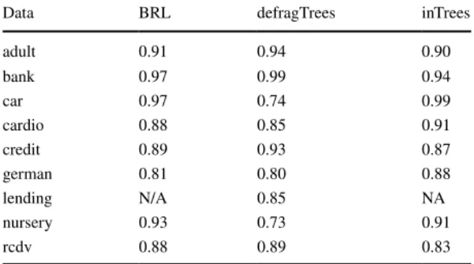
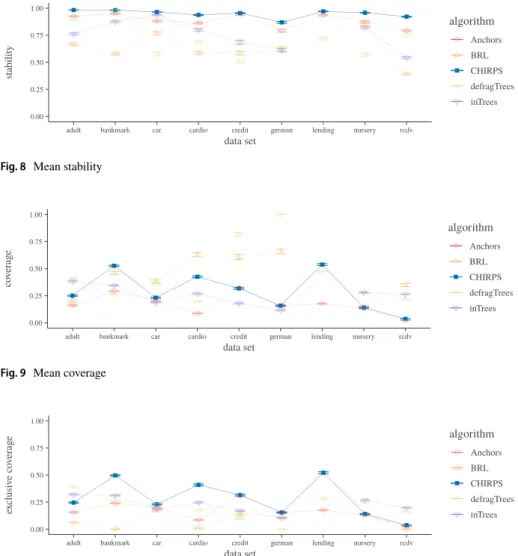
Modern machine learning methods typically produce “black box” models that are opaque to interpretation. Yet, their demand has been increasing in the Human-in-the-Loop pro-cesses, that is, those processes that require a human agent to verify, approve or reason about the automated decisions before they can be applied. To facilitate this interpretation, we propose Collection of High Importance Random Path Snippets (CHIRPS); a novel algorithm for explaining random forest classification per data instance. CHIRPS extracts a decision path from each tree in the forest that contributes to the majority classification, and then uses frequent pattern mining to identify the most commonly occurring split condi-tions. Then a simple, conjunctive form rule is constructed where the antecedent terms are derived from the attributes that had the most influence on the classification. This rule is returned alongside estimates of the rule’s precision and coverage on the training data along with counter-factual details. An experimental study involving nine data sets shows that classification rules returned by CHIRPS have a precision at least as high as the state of the art when evaluated on unseen data (0.91–0.99) and offer a much greater coverage (0.04– 0.54). Furthermore, CHIRPS uniquely controls against under- and over-fitting solutions by maximising novel objective functions that are better suited to the local (per instance) expla-nation setting.
Keywords XAI · Model interpretability · Random forests · Classification · Frequent patterns
1 Introduction
Explainable Artificial Intelligence (XAI) is no longer just a research question (Doshi-Velez and Kim 2017); it is a concern of national defence and industrial strategy (Gunning 2017; Goodman and Flaxman 2016) and a topic of regular public discourse (Tierney 2017; O’Neil and Hayworth 2018). The challenge—to make AI explainable—arises because of a cognitive-representational mismatch; modern machine learning (ML) methods and models operate on dimensions, complexity and modes of knowledge representation that make them
* Julian Hatwell
[email protected] http://www.bcu.ac.uk
opaque to human understanding. Such models are termed “black boxes” (Freitas 2014; Lipton 2016).
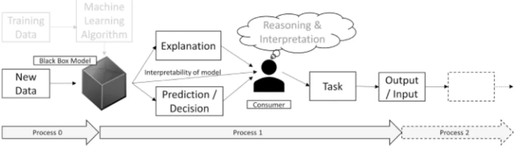
Some have argued that classification performance improves only negligibly when we use complex, black box models instead of the classical methods such as linear discri-minant analysis (Rudin 2018; Hand 2006); however, the majority still prefers to use the black box models such as Random Forests, Gradient Boosting Machines, Support Vector Machines and Neural Networks as the first choice methods for many applications. This preference may in part be thanks to the intense performance competitions—such as those hosted by Kaggle—as well as demands of commercial and critical applications. Research into these black boxes is motivated because they can achieve very high predictive accu-racy that makes them suitable for such critical applications despite an almost complete loss of interpretability (Burrell 2016; Pasquale 2015; Hildebrandt 2012). Yet, this accuracy-interpretability trade-off (AITO) poses a barrier to adoption of these most accurate models in regulated industries where sensitive and personal data are used to make life-changing decisions about individuals (Goodman and Flaxman 2016). Automated decisions from a black box model are difficult to contest or defend; organisations that rely on such unex-plainable decisions are at risk of non-compliance with data protection regulations (Euro-pean Parliament and Council of the Euro(Euro-pean Union 2018); moreover, organisations that fail to understand their automated decision making will not be able to identify or rectify mistakes and sources of bias. Black box models also face obstacles in the medical sector where automated diagnostics and personalised medicine offer untapped potential. Evidence in the literature shows that practitioners and clinicians are not yet ready to adopt models that do not provide clinical insight or do not easily align with prior knowledge, even if they are demonstrably more accurate. This lack of trust can impact negatively on patient outcomes (Jovanovic et al. 2016; Turgeman and May 2016; Letham 2015a; Subianto and Siebes 2007; Huysmans et al. 2006). XAI can improve trust where interpretation, interac-tion, intervention or expert verification by human agency is required. These scenarios can generally be described as Human-in-the-Loop (HIL) processes (DoD Modeling and Simu-lation (M&S) Glossary 1998), as illustrated in Fig. 1. A HIL process is any organisational process in which a human agent is required to complete a downstream task that depends on reasoning about an automated decision. HIL processes present a strong motivation for research in XAI and ML interpretability.
In this paper, we propose Collection of High Importance Random Path Snippets
(CHIRPS), a novel, heuristic algorithm that provides instance-wise explanations of ran-dom forest (RF) classification. A CHIRPS explanation is in the form of a classification rule, supplemented by estimated performance measures (e.g. precision and coverage)
Fig. 1 Process 0 represents submission of new data to the trained model for classification, Process 1 is a generic HIL process where the consumer must interpret the model output, and Process 2 is some down-stream task that relies on the consumer’s judgement
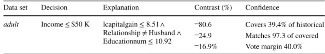
over the input space along with counter-factual detail. An example from the UCI Machine Learning Repository (Dheeru and Taniskidou 2017) adult data set is shown in Table 1. For this data set, the task is to build a model that can classify individuals according to whether they earn more or less than $50K annually. The individual shown was classified by a random forest model as having income ≤ $50K, and the CHIRPS explanation is a
combination of three attributes: insufficient (log) capital gain, not married, and education level <11 , which indicates that this individual lacks a college degree on this ordered cat-egory. The explanation is immediately interpretable in the context a denial of credit deci-sion, or similar downstream task. The Contrast column shows how far precision decreases when switching out each attribute term in the antecedent. This individual would surely receive a different result if they had saved more capital and, as such, this is an immedi-ately actionable result.
We show a second example in Table 2 using the rcdv data set (ICPSR1) relating to crim-inal recidivism in North Carolina during 1978 and 1980. For this data set, the task is to classify individuals as likely (“Y”) or unlikely (“N”) to reoffend. The individual shown has been classified as likely to re-offend. Without an explanation, the classification might not be called into question. However, the very dubious explanation White (race) = False is given, indicating that this single attribute was the deciding factor. In plain English, the model classified the individual as a risk of re-offending because they are African Ameri-can! With the full detail of the explanation, we can see that this attribute was a very poor indicator. The vote margin within the black box model was borderline, at best. The auto-mated decision taken about this individual appears to be little more than a random guess and worse still, this situation affects up to 20% of historical data. The explanation exposes serious flaws in the model itself, raising the necessity to reappraise the data set for bias, and to examine every stage of the model training. More broadly, this result highlights the ethical problems of relying on model classifications alone to make such life-changing decisions.
Table 1 An example of CHIRPS output for explaining an automated decision
Data set Decision Explanation Contrast (%) Confidence adult Income ≤ $50 K lcapitalgain ≤8.51 ∧
Relationship ≠ Husband ∧ Educationnum ≤10.92
−80.6 Covers 39.4% of historical −24.9 Matches 97.3 of covered −16.9% Vote margin 40.0%
Table 2 A further example of CHIRPS output, illustrating diagnosis of a poor performing model Data set Decision Explanation Contrast (%) Confidence
rcdv Recid = Y White = False −19.8 Covers 19.4% of historical Matches 50.0% of covered Vote margin 2.7%
To achieve these results, CHIRPS looks at the decision paths taken by the RF to classify a single instance (the explanandum) in each base decision tree (DT) classifier, and retains only those paths that formed the majority vote. This step is justified because a rule based explanation must be locally accurate, meaning that the rule consequent always agrees with the model’s classification (Lundberg and Lee 2017). The minority paths give a different classification and cannot form part of the explanation.
CHIRPS then employs Frequent Pattern (FP) mining to filter only the decision nodes that occur most frequently within the collection of decision paths. The most frequent nodes refer to attributes that contribute the most to the model’s classification. The nodes (or terms) are greedily added into a single classification rule (CR); only the terms that improve the performance against the objective function are added. The “Contrast” analysis in Tables 1 and 2 shows how the rule’s performance deteriorates when we exclude each individual term from the antecedent.
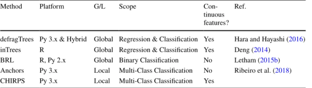
Our experimental study over nine data sets compares CHIRPS with four state of the art methods, that is, Anchors (Ribeiro et al. 2018), Bayesian Rule Lists (Letham 2015a, b), inTrees (Deng 2014) and defragTrees (Hara and Hayashi 2016). These methods generate a rule or cascading rule list (CRL), and so are directly comparable. They are also well cited in the literature. Our results show that CHIRPS is at least as good or significantly better in all quality measures in a comparative study that is broader in scope than much of the previ-ous work in this research area. Furthermore, CHIRPS works well in multi-class problems and class-imbalanced problems, where other methods are inconsistent. Unlike some com-peting methods, CHIRPS does not require discretisation of continuous features as a pre-processing step, and therefore works directly with the model under scrutiny (MUS). We further show that using the traditional objective functions for finding optimal classifica-tion rules—precision and coverage—leads to over- and under-fitting soluclassifica-tions. We suggest novel counterparts that perform better in the local explanation setting.
The remainder of this paper is organised as follows: Sect. 2 discusses related work; Sect. 3 covers key concepts of Decision Trees and Random Forest models; Sect. 4 formal-ises the general problem of explaining classification models and the requirements of an effective solution; Sect. 5 shows how classification rules can be extended to meet all the requirements of explanation; Sect. 6 presents CHIRPS; Sects. 7 and 8 detail our experi-ments and discuss the results; and finally, Sect. 9 concludes the paper and presents some ideas for further work.
2 Related work
In the last decade, many approaches have been taken to ML interpretability. There have been novel model types, designed for interpretability (Letham 2015b; Friedman and Pope-scu 2008; Riiping 2006; Waitman et al. 2006). The advantage of using such methods is early discovery of false assumptions and problems in the data set. Such methods can gen-erate a sparse model that takes advantage of domain knowledge (Rudin 2018). Another approach is to extract an interpretable approximation from an already trained, black box model (Adnan and Islam 2017; Hara and Hayashi 2016; Deng 2014). Although all the methods mentioned so far are very different in their implementation, very many of the resulting models fall into the general category of rule sets or rule lists, especially Cascad-ing (or fallCascad-ing) Rule Lists (CRL). This is because logical rules present an uncomplicated, semantic mapping between the inputs and outputs of classification and are considered by
many to provide the most intuitive explanations (Wang et al. 2017; Souillard-Mandar et al. 2016; Wang et al. 2016; Wang and Rudin 2015). CRL are ordered sets of classification rules (CR). CR are rules where the antecedent defines regions of the input space and the consequent is the expected class label in that region.
Bayesian Rule Lists (BRL) (Letham 2015a, b) and Brute (Waitman et al. 2006) are two well-known algorithms for generating a CRL directly from data. The objective is to create an interpretable model, as opposed to explaining an existing one. The complete set of CR is extracted from the data set and subjected to Frequent Pattern (FP) mining. Each method employs a probabilistic strategy to return a subset of mined rules of a user-defined, man-ageable size as the final model. Neither method modifies or constructs rules from sub-units. Aside from standard quality measures of the rules (precision and coverage), these methods provide a measure of uncertainty of the rule’s classification. Brute uses several rounds of bootstrapping of the training data to extract CR for the FP mining. Rules that are simi-lar and frequently occurring across replicates are retained, allowing antecedent terms with variance estimates. BRL, on the other hand, uses Monte-Carlo Markov Chains to return a distribution of rule lists. Individual rule lists from the chain can be used as spot estimates, or the distribution can output rules where the consequent is a probability distribution.
The RuleFit algorithm (Friedman and Popescu 2008) is notable for producing a novel rule-based model type, the predictive rule ensemble (PRE). The first step is to generate an intermediate specialised decision forest (DF). The maximum depth of each tree is a small, random integer, resulting in shallow decision trees with high variance that serve as a large pool of engineered, rule-based features. Next, a linear model (LM) is trained using all of the untransformed and engineered features together, while LASSO regularisation (Tibshi-rani 1996) ensures that the LM contains a minimal set of non-zero coefficients. These coef-ficients represent the contribution of the most important features. The rule-based terms in a PRE must be interpreted as oblique (non-orthogonal) parameters whose contribution is counted when the rule covers the instance. Questions remain about the interpretability of such oblique parameters in linear models (Huysmans et al. 2006).
Other methods generate a CRL as a proxy model from an existing MUS (that is always a DF of some kind), as opposed to learning directly from data. This approach is called
decompositional (Andrews et al. 1995) because it reduces the search to the smallest infor-mation units of the model (e.g. the inner decision nodes of each base classifier in a decision tree ensemble). The purpose of the proxy is to explain the MUS through a more inter-pretable, simplified structure. The challenge for this approach is to maximise fidelity with the MUS. The related literature shows that such simplified, proxy models inevitably give a classification result that differs from the MUS for a proportion of instances. This phe-nomenon is a consequence of the AITO and such proxy models cannot be used to com-pletely replace the original model. Less than perfect fidelity is a failure to explain individ-ual instances (Rudin 2018); a situation that is unlikely to be acceptable in compliance and safety critical applications. Well known methods in this category include RF+HC (Mash-ayekhi and Gras 2015), ForEx++ (Adnan and Islam 2017), defragTrees (Hara and Hayashi 2016) and inTrees (Deng 2014). Each of these methods extracts all possible rules from root to leaf of each tree in the DF. The inTrees framework then uses FP mining to identify fre-quently occurring rules, while RF+HC and ForEx++ score each rule and apply a heuristic to identify a reduced rule set and defragTrees uses a Bayesian formulation. Based on the experimental results given in the relevant articles, the rule lists for RF+HC and ForEx++ remain too large to be considered truly interpretable. However, the stated aim of ForEx++ is knowledge discovery rather than interpretability per se and the authors further analysed the rule sets for patterns and trends.
Until recently, the interpretability gains of CRL were stated and accepted without much critique (Lipton 2016). However, to classify an instance, a CRL requires a top down evalu-ation; several rules may need to be parsed before finding one that covers an explanandum instance. The resulting explanation is the conjunction of the relevant rule and all preceding rules. Sometimes, there is no covering rule in the list and the model must default to the prior majority class. The interpretation of this default condition is null, “don’t know,” or “the model decided class yk because this is true for the most instances.” It is a trivial and under-fitting result that is unlikely to be acceptable in compliance and safety critical appli-cations. To minimise these undesirable outcomes, a very long rule list may be required, reducing the comprehensibility of the CRL as a whole. So, CRL are straightforwardly interpretable only for easy to classify instances; those that are covered by a rule near the top of the list. A more realistic goal for CRL is to extract general and holistic insights about the model and data as stated in Adnan and Islam (2017), because they have significant dis-advantages for explaining individual classifications. Decision Set based models (Lakkaraju et al. 2016) overcome this limitation, by generating an unordered rule set. As such, a deci-sion set is an OR of ANDs where any one or more rules may resolve to true for an explana-dum (Malioutov and Varshney 2013). These models usually require a user-defined and/ or domain informed prior to control the rule cardinality and number of rules generated (Wang et al. 2015); however, the main challenge of these methods is to find the optimal set that maximises coverage while minimising overlap (multiple rules covering the same instances). Overlap requires a tie-break that introduces uncertainty into the classification, while lack of coverage causes a default classification. These problems were recorded on up to 14% of test instances (Lakkaraju et al. 2016), which would be considered much too high for critical applications.
More recently, local explanation methods have emerged that sidestep the AITO alto-gether. They simplify and generalise per instance classifications (Ribeiro et al. 2018; Lund-berg and Lee 2017; Ribeiro et al. 2016; Subianto and Siebes 2007). Local methods implic-itly acknowledge that it is untenable to present a human interpretable view of the entire space of a black box model’s behaviour (Lipton 2016). This approach allows the MUS to be tuned for optimal classification (or prediction) accuracy without being compromised by the explanation process; that is, there is no loss of fidelity. Several local methods have been proposed in a model-agnostic framework, probing the model’s behaviour without needing to access the internal representation. They learn how the model’s output changes over a perturbation distribution in the locality around the explanandum (according to some distance metric) and infer the importance of varying the inputs from the resulting output values. This approach, of learning from the model’s behaviour, is described as didactic
(Andrews et al. 1995). LIME (Ribeiro et al. 2016) is perhaps the most popular of these methods since its publication and recently Shapley values (Lundberg and Lee 2017) has also gained attention. These methods assign a real value to the most important attributes, hence are known as Additive Feature Attribution Methods (AFAM). An AFAM explana-tion is equivalent to a surrogate LM that approximates the behaviour of the classifier at the locality of the explanandum. The largest coefficients indicate largest contribution to the model’s classification or prediction. LIME and Shapley Value explanations are intuitive for the end user, thanks to well-designed graphical outputs. However, it is not easy to know when one instance’s explanation applies to other instances. This limitation was overcome in Anchors, which is a very recent extension to LIME. Anchors returns a single rule as an explanation, illustrating the enduring importance of logical rules despite the paradigm shift towards local explanations. Relevance of an explanation to other instances is deter-mined unambiguously; either the rule is covering the new instance or it is not. Anchors
and LIME require all features to be discrete, and internally pre-process any continuous features into quartile bins by default, which can result in loss of information. These tech-niques have been shown to be effective in image and text classification but there are some limitations when applied to tabular data sets (Michal 2019). As described in Ribeiro et al. (2018) and Ribeiro et al. (2016), the perturbation distribution must be estimated from the joint distribution of the source data and this requires access to the training data set. In other words, these model-agnostic methods are not data-agnostic! If access to the training set is assumed, then the model-agnostic assumption of accessing only the inputs and outputs of the black box model is violated. This problem is overcome in LORE (Guidotti et al. 2018), which uses a genetic algorithm to generate a population of instances and allows for a worst case scenario where only information about the permissible range of values for each fea-ture in the input space in known. This approach, however, is limited to binary classification and can take a prohibitively long time to run. Also, all of these local sampling techniques have been shown to introduce uncertainty and explanations with high variance for similar instances (Fen et al. 2019). This means they require additional checks to determine whether the selected attributes and features are stable over repeated trials. These results suggest that the model-agnostic assumption should be taken with caution.
We argue that the model-agnostic assumption is only required for a subset of problems in the context of HIL processes, such as model auditing by an external third party. HIL pro-cesses are frequently found in settings where the model and its training/test data are owned by the explainee. For example, a financial services company segmenting its loan applica-tions by risk, or a medical enterprise implementing automated diagnostics. In these cases, there is no imperative to use a model-agnostic method, especially if a different approach gives better insight. Another problem with model-agnostic is that they explain correlations in the synthetic sample, but not necessarily what the black box model computes (Rudin 2018). This problem calls for a decompositional approach that explains each data instance separately and reveals the internals of the black box.
The very notion of interpretability in ML has been frequently ill-defined in the ML lit-erature, with serious attempts at scientific rigour only appearing very recently (Doshi-Velez and Kim 2017; Bibal and Frenay 2016; Lipton 2016; Subianto and Siebes 2007). Taking an inter-disciplinary approach and drawing from the social sciences, Miller (2017) sets forth guiding principles for a form of explanation that reflects how people explain actions and reasoning to one another. Several other sources confirm that this is a desirable quality
(Woodward 2017; Wilkinson 2014; Salmon 1971; Hempel and Oppenheim Apr. 1948). These guiding principles suggest that explanations should be:
• minimally complete—neither under- nor over-fitting;
• contrastive—providing information about counter-factual cases;
• and a model of self—referring to historical data, not obscure parameters or synthetic distributions.
This research contributes a formalisation of explanations that align with these principles. Furthermore, our proposed method is the first explanation method to our knowledge that addresses directly the above principles. By relaxing the model-agnostic assumptions and given the realities of supervised learning on tabular data sets, our method offers the best of decompositional and didactic methods. Our rule-based explanations have no loss of fidel-ity, unlike global methods. When tested on unseen data and compared to state of the art methods, the rules are also more precise without tending to over-fit, and have higher cov-erage without tending to under-fit. These properties produce excellent robustness to class
imbalance where other methods struggle. Aside from LORE (Guidotti et al. 2018), ours is the only method to enhance the explanation with information about counter-factual cases but our method naturally addresses multi-class problems and classification uncertainty, while LORE only targets binary classification problems.
3 Decision trees and random forests
Before presenting our method in detail, we provide a brief overview of Decision Trees (DT) and, more specifically, the Classification and Regression Trees (CART) algorithm. CART models are the DT variant used in the original Random Forest (RF) algorithm (Bre-iman 2001). The CART algorithm is a heuristic method for inducing DT by top-down, greedy, recursive, and binary partitioning of the training data set. CART induction begins with a single (root) node that covers all training data instances. Using non-class attributes, CART proceeds by generating decision nodes that separate the instances into increasingly pure partitions according to their class label. On each iteration, candidate splits are evalu-ated for all nodes that are currently at the end of a decision path but do not yet meet the stopping criteria. The candidate split that would generate two child nodes with the lowest weighted total Gini Impurity IG is always chosen and those child nodes are then added to the growing tree:
where pk is the proportion of instances having label yk in a node Q and K is the number of classes.
where {Qfirst,Qsecond} is the set of child nodes that would be created by the candidate split and |Q| is the number of training instances covered by a node. This action occurs indepen-dently from any previous or subsequent iteration. There is no way to back out a previous move or find better splits by considering feature interactions. As such, this typifies a greedy heuristic; it is much more computationally efficient than an exhaustive search but has no guarantee of finding the optimal DT. The method is deterministic for a single tree and a static sample.
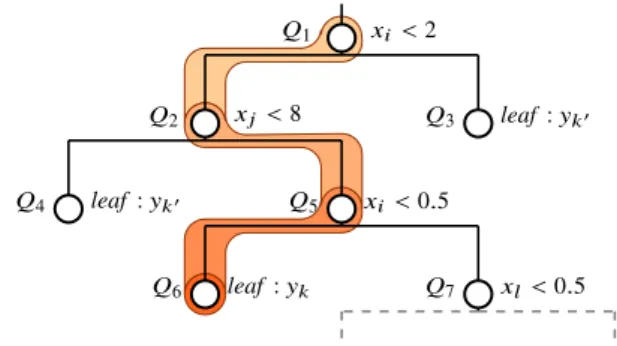
To classify a previously unseen instance, simply follow the path of that instance down the tree, beginning at the root and obeying the split condition of each decision node until a leaf node is reached. The split conditions are binary conditions that are either true or false for an instance. So, every instance can follow one and only one path, and arrive at one and only one leaf node. Each leaf node covers a subset of the training instances and returns the majority class label of those instances as the classification. See Fig. 2.
A RF is an ensemble of, typically, tens to thousands of base DT classifiers. The ensemble operates in parallel and classifies by majority vote. This improves classifica-tion performance in an ensemble compared to a single classifier, assuming each classi-fier in the ensemble performs somewhat better than a random guess and they are diverse (if not completely uncorrelated) in their errors. In an ensemble, erroneous classifica-tions are outnumbered by correct classificaclassifica-tions with very high probability, resulting in
(1) IG(Q) = K ∑ k=1 pk⋅(1−pk) (2) Weighted TotalIG=IG(Qfirst)⋅|Qfirst|
N +
IG(Qsecond)⋅|Qsecond|
a correct classification on aggregate. To promote the required structural diversity among the base classifiers, stochastic processes are introduced at two stages of DT induction. Firstly, each DT is induced on a uniform sample with replacement (bootstrap) of the training data set. Secondly, although it is still always the best IG scoring candidate split that is added to the tree on each iteration, the candidate splits are limited to a ran-dom sub-sample of possible candidates. In other respects, tree induction is the same as described in earlier paragraphs except, to further increase the structural variance, it is common to avoid applying any stopping criteria. Under these conditions, trees are fully grown so that their leaves are pure; each leaf covers training instances of only a single class. The resulting trees can be very deep and bushy and individually over-fitting yet, as an ensemble, RF models constructed this way are highly competitive for accuracy among widely available ML methods (Fernandez-Delgado 2014) and are also robust to over-fitting (Breiman 2001), class imbalance, noise, non-informative features, anoma-lies and variations in the source data (Vens and Costa 2011), and more able to discover useful feature interactions over the whole sample of random trees. There are only two tuning parameters that control most of the variation in performance: the number of trees and the number of candidate features used to generate candidate splits. These proper-ties make RF easy to deploy and popular in practice. In contrast to the relatively simple structure of an individual DT, the consensus is that RF are typical examples of uninter-pretable, black box models; Breiman, the inventor of the original RF, described them as “impenetrable” (Breiman 2001). There are several methods for extracting a general measure of feature importance (Gain, Split Count, Permutation Error) but these deliver inconsistent results (Lundberg et al. 2017). Furthermore, these measures can only com-municate that certain features were more useful in delivering the model’s overall accu-racy or error scores. This falls short of providing explanations that detail the contribu-tion of specific attribute values to the classificacontribu-tion output or determining the effect of changing the inputs to generate counter-factual classifications.
4 Problem formulation
Interpretability of ML models has been poorly defined in the ML literature until recently (Lipton 2016). In response, this section presents our requirements for local explana-tions, based on the guiding principles proposed in Miller (2017). We also scope these definitions to classification problems on tabular data sets.
Fig. 2 To classify an instance 𝐱= {…,xi=0.1,xj=10,…} , we start at Q1 and follow the binary split conditions until we reach a leaf node, Q6 in this case, which returns the label yk to the caller
4.1 The problem of classification
Let X∈ℝP be a feature space where P∈ℕ is an arbitrary number of features. The jth feature is Xj . An instance space 𝐗∈X of N∈ℕ instances is an N×P matrix. Instance 𝐱(i) = [x(i)1 ,…,x
(i)
P] is the ith row vector of 𝐗 and 𝐗j= [x (1) j ,…,x
(N) j ]
T is the column vec-tor of the jth feature. An attribute x(i)
j is the value at the j
th feature of the ith instance. Let Y= {y1,…,yK} be the space of K possible class labels, and 𝐘∈Y be a vector of length N of known instance labels. There is an unknown, conditional distribution f =F(y|𝐱) such that any randomly sampled, labelled instance space (𝐗,𝐘) has the joint distribution F(𝐱,y) =F(y|𝐱)⋅F(𝐱) . A classifier is a known function g∶X⟼Y, g∈G selected from the hypothesis space G by empirical risk minimisation (Vapnik et al. 1998) over a given, labelled instance space (𝐗,𝐘) , such that g approximates f and is expected to generalise to any random instance space, sampled from the same distribu-tion: g(𝐗) ≈f(𝐗), 𝐗∈X
4.2 The problem of explaining classifications
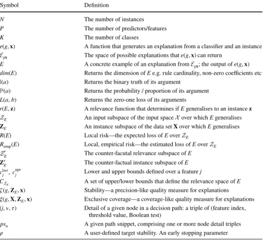
In Sect. 5 we will show that CR suit explanations; however, CR may not be the only valid or useful choice. Therefore, in this section we first build a theoretical framework for expla-nations in general. To aid the reader, we provide Table 3 as a key to the notation used that introduces new concepts in the remainder of this article.
We seek a function e∶G,x⟼E whose output is E=e(g,𝐱),E∈Eg𝐱 , where Eg𝐱 is the space of possible explanations for a single black box classification event g(𝐱) . E must be optimal for reliability, generality and interpretability. The trade-off between reliability and generality weighs upon most ML research but interpretability adds several dimensions. It is very difficult to define a general form for explanations that could apply to all situations (all hypothesis spaces and problem spaces). Measuring whether and how much a given E is informative requires the use of proxies that can only be compared between solutions of the same class, such as the number of non-zero linear coefficients (linear models), rule cardi-nality and number of rules (rule-based models), maximum tree depth or number of nodes (decision trees), number of support vectors in SVM (Bibal and Frenay 2016; Garcia 2009), or the number of relevant features from a tabular data set. This is not always satisfactory in high dimensional problems (Lipton 2016).
We identify the following requirements:
Requirement 1 E must be minimally complete. We want E to have the smallest possi-ble dimension dim(E) (perhaps measured as the above mentioned proxies). This require-ment means that E must be the smallest subset of useful information encoded in (g,𝐱) that maximises both reliability and generality. Consider, however, a classification task with class imbalance. A trivial or null explanation—one that states that the majority class was selected but gives no reasoning—could apply to every instance (maximum generality) and be valid for all the instances that receive the majority class label from the model (very high reliability). This situation is erroneous because it explains the classification event without any reference to the model’s encoding of attribute differences between the classes—the relationship between 𝐗 and 𝐘 . The implication is that all input values lead to the target
class, which is false. This is an under-fitting scenario, equivalent to a classification model with constant output. So, E must reduce the problem dimensionality but must remain informative to some extent; E may not be trivial.
Requirement 2 There must be some function r that determines when E=e(g,𝐱) is rel-evant to any instance other than the explanandum instance 𝐱 in the reduced dimension of the solution space Eg
𝐱 (Req 1):
where 𝐳≠𝐱 , 𝐳∈X and a⊧b ( a models b ) means a is a logical conjunction and every part of a is true of b. Thus, the relevance subspace of E can be determined from r:
Note, E∈Eg𝐱 means that E is an explanation of 𝐱 , therefore r(E,𝐱) =1 and 𝐱∈ZE are always true.
(3) r(E,𝐳) = { 1 ifE⊧𝐳 0 otherwise (4) ZE= {𝐳∶r(E,𝐳) =1, 𝐳∈X}, ZEis continuous.
Table 3 Summary of notation
Symbol Definition
N The number of instances
P The number of predictors/features
K The number of classes
e(g,𝐱) A function that generates an explanation from a classifier and an instance Eg
𝐱 The space of possible explanations that e(g,𝐱) can return
E A concrete example of an explanation from Eg𝐱 ; the output of e(g,𝐱) dim(E) Returns the dimension of E e.g. rule cardinality, non-zero coefficients etc 𝕀(a) Returns the binary truth of its argument
ℙ(a) Returns the probability / proportion of its argument L(a, b) Returns the zero-one loss of its arguments
r(E,𝐳) A relevance function that determines if E generalises to an instance 𝐳 ZE An input subspace of the input space X over which E generalises 𝐙E An instance subspace of the data set 𝐗 over which E generalises R(E) Local risk—the expected loss of E over ZE
Remp(E) Local, empirical risk—the estimated loss of E over ZE Z′
E The counter-facutal relevance subspace of E 𝐙′E The counter-factual instance subspace of E clwr
j ,c upr
j Lower and upper bounds defined over a feature j
CZE A set of upper/lower bounds that define the relevance space of E 𝜁 (g,𝐙E,𝐱) Stability—a precision-like quality measure for explanations 𝜉(g,𝐗,𝐙E,𝐱) Exclusive coverage—a coverage-like quality measure for explanations (j,𝜈,𝜏) Detail of a given node in a decision path: a triple of (feature index,
threshold value, Boolean test)
psn A given path snippet, comprising one or more node detail triples 𝜌 A user-defined target stability. An early stopping parameter
Requirement 3 E must have maximal local reliability. The term local refers to everything inside the relevance subspace. Perfect local reliability means that g(𝐳) =g(𝐱),𝐳∈ZE but this may not be possible while simultaneously satisfying minimal completeness. We can proceed by minimising local risk:
Typically in ML research, the true distribution of 𝐳 is unknown. Therefore, the risk must be estimated empirically from an instance space 𝐗 of observed data. 𝐗 could be the train-ing set used to train g or any i.i.d. random sample from the same distribution. The relevant instance space is:
Then, empirical local risk can be estimated by:
which is related to precision, by way of reversing the zero-one loss function:
where the final term is equivalent to the standard definition of precision.
Requirement 4 E must be as general as possible given maximal local reliability. This means its relevance subspace covers the largest continuous volume of the feature space that achieves the same precision or better than any other relevance subspace. The E that satis-fies this requirement meets the following criteria:
Requirement 5 E must not be tautological, meaning that it generalises to a set of instances not limited to the singleton explanandum 𝐱 . An E that does not generalise beyond the sin-gleton 𝐱 is an erroneous situation that trivially explains the classification event g(𝐱) by the uniqueness of 𝐱 in the data set. This is the local explanation equivalent of over-fitting. Such over-fitting could arise at a complex or noisy decision boundary. In the most extreme case, where g(𝐱) =yk while for every near neighbour g(𝐳)≠yk , equation (8) is trivially max-imised if 𝐱 is the only member of 𝐙E and plummets when any 𝐳≠𝐱 is included in 𝐙E . In Sect. 5, we introduce a novel objective function, stability to gracefully handle this problem. (5) R(E) = ∫ L ( g(𝐳),g(𝐱))d𝐳, 𝐳∈ZE,E∈Eg𝐱, (6) L(a,b) = { 0 ifa=b 1 ifa≠b (7) 𝐙E= {𝐳∶𝐳∈ZE∩𝐗}. (8) Remp(E) = 1 |𝐙E| |𝐙E| ∑ i=1 L(g(𝐳(𝐢)),g( 𝐱));𝐳(𝐢)∈𝐙E, E∈Eg𝐱, (9) ℙ(g(𝐳(i)) =g(𝐱))=(1−Remp(E)
) = 1 |𝐙E| |𝐙E| ∑ i=1 1−L(g(𝐳(𝐢)),g( 𝐱)) = 1 |𝐙E| |𝐙E| ∑ i=1 𝕀(g(𝐳(𝐢)) =g( 𝐱));𝐳(𝐢)∈𝐙E, E∈Eg𝐱 (10) |𝐙E|>|𝐙E�|,ℙ ( g(𝐙E) =g(𝐱))≥ℙ(g(𝐙E�) =g(𝐱) ) ,E≠E�, E,E�∈Eg 𝐱.
Requirement 6 It must be possible to present E with contrastive, counter-factual informa-tion. That is, we assume that the form of explanation reveals the minimal changes to the inputs that give different results. In Sect. 5 we show how this is defined for CR specifically. Some authors posit that the counter-factual cases are any changes in the attributes of an instance that would result in a different classification (Guidotti et al. 2018; Subianto and Siebes 2007). However, such a definition can only apply to discrete, nominal and deter-ministic predictors. In the case of continuous predictors with complex decision boundaries, such as the mixed Gaussian process shown in Fig. 4, there could be several non-contigu-ous or interleaved regions of the input space (Ho and Basu 2002) that classify identically; in these cases a change of the minimal attribute set may not always result in a different class assignment. We can, however, expect a change in precision outside the relevance space and there is support for such models that offer measures of uncertainty rather than crisp boundaries in the literature (Proenca and Leeuwen 2019; Letham 2015a, b; Wait-man et al. 2006). Therefore, we propose a task dependent definition of contrastive explana-tions: counter-factual cases should be demonstrably different from observed cases. This difference is manifested as a drop in precision below some user-defined tolerance 𝛿 . That is ℙ(g(𝐙�
E) =g(𝐱) )
≤ℙ(g(𝐙E) =g(𝐱))− 𝛿 where
This quantity is the precision of the counter-factual instance space 𝐙′ E , and Z
′ E is the counter-factual relevance space. Note, Z′
E is a space, or set of spaces covered by minimal changes to E. It is not equivalent to {𝐗⧵ZE} , which is the entire input space not covered by E. If the latter were true, then each unique explanation would be a global model describ-ing the entire input space by itself and its complement. Rather, the benefit of counter-fac-tual information is to identify the boundary outside which E is no longer reliable.
Requirement 7 E should be a “model-of-self” that explains the model from the data. Model g is the output of a learning algorithm (a function) that was parameterised by the training data (𝐗,𝐘) . E should frame the explanation in terms of the influence of (𝐗,𝐘) over the original learning algorithm. This requirement is met de facto by the empirical formula-tions given.
In the following sections, we show how CHIRPS using CR as the form of explanation, is designed to meet these requirements. As our experimental study shows, competing meth-ods that do not explicitly address them all have a tendency to converge to under- or over-fitting solutions.
5 Extending classification rules as explanations
Frequent Patterns (FP), Association Rules (AR) and Classification Rules (CR) are all modes of expressing relationships between patterns in a data set. A pattern is formed from k≥1 attributes, and referred to as a k-item set. The support count= 𝜎(fp) is the number of
instances in a data set that match the pattern fp, while support(fp) = 𝜎(fp)
N is the fraction of instances containing fp. A pattern is said to be frequent if its support exceeds minsup, a user-defined threshold. AR describe associations over the whole data set between
(11) ℙ(g(𝐙�E) =g(𝐱))= 1 |𝐙� E| |𝐙�E| ∑ i=1 𝕀((g(𝐳(i)) =g(𝐱))), 𝐳(i)∈𝐙�E,𝐙 � E= {𝐳∈Z � E∩𝐗}
individual items within a k>1 item set. For example, for a 2-item set fp= {Z,Y} , there is a relationship expressed as the rule: Z ⟹ Y . Here, Z is called the antecedent and Y the consequent. Such an AR has a level of confidence or precision, which is equal to the condi-tional probability ℙ(Y|Z) = support({Z,Y})
support(Z) , where support(Z) =ℙ(Z) is the support of the antecedent alone (also called the coverage). A CR is simply an AR where Z is a set of con-ditions defined on one or more features {X1,…,XP} of a data set, and Y is a class label. It is trivial to derive a CR from the decision path of a DT (Quinlan 1987): Using the example from Fig. 2, the following is a CR:
5.1 Meeting the requirements for explanations
We can find CR that conform to our formulation of an explanation, given in Sect. 4, if we set Z=ZE , a relevance subspace, and Y=g(𝐱) , the output of the model. Then, the CR is
simply ZE ⟹ g(𝐱) . Req 2 is satisfied by this formulation because we can define the rel-evance evaluation function as:
where CZ
E is the set of parameters that define the lower and upper bounds of each feature. For a feature space with P features, any {clwr
j , c upr
j , j∈P} may be undefined, in which case the interval begins and/or ends with the domain of Xj . Minimising dim(E) requires |CZE| to be as small as possible, though it may not be zero (Req 1). The best case is |CZ
E|=1 and the worst case is |CZ
E|=2P.
To find candidates E∈Eg𝐱 that meet the requirements, we propose an iterative, breadth-first search heuristic as follows: at iteration i=0 , E(i) is a trivial or empty rule. In other words, the antecedent CZ
E(0) = ∅ while the consequent is g(𝐱) . Thus coverage is complete at the start and will be iteratively reduced in a trade off (Req 4) with precision. In each subsequent iteration i+1 we either add a new parameter or update an existing one that strictly increases the precision. However, to avoid tautological solutions (Req 5), we cannot use high precision as an optimisation target for this procedure because this measure can be trivially maximised with singletons or very small, overfit subspaces. We therefore propose
stability, a novel objective function that penalises explanations that explain only a small number of instances.
Definition 1 Stability takes the form 𝜁 ∶G,X,x⟼ℝ∈ (0, 1).
where K is a regularising constant and equals the number of possible classes.
The middle formulation in equation (14) shows how this measure relates to requirement 5; we calculate the precision of g(𝐳) =g(𝐱) inside the relevant instance space, excluding (12) {𝐱∶min(Xi)≤xi<0.5, 8≤xj≤max(Xj)} ⟹ y k (13) r(E,𝐳) ∶= P ∏ j=1
𝕀(max(clwrj , min(Xj))≤zj≤min(cuprj , max(Xj))), clwrj ,cuprj ∈CZE,𝐳∈X (14) 𝜁 (g,𝐙E,𝐱) = |{𝐳 ∶ g(𝐳) =g(𝐱), 𝐳∈𝐙E⧵𝐱}|+1 |𝐙E|+K = |{𝐳 ∶ g(𝐳) =g(𝐱), 𝐳∈𝐙E}| |𝐙E|+K
𝐱 itself. We apply additive smoothing as n+1
m+K . Then, the numerator simplifies as shown in
the final form. Therefore, stability is similar to using precision with a Laplace correction (Clark and Boswell 1991) but with a more severe penalty. Due to the division by K, trivial relevance spaces (of size 1) only get a stability of 33% or less for K≥2 . The function pro-file shown in Fig. 3 makes this clear.
We illustrate the benefit of this novel function with an example given in Table 4. At iteration i, there are twenty-one covered instances 𝐳∈𝐙E(i) . For all but one of these
g(𝐳) =g(𝐱) . This could be an optimal solution but the search continues to iteration i+1 . The rule takes a new, more specific parameter and 𝐙E(i+1) now covers just one instance. If
we are optimising for precision, E(i+1) would be considered better than E(i) because preci-sion is trivially maximised to 1.0. Stability, on the other hand, has fallen well below any tolerable level, so instead we keep E(i) as the explanation. It is important to realise that better recognised statistics such as recall and F-1 measure are unsuitable in this setting; since, the table shown in the examples is not a confusion matrix. Rather, we have tabu-lated the instance classification versus the rule coverage. We seek to maximise covered, target class and minimise covered, other class. We can tolerate high numbers of instances in the not covered column because we assume these instances will be covered by another explanation. Another perspective is that stability approaches precision asymptotically Fig. 3 Maximum achievable stability (the discrete points) when all instances are given the same classifica-tion, for relevant instance spaces containing from one to forty instances and K∈ {2, 3, 4} . The dashed line shows precision, which is always exactly 1.0 in these circumstances, no matter how small the instance space Table 4 Demonstrating stability
for K=2 with examples Rule-instance table Measure Values
Covered Not covered Iteration i
Target class 20 780 Stability 0.870
Other class 1 199 Precision 0.952
Recall 0.025
F−1 0.049
Iteration i+1
Target class 1 799 Stability 0.333
Other class 0 200 Precision 1.0
Recall 0.001
as |𝐙E|→∞ but when |𝐙E| diminishes so does the maximum stability; maximum stability = 1
K when |𝐙E|=1 . This behaviour acts as a brake that prevents the algorithm
from adding more parameters and converging on singletons. This is achieved non-paramet-rically, without the need for user intervention.
We introduce another, novel quality measure by returning to the minimal complete-ness requirement (Req 1). This states that there must be at least one informative parameter that can distinguish between differently classified instances. In situations of severe class imbalance, precision and coverage could simultaneously be trivially maximised by a null
solution that covers the entire input space. As we show in our experimental results, class-imbalance can lead to such under-fitting solutions in several competing methods. To guard against this, we propose a further, novel objective function, exclusive coverage in equation (15) that penalises high coverage against a lack of discrimination between classes.
Definition 2 Exclusive coverage takes the form 𝜉 ∶G,X,X,x⟼ℝ∈ (0, 1) . Exclusive coverage is calculated as coverage, the fraction of all instances covered by the rule exclud-ing the explanandum. This is similar to the relation between stability and precision. Addi-tionally, however, the value is weighted by the ratio of not covered, other class to not cov-ered, other class + covcov-ered, other class (equivalent of “true negative rate”). This measure increases with the number of differently classified instances outside the relevant instance space 𝐙E.
where TNR is the so-called “true negative rate” described above.
We illustrate the benefit of this novel function with an example given in Table 5. In this highly imbalanced class example, at iteration 0, the null rule covers all instances. Precision and stability are very high, perhaps above a threshold that could trigger an early stopping condition. Coverage is trivially maximised at 1.0. To report such a result would lead to a misleading representation of the rule quality. It is clearly an under-fitting solution. So we must add a term to the rule, even one that may dramatically decrease stability, precision and, of course, coverage. An example of a possible subsequent state is shown at iteration 1. At this point, the search for additional rule terms that can increase stability should con-tinue. So, at iteration 2, another rule term is added. This results in a more specific rule that has slightly reduced coverage, but slightly increased exclusive coverage. This example shows how using exclusive coverage as a quality measure helps to disqualify under-fitting solutions.
We reiterate the importance of using appropriate quality measures for explanations and how these differ from measures typically associated with classification accuracy (precision, recall, F-1 score). These novel functions are central to the contribution of this research. 5.2 Providing contrastive and counter‑factual information
Counter-factual examples illustrate changes in the inputs that will give different results. We have defined this in Req 6 as ensuring that the MUS’s outputs are demonstrably different (15) 𝜉(g,𝐗,𝐙E,𝐱) =TNR⋅ | 𝐙E⧵𝐱|+1 |𝐗|+K =TNR⋅ | 𝐙E| |𝐗|+K , 𝐙E⊆𝐗 TNR= |{𝐳 �∶ 𝐳�∉ (𝐙E) ∧g(𝐳�)≠g(𝐱)}| |{𝐰∶𝐰∈ (𝐗) ∧g(𝐰)≠g(𝐱)}|
for instances in the counter-factual space Z′ . This contrastive output may be a change of class label, or a significant drop in precision, that is, confidence in the given classifica-tion. Recall that the motivation for implementing local, per instance explanations is to avoid generalising the output of the MUS (model g) for the entire input space. We seek an explanation that is valid in the locality of the instance and we seek to avoid developing a global proxy of the MUS with all the disadvantages discussed in Sect. 2. The minimal completeness criterion means that it is necessary to show a decrease in precision below a user-defined tolerance only for spaces defined by a change to a single parameter in CZ
E , all others remaining identical. To obtain the complete set of adjacent spaces, we switch the position of each parameter c∈CZE , one at a time, such that a c
upr
j replaces c lwr j or vice
versa. This is illustrated in Algorithm 1 and visually in two dimensions in Fig. 4 where an unseen instance 𝐱 is classified as belonging to the triangle class. A candidate explanation, the optimal relevance subspace ZE= {𝐳∶a≤z1≤b, c≤z2≤d} is defined around 𝐱 by the parameters {a,b,c,d} . If the intervals [a, b] or [c, d] are any wider, there will be a drop in precision. If the intervals are any tighter, coverage decreases without improving preci-sion. By Algorithm 1, the adjacent (counter-factual) spaces are:
(16) Z� E= { A= {𝐳∶z1≤a,c≤z2≤d}, B= {𝐳∶b≤z1,c≤z2≤d}, C= {𝐳∶a≤z1≤b,z2≤c}, D= {𝐳∶a≤z1≤b,d≤z2}} Table 5 Demonstrating
Exclusive Coverage with Examples for K = 2
For clarity, we have included the TNR which is the ratio bottom left/bottom row total. The unweighted, intermediate term (not shown) is identical to coverage at three decimal places
Rule-instance table Measure Values Covered Not covered
Iteration 0
Target class 950 0 Stability 0.948
Other class 50 0 Precision 0.950
TNR 0.0
Excl. Cov. 0.0 Coverage 1.0 Iteration 1
Target class 200 750 Stability 0.881
Other class 25 25 Precision 0.889
TNR 0.5
Excl. Cov. 0.112 Coverage 0.225 Iteration 2
Target class 190 760 Stability 0.918
Other class 15 35 Precision 0.927
TNR 0.7
Excl. Cov. 0.143 Coverage 0.205
Provided the precision of the explanations representing each of these subspaces falls below the user-defined tolerance, all the requirements are satisfied. If a counter-factual space has a precision above the tolerance, the space can be merged with ZE by removing the defining parameter from the rule antecedent.
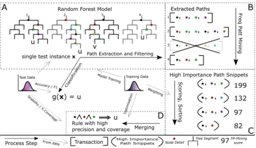
6 CHIRPS
We propose our novel procedure to search for CR that meet the requirements for local explanations. CHIRPS is a concrete implementation of the function e(g,𝐱) and the heu-ristic search introduced in Sects. 4 and 5. CHIRPS assumes g is a random forest model, which defines CHIRPS as a model-specific method. Each step is illustrated in the con-ceptual diagram in Fig. 5 and detailed in the following sections. To explain the clas-sification of an unseen instance, the original training set can be used in the rule finding step. The test set, originally used for assessing the classification accuracy of g, can be used to verify quality of the resulting explanations, using a leave-one-out procedure: One instance is classified and explained, while the remaining instances are kept aside and contribute no information to the explanation. These remaining instances can then be Fig. 4 A model with a complex boundary trained on a synthetic data set which has two classes, shown as triangles and circles and the candidate relevance space ZE is defined by four parameters a, b, c and d
used to determine stability and exclusive coverage scores for that individual rule. Thus each instance of the test set constitutes an experimental unit. Performance of an expla-nation algorithm is then the aggregate score over all these units.
6.1 Path extraction and filtering
The first step is to classify the explanandum instance 𝐱 and simultaneously extract the decision path of every DT. This is simply a matter of tracking the detail of each node. Without loss of generality, the node detail can always be posed as the evaluation of an inequality xj< 𝜈 , where j is a feature index and 𝜈 ∈ℝ . Let 𝜏 ∈ {0, 1} be the binary truth of the evaluation. Thus, each node detail is the triple (j,𝜈,𝜏) . Assuming nominal values are binary encoded, we can represent node detail for any data type with this structure. The interpretation depends on the domain of Xj . The following examples are for illustra-tive purposes and are non-exhausillustra-tive:
There is only one possible path for 𝐱 down each tree so the rest of the model is ignored (of course, for a different instance, a different set of paths are extracted). Trees have a number of nodes in O(2n) where n is the maximum tree depth, compared to paths that are O(n) , so this step reduces the search space logarithmically while retaining all the information about g(𝐱) . A second level of filtering is achieved by retaining only decision paths that agreed with the majority vote. Trees that voted for a minority class represent noise in the model. Their contribution was made redundant by the majority vote system.
(17)
(i, 0.5, 1) ∧Xi∈ {0, 1} ⟹ xi=0(binary false)
(j, 0.5, 0) ∧Xj∈ℝ ⟹ 0.5≤x
j≤max(Xj) (real valued interval)
(l, 3.5, 0) ∧Xl∈ {1, 2, 3, 4, 5} ⟹ xl∈ {4, 5} (likert score≥4)
Fig. 5 Conceptual diagram of CHIRPS in four steps: A. Path Extraction and Filtering, B. FP Mining, C. Scoring and Ranking, D. Merging and Pruning
6.2 Frequent pattern mining
In this section, we explain how FP mining is very well suited to extracting knowledge from random forests. Treating the RF model as a sample of a tree-structured random variable, certain stochastic phenomena have been demonstrated (Paluszynska 2017; Louppe 2017; Biau 2012; Vens and Costa 2011; Ishwaran 2007). As described in Sect. 3, CART adds decision nodes to a growing tree that minimise the total, weighted IG score on each itera-tion. Therefore, features with the greatest power to discriminate between classes occur with greatest probability at shallow levels because they are selected whenever they appear as candidates. This results in a smaller mean depth of nodes involving those features. Every root node in the RF has probability p=1 of being included in the set of decision paths of any instance. The probability of being included falls exponentially with each tree level because the number of alternative paths grows at O(2n) for n levels. So nodes involving the most discriminating features will appear in the collection of paths with very high probabil-ity. Also, the weighted total IG of a candidate split is conditional on all nodes above it in the same path. This means that features that interact have a greater chance of co-occurring in any given path, with these co-occurrences showing increased frequency over the whole collection. These properties suggest that frequency based filtering will be very effective at selecting the most important decision nodes. Furthermore, instances with more attributes in common are more likely to follow a similar path through each tree, resulting in solutions that are highly generalisable.
In addition to the above properties, note that FP mining requires a transaction list as input. A transaction list is a very suitable representation for the set of extracted and filtered decision paths. Each decision path can be considered as a transaction. Each transaction is a set of items, being the triples (j,𝜈,𝜏) described in the previous section.
The whole triple is the underlying unit for pattern matching. To execute a reasonable FP-mining task of these units, it is necessary to resolve the potentially very large num-ber of unique values resulting from real-valued features. The cut-point 𝜈 chosen inde-pendently by each DT might be anywhere in a location that separates the classes. That is to say, many unique values may all represent the same decision boundary. So, this uniqueness presents a problem. Before performing the FP mining, all triples matching (j,∙,𝜏)—where ∙ is any value—are discretised. This is illustrated in Fig. 6. Increasing Fig. 6 Simulation of discretising by the median (solid line) of twenty axis aligned splits (dashed lines) that all represent the same decision; they are sampled uniformly from inside the margin between two clusters that are linearly separable on continuous feature X1
the number of discrete values may improve results with more complex boundaries, so we use a binning function where number of bins can be set as a user-defined tuning parameter.
The output of FP mining is a list of FP that exceeded the minimum support, further filtering the search space prior to the rule building step. The support value of each item set is also returned as a score. Since these k-item sets may represent non-contiguous nodes in a path, we name these objects high importance random path snippets or sim-ply, path snippets.
6.3 Ranking
Even though the previous two steps have dramatically reduced the search space, find-ing the minimal set of snippets that maximises stability and exclusive coverage is a multi-objective, combinatorial problem. To avoid an exhaustive search we rank the snippets according to a heuristic score. The RF+HC method (Mashayekhi and Gras 2015) also uses a score function for rule ranking, so that function was considered first. Unfortunately, it demonstrates undesirable behaviour for our needs. Firstly, the penalty increases with rule length because rule length appears in the denominator. This is the wrong direction because, under FP mining, higher cardinality snippets naturally have lower support than those with lower cardinality (Agrawal et al. 1994). Those longer snippets that have passed our support threshold contain the most useful feature inter-actions. Secondly, the penalty depends on rule accuracy and coverage because the number of covered and correct instances appear in the numerator. We need to separate these effects. Consequently, we developed a unique ranking system that uses cardinal-ity adjusted support with regularisation.
where ps is the path snippet, |∙| is the cardinality, or length of ∙ and the remaining vari-ables are tunable parameters:
• sup∈ {1,support(ps)} . If set to 1 then the effect is neutral.
• 𝛼 is a real valued constant to adjust the support based on path snippets cardinality. Higher order interactions are favoured when 0≤𝛼 . The effect is neutral when 𝛼 =0 .
• w is a regularising weight (with a neutral default =1 ). Our early investigations indi-cated that performance improved when each ps ’s score was weighted by the follow-ing Kullback-Leibler (KL) Divergence:
where P, Q are the posterior class distribution when each snippet is used to partition the training data, and prior class distribution, respectively. The KL-Divergence meas-ures the information lost if a distribution Q is used, instead of another distribution P
to encode a random variable. Our sensitivity analysis shows that the use of this weight reduces the variance of stability for a large sample of test instances (see Sect. 8.2).
(18)
Score(ps,w,sup,𝛼) =w⋅sup⋅
(|ps|− 𝛼) |ps| (19) wps=DKL(P∥Q) = − ∑ x∈X P(x)log ( P(x) Q(x) ) .
6.4 Merging and pruning
Following the heuristic steps outlined in Sect. 5, the path snippets from the ranked list are merged into a CR using a simple, greedy algorithm. Section 7 details our experimental results, showing that this solution is fast and beats competing methods without requiring a more sophisticated optimisation algorithm. A walk-through of the major steps is given here. Also, see Algorithm 2.
Step 1 Starting breadth first with a non-informative, null explanation:
where i is the iteration number. The initial relevance subspace has no defining parameters and so covers the entire input space X and the relevant instance space 𝐙E(0)=𝐗 is equal to
the entire training set. The prior stability s0 can be a point estimate: 𝜁 (g,𝐙E(0),𝐱) , or esti-mated with confidence intervals using the bootstrap: 1
B ∑B
b=1𝜁 (g,𝐙
∗b
E(0),𝐱) , where B is the
number of bootstraps and 𝐙∗Eb(0) is the bth bootstrap sample of the relevant instance space. Step 2 On each iteration i, a candidate subspace is formed from CZE(i−1) ∪ps1 where ps1 is the path snippet currently at the top of the ranked list. The stability of the candidate and current subspaces are compared, using the bootstrap formulation:
If p exceeds some confidence level (e.g. 0.95) then ps1 is added to the rule, otherwise ps1 is simply discarded and the current rule carries over to the next iteration. Note, on each iteration, ps1 either becomes part of the growing rule or it is discarded. In both case it is removed from the list on each iteration and the next path snippet in the list becomes the next ps1 as it takes the top position.
Step 3 To reduce the overall number of iterations, any path snippets that are merely subsets of the current rule are deleted from the ranked list. To ensure that the relevance (20) E(i) =Z E(i) ⟹ g(𝐱), CZ E(i) = ∅,i=0 (21) p= 1 B B ∑ b=1 𝕀(𝜁 (g,𝐙∗Eb(i),𝐱) > 𝜁 (g,𝐙 ∗b E(i−1),𝐱) )
subspace coverage decreases monotonically, snippets containing split conditions on con-tinuous features whose bounds fall outside the current subspace are also deleted from the ranked list.
Steps 1–3 iterate until a user-defined target stability 𝜌 is met or the list is exhausted, after which two pruning steps are enacted. Pruning Stage One deals with the way CART, and consequently RF reduces all nominal features to a series of binary splits. For example, suppose an instance 𝐱 in the adult data set has the attribute black for fea-ture race. We represent this as 𝐱= {…, Xh=1, Xj=0, Xl=0, Xm=0,Xn=0, …} , where the binary encoded attributes are: h=black, j=white, l=asian pac islander, m=amer indian eskimo,n=other . Because of the high variance of the base classifiers in RF models, there is no guarantee that a triple (h, 0.5, 0) for the true binary evalu-ation of race=black is added to the growing rule on any iteration. Instead, it is pos-sible that one or more triples indicating the false evaluations from this related set are added to the rule. Should it happen that triples for all the false evaluations are added, the rule can be pruned. To facilitate this pruning step, CHIRPS maintains a map of the state (True, False or empty) of each attribute of nominal features in the data set. Table 6 shows such a map for the running example. On iteration i, the rule contains the triples (j, 0.5, 1),(l, 0.5, 1),(m, 0.5, 1) from previous iterations and the state map reflects that three out of the five attributes are false. The rule currently expresses the disjunction (race=black ∨ race=other) . On iteration i+1 , triple (n, 0.5, 1) is added to the rule and attribute other is set to false in the map. Consequently, race=black must be true for this 𝐱 . Four triples can be replaced with (h, 0.5, 0), giving a rule that is logically identi-cal yet more terse.
Table 6 Hypothetical example of pruning stage one for race feature
If n−1 attributes are marked False, the remaining one must be the True value
Iterationi Iterationi+1 PruningStage One
Attribute State Attribute State Attribute State
black black black True
white False white False white
asian pac islander False asian pac islander False asian pac islander amer indian eskimo False amer indian eskimo False amer indian eskimo