Document downloaded from:
http://hdl.handle.net/10459.1/63085
The final publication is available at:
https://doi.org/10.1007/s10472-016-9502-1
Copyright
On the Performance of MaxSAT and MinSAT
Solvers on 2SAT-MaxOnes
Josep Argelich
Ram´
on B´
ejar
C`
esar Fern´
andez
Carles Mateu
Jordi Planes
Department of Computer Science.
Universitat de Lleida. Jaume II, 69. Lleida. Spain.
April 6, 2018
Abstract
We analyze and compare two solvers for Boolean optimization prob-lems: WMaxSatz, a solver for Partial MaxSAT, and MinSatz, a solver for Partial MinSAT. Both problems are similar, but previous results in-dicate that when solving optimization problems using both solvers, the performance is quite different on some cases. For getting insights about the differences in the performance of the two solvers, we analyze their behaviour when solving 2SAT-MaxOnes problem instances, given that 2SAT-MaxOnes is probably the most simple, but NP-hard, optimization problem we can solve with them. The analysis is based first on the study of the bounds computed by both algorithms on some particular 2SAT-MaxOnes instances, characterized by the presence of certain particular structures. We find that the fraction of positive literals in the clauses is an important factor regarding the quality of the bounds computed by the algorithms. Then, we also study the importance of this factor on the typical case complexity of Random-p 2SAT-MaxOnes, a variant of the problem where instances are randomly generated with a probability
pof having positive literals in the clauses. For the case p= 0, the per-formance results indicate a clear advantage of MinSatz with respect to WMaxSatz, but as we consider positive values ofpWMaxSatz starts to show a better performance, although at the same time the typical com-plexity of Random-p 2SAT-MaxOnes decreases as p increases. We also study the typical value of the bound computed by the two algorithms on these sets of instances, showing that the behaviour is consistent with our analysis of the bounds computed on the particular instances we studied first.
Introduction
In the last few years, the interest of using the MaxSAT and MinSAT formalisms for encoding and solving optimization problems has grown significantly [6, 10, 13, 20, 19, 15, 1]. Both problems have been solved with branch and bound approaches, WMaxSatz [16] being one of the most widely used algorithm for MaxSAT and MinSatz [19] the most widely used for MinSAT. Branch and bound solvers are particularly good on randomly generated instances, while solvers [23, 3] calling a SAT solver, e.g. WBO [21], MSCG [22] and WPM [2], have proved to be very competitive on industrial instances in the MaxSAT Evaluation [5]. Preliminary results indicate that on some cases, solving optimization problems using the MinSAT formalism may be competitive with respect to the MaxSAT formalism [19]. However, we lack an understanding of the reasons behind the differences of performance between both solving approaches.
The complexity pattern for pure optimization problems (problems where in-stances have always feasible solutions) has been studied, among possibly others, for the Asymmetric Travelling Salesman Problem (ATSP) [27] and MaxSAT [26, 25], and phase transition behaviour for problems with not always feasible so-lutions has been studied, for example, for Partial MaxSAT [25] and for a con-nection sub-graph problem [11]. Also, in constraint programming [24], where experimentation with MaxOnes and MaxSAT is performed.
In this work, we seek to understand the differences between solvers WMaxSatz and MinSatz when solving 2SAT-MaxOnes instances by studying all the steps performed in the lower and upper bound computations, and analyze how such bounds affect the solving performance in randomly generated sets of 2SAT-MaxOnes instances. We analyze both particular 2SAT-MaxOnes instances, where certain structures are present, analytically deriving the bounds obtained by the two algorithms, and a wider set of instances obtained from a variant of the problem we define: Random-p2SAT-MaxOnes, where instances are ran-domly generated using a parameter p that defines the probability of having positive literals in the clauses. The Random-p 2SAT-MaxOnes instances are studied through an empirical analysis of their typical case complexity. The pa-rameterpallows us to generate from exceptionally hard problem instances that are always feasible for any ratio of clauses to variables (c/n), when p= 0, to problem instances of lower complexity, aspapproaches to 1, but that are always NP-hard for anyp <1. Although our problem is NP-hard, it is simple enough to allow some analysis of its properties, making it a suitable problem for hard-ness analysis and finding differences between the performance of solvers for this problem, with the final aim of finding ways to improve solvers for these prob-lems. This problem was introduced in [4], to analyze easy-hard-easy complexity patterns in combinatorial optimization problems using only a previous version of WMaxSatz. Note that such a version did not compute bounds as good as the ones of the current version of WMaxSatz we use here, to the point that the hardness of the instances in that previous work was quite different with respect to the one obtained here. Particularly, unit clauses in the initial formula were not considered by the lower bound computation, the ones generated during the
search were only considered. In solving the MaxOnes problem dealing with such unit clauses makes a dramatic difference in performance.
The contributions of this paper are as follows. In Section 2 we first present a brief introduction to both algorithms explaining their branch-and-bound search and the bounds computed during the search. Then, we perform an analysis of the bounds computed by both solvers for some extreme cases of the problem when all the literals in the clauses are negative. The results show a clear ad-vantage of MinSatz for one of the cases. These instances can be considered as particular cases of the wider sets of instances we analyze later from Random-p
2SAT-MaxOnes whenp= 0. Next, we analyze the bounds computed for 2SAT-MaxOnes instances with structures that are typically present when the fraction of positive literals in the clauses is 0.5. In this case, we need to use conflict implication graphs to analyze the bounds obtained, and we show that for these instances WMaxSatz can compute better bounds than MinSatz. The structures in the instances considered in this second analysis can be found on typical in-stances obtained from Random-p2SAT-MaxOnes whenp= 0.5, although they are also possible for anyp >0.
Then, we proceed with the analysis of the typical case complexity when solv-ing sets of instances from Random-p2SAT-MaxOnes, to check to what extent the differences between both solvers in the bounds computed on the particular cases analyzed in Section 2 can help understand the differences observed on the typical instances obtained from Random-p2SAT-MaxOnes with different values of p. Given that for p >0 we can have unfeasible instances, we first analyze in Section 3 an upper bound on the phase transition location from feasible to unfeasible instances for thep >0 case, as the unfeasible instances can be solved in polynomial time, so the possible hard ones should be located always in the feasible region. The analysis follows some of the steps performed for the analysis of the phase transition for the classical Random 2SAT problem [12].
Then in Section 4, we empirically study the typical case complexity of Random-p2SAT-MaxOnes instances for p= 0 and for 0< p < 1. For p= 0, our results indicate an easy-hard-easy pattern on the typical complexity, as the
c/nratio is increased, with the extreme cases we have analyzed before in Sec-tion 2 for instances with only negative literals corresponding to the easy parts of the complexity pattern. The typical case complexity shows an advantage of MinSatz with respect to WMaxSatz for the whole range of instances considered: from instances with lowc/nratio to instances with highc/nratio. To relate this advantage of MinSatz to the quality of its computed bound, we also perform an experimental comparison of the computed bounds by both algorithms that shows that the advantage of MinSatz is actually present for the whole range of instances, thus allowing us to complement the results obtained in Section 2 to the whole range ofc/nratios whenp= 0.
For the not always feasible cases (0< p <1), we observe that the complex-ity of solving the feasible instances dominates the complexcomplex-ity of the unfeasible ones, so that the hardest instances are always located just to the left of the phase transition. We observe that in the peak of hardness, the typical complexity of solving the instances decreases as p increases. This time, as p increases, we
observe that WMaxSatz presents an advantage with respect to MinSatz, that can be related to the results of the analysis of the bounds computed by the algorithms presented in Section 2 for instances with a 0.5 fraction of positive literals. This is further supported by an experimental comparison of the com-puted bounds that we perform between both solvers for some values ofp, that shows that now the bound computed by WMaxSatz is better than the one of MinSatz as the ratioc/nincreases.
1
Preliminaries
In propositional logic a variablexi may take values 0 (for false) or 1 (for true).
A literal l is a variable xi or its negation ¬xi. A clause is a disjunction of
literals, and a formula in Conjunctive Normal Form (CNF)ϕis a conjunction of clauses. An assignment of truth values to the propositional variables satisfies a literalxi ifxi takes the value 1 and satisfies a literal¬xiifxi takes the value
0; satisfies a clause if it satisfies at least one literal in the clause; and satisfies a CNF formula if it satisfies all the clauses in the formula. Given an assignment of truth values to variables, a variable which takes the value 0 (1) is a negative (positive) variable. A clause with all its literals of the formxi(¬xi) is a positive
(negative) clause.
Let ϕ be a CNF instance with n variables and c clauses. We define the problems MaxSAT, MinSAT and MaxOnes as follow:
Definition 1.1 MaxSAT (MinSAT) is the problem of finding an assignment
satisfying the maximum (minimum) number of clauses.
Definition 1.2 MaxOnes is the problem of finding an assignment satisfyingϕ
with the maximum number of positive variables.
In the following, we consider the problem 2SAT-MaxOnes, which is the Max-Ones problem of a CNF instance with clauses of length 2.
Proposition 1.1 2SAT-MaxOnes with negative clauses is polynomially equiv-alent to MaxClique.
Prof 1 One can encode the Maximum Clique problem to 2SAT-MaxOnes with
all literals with negative polarity [9] : For a graph G with n vertices vi, one
can build a CNF formulaϕ with variables xi, where variable xi is true in the
solution if vertexvi is in one clique inG. The formula ϕis the set of clauses
¬xi∨ ¬xj, which means there is no edge betweenvi andvj. This encoding also
works in the opposite direction: a MaxOnes instance with binary clauses with only negative literals can be encoded as a MaxClique problem.
Observe that the majority of the non-random instances in the MaxSAT evaluation [5] have the following structure: a set of n-ary clauses that must be satisfied (called also hard clauses) and a set of unit clauses from which we
want to satisfy the maximum possible number of them (called also soft clauses). Also observe that reification is applied in MaxSAT solver PD, which consists on converting n-ary soft clauses into unit soft clauses [8]. In the current paper, we have focused on instances with hard clauses of the minimum size that can still provide hard instances: binary clauses.
From Proposition 1.1 and the hardness of MaxClique, we have the following result about the worst-case complexity of 2SAT-MaxOnes:
Corollary 1.1 The problem 2SAT-MaxOnes where the number of negative clauses is bounded by a constant is polynomially solvable, otherwise it is NP-hard.
Prof 2 Given a 2SAT-MaxOnes instance Γ with c clauses, if the number of
clauses inΓwith only negative literals is bounded by a constantk, then one can
search for a solution within timeO(c·22k), given that for any assignment over
the variables that appear on the negative clauses we can check in polynomial time whether it can be extended to a complete assignment that satisfies all the clauses. If there is no such a constant bound, we can reduce the MaxClique problem to 2SAT-MaxOnes, as we have shown in Proposition 1.1.
Observe that the extreme case of a 2SAT-MaxOnes instance with all clauses with at least one positive literal will have the trivial optimal solution with all the variables set to 1. So, it seems clear that the amount of positive literals in the clauses should have an effect on the typical hardness of the problem.
In Random-p 2SAT-MaxOnes the literals in the clauses are randomly gen-erated with positive polarity with probabilityp. This parameter allows us to generate a wide spectrum of problems, from instances equivalent to Maximum Clique instances (whenp= 0) to trivial problem instances (whenp= 1).
The parameter p changes the structure of the problem. In the extremes, the instances are more uniform than in the middle: whenp= 0, the instances have only negative clauses; whenp= 1, the instances have only positive clauses. For intermediate values ofp, the instances have clauses with both positive and negative literals. The case whenp= 0, i.e., where all literals in the clauses are negative, is one of the most simple cases one can consider of the MaxOnes prob-lem that satisfies the following properties: (i) it has always feasible solutions, and (ii) it can encode the MaxClique problem, a hard optimization problem, given that MaxClique is hard to approximate withinn(1−)for any >0, where nis the number of nodes [14].
2
MaxSAT and MinSAT Solvers
A MaxOnes instance can be encoded as a Partial MaxSAT (MinSAT) instance as follows: given a MaxOnes instanceϕ, every clause inϕis encoded as a hard clause in a Partial MaxSAT (MinSAT) instanceϕ0, and for every variable inϕ
a positive (negative) unit clause is added as a soft clause toϕ0. So, the encoded instance hasn+cclauses andnvariables. Given an assignment for a MaxOnes instance with number of positive variablesk, if encoded as Partial MaxSAT the
assignment satisfiesk(falsifiesn−k) soft unit clauses , and encoded as Partial MinSat the assignment falsifiesk(satisfiesn−k) soft unit clauses.
Example 2.1 Given the following MaxOnes instance:
ϕ≡x1∨x2,¬x1∨x2, x1∨ ¬x2,¬x1∨ ¬x2, x1∨x3,¬x1∨ ¬x3.
The Partial MaxSAT encoding hardens the clauses inϕand adds the following
unit clauses x1, x2, x3. The Partial MinSAT encoding hardens the clauses in
ϕ and adds the following unit claues ¬x1,¬x2,¬x3. The maximum number
of satisfied clauses in MaxSAT is 2, and the minimum number of unsatisfied clauses is 1. The maximum number of unsatisfied clauses in MinSAT is 2, and the minimum number of satisfied clauses is 1.
We present and analyze the partial MaxSAT solver WMaxSatz [16] (version 2.5), and the partial MinSAT solver MinSatz (version 23) [19]. The two solvers use a branch and bound algorithm with the application of pure literal rule and the computation of an estimation in each node. Algorithms 1 and 2 display the scheme of the two algorithms: simplifyFormula consists mainly of the applica-tion of unit hard clause propagaapplica-tion and the pure literal rule,emptyClausesis the computation of the explicit empty clauses in the formula,selectV ariable se-lects the variable with the largest number of occurrences in a balanced manner. The strongest feature of WMaxSatz and MinSatz is their estimation compu-tation. WMaxSatz computes a lower boundLB of the number of soft clauses that will be falsified if the partial assignment is completed. MinSatz computes an upper boundU B of the number of soft clauses that will be falsified if the current partial assignment is completed. The details are described below.
Functionmax-sat(φ,U B)
φ←simplifyFormula(φ)
if φ=∅ orφonly contains empty clausesthen return #emptyClauses(φ) end if LB←#emptyClauses(φ) +underestimation(φ) if LB≥U B then return U B end if x←selectVariable(φ) U B←max-sat(φ¯x, U B) U B←max-sat(φx, U B) return U B
Algorithm 1:WMaxSatz algorithm
In order to understand how the solvers compute their bounds, we need to define two concepts: conflict implication graph and conflict implication chain.
Definition 2.1 An implication graph[7] is a directed graph, where a vertexv
Functionmin-sat(φ,LB)
φ←simplifyFormula(φ)
if φ=∅ orφonly contains empty clausesthen return #emptyClauses(φ) end if U B←#emptyClauses(φ) +overestimation(φ) if LB≥U B then return LB end if x←selectVariable(φ) LB←min-sat(φx¯, LB) LB←min-sat(φx, LB) return LB
Algorithm 2:MinSatz algorithm
edges(vs1, vr), . . . ,(vsn, vr), these represent one derivation by unit propagation of unit clausevrfrom unit clausesvs1, . . . , vsn and the clausev¯s1∨ · · · ∨¯vsn∨vr.
Observe that in case where all the input clauses are unary and binary, the number of incoming edges to any vertex in an implication graph is at most one. That means that we can explain the derivation of any unit clause as a single path in the implication graph. We call such a path animplication chain.
Definition 2.2 Aconflict implicationgraph is an implication graph augmented with special conflict vertices to indicate the occurrence of conflicts. Each conflict vertex is associated to an unsatisfied clause. The predecessors of a conflict vertex correspond to unit clauses which force the clause to become unsatisfied.
The actual computation of the estimation and the application of inference rules by the two solvers is the following:
Solver WMaxSatz Its lower bound computation [17] is based on unit
prop-agation. Given a set of unit clauses, it propagates them until an empty clause is found. Then, the set of clauses involved in the implication graph is tempo-rally removed, and the process starts again. The lower bound is incremented by the number of sets found. Additionally, it performs one of the inference rules over the set of clauses in the implication graph, if they are of maximum length of 2. Such rules focus on transforming the subformula into one with explicit empty clauses. This improves the computation of the lower bound in nodes down in the search tree. If all the unit clauses have been propagated, and no more empty clauses have been derived, failed literal estimation is applied to the variables with a least two occurrences [16]. This computation performs two steps: (i) adds a literal and performs unit propagation, and (ii) it adds the complementary literal and performs unit propagation again. If an empty clause is derived from both, the union of both sets of clauses is temporally removed. In
the analysis of the behaviour of the solver we present next, we use the following relevant soft inference rules [17]:
Rule 3 If φ1={l1, ¯l1∨¯l2, l2} ∪φ0, then φ2={, l1∨l2} ∪φ0 is equivalent to
φ1. That is, φ1 andφ2 have the same number of unsatisfied clauses for every
complete assignment ofφ1 andφ2.
Rule 4 Ifφ1={l1, ¯l1∨l2, ¯l2∨l3, ..., ¯lk∨lk+1, ¯lk+1} ∪φ0, thenφ2={, l1∨
¯
l2, l2∨¯l3, ..., lk∨¯lk+1} ∪φ0 is equivalent to φ1.
Rule 5 Ifφ1={l1, ¯l1∨l2, ¯l1∨l3, ¯l2∨¯l3} ∪φ0, then φ2={, l1∨¯l2∨¯l3, ¯l1∨ l2∨l3} ∪φ0 is equivalent to φ1.
Solver MinSatz Its upper bound computation is based on unit propagation
and clique detection. The solver creates an internal graph (which we name MinSAT graph), where every vertex represents a soft clause and every edge represents whether there exists a conflict between the two soft clauses. In order to create the edges, every pair of unit soft clauses is falsified to check if such two soft clauses bring a conflict. Then, a greedy algorithm creates a MaxClique partition on the created graph. The greedy algorithm starts with the maximum degree vertex and goes to an adjacent vertex with the same degree until no more vertices of such degree are found. Otherwise, it goes to a lower degree node. Once a clique is found, the vertices are temporally removed and the process starts again. Additionally, the solver keeps track of the minimum number of unsatisfied clauses in cliques. If a clique with a set of n unit soft clauses is found, it means there is a maximum of one falsified clause, and a minimum of
n−1 satisfied clauses. So, the lower bound of the number of satisfied clauses is incremented by n−1, and the minimum number of unsatisfied clauses is incremented by 1 [19].
There are two extreme cases of 2SAT-MaxOnes that we can consider. One case is when there are only negative literals in the binary clauses, in which case the problem is equivalent to MaxClique (cf. Proposition 1.1). This case is extensively studied in the next subsection. The other case is when there are only positive literals in the clauses, but in this case the problem is trivially solved, all literals are pure in MaxSAT, so the optimal solution contains only positive variables. The middle case, instances with both negative and positive literals, is considered in Subsection 2.2.
2.1
Instances with only negative literals in the clauses
We study the detailed behaviour of solvers WMaxSatz and MinSatz when 2SAT-MaxOnes instances have only negative literals in the clauses, i.e., when they are equivalent to MaxClique instances. We start with an example of the MaxClique problem encoded as MaxOnes, Partial MaxSAT, and Partial MinSAT.
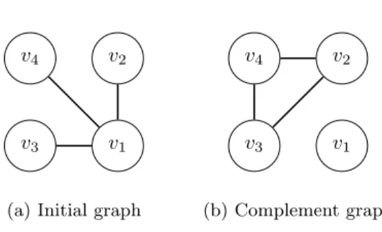
Example 2.2 Given a graph of 4 vertices and 3 edges as in Figure 1(a), the so-lution of the MaxClique problem is a clique of size 2. If we encode it as MaxOnes,
v1 v2
v3 v4
(a) Initial graph
v1 v2
v3 v4
(b) Complement graph
Figure 1: Graph in Example 2.2.
it is a CNF instance with binary clauses(¬x2∨ ¬x3),(¬x3∨ ¬x4),(¬x2∨ ¬x4).
Encoded as a Partial MaxSAT (MinSAT) instance is the same three binary hard clauses, and 4 positive (negative) unit soft clauses. Figure 1(b) shows the com-plement (or inverse) graph, with the same vertices than the previous graph such that two vertices are adjacent if and only if they are not adjacent in the ini-tial graph. This is the actual graph created by MinSatz estimation computation, since it finds a conflict between every two unit soft clauses with no edges in the initial graph.
Observe that this encoding produces a set of conflict implication chains
x1, x1 → ¬x2, x2, which consists of three clauses in Partial MaxSAT, two soft
unit clauses and one hard binary clause: {(x1),(x2),(¬x1∨ ¬x2)}. The same
implication is found in Partial MinSAT, but it consists of unit clauses having negative polarity.
In order to understand the behaviour of the two solvers, the following propo-sitions state how the two solvers perform when solving the two extreme cases of the MaxClique problem. At one extreme, when the graph is complete; at the other extreme, when the graph is empty.
Proposition 2.1 Given a MaxSAT or MinSAT encoding of the MaxClique
problem for the complete graph, there are no hard clauses.
Proposition 2.1 implies that both solvers easily solve the problem applying the pure literal rule, without searching.
Proposition 2.2 Given a Partial MaxSAT or Partial MinSAT encoding of the
MaxClique problem for the empty graph withnnodes, there arec=n·(n−1)/2
hard binary clauses. The behaviour of both solvers is the following: the upper
bound that MinSatz computes is 1 unsatisfied clause (i.e., n−1 satisfied soft
clauses); the lower bound that WMaxSatz computes is between n/2 and 3n/4
unsatisfied clauses, depending on the variable selection in the lower bound.
Solver MinSatz, for computing its upper bound in Proposition 2.2, performs the following steps: creates a graph withnvertices, which is a complete graph because it finds a conflict for every pair of soft clauses. Then, it runs the greedy
clique partition algorithm, which finds one clique with all the vertices, i.e.,n−1 satisfied clauses. This upper bound is actually the optimal solution.
Solver WMaxSatz, for computing its lower bound at the root node in Propo-sition 2.2, applies the lower boundU PF L∗ [16]. The result of such lower bound depends on the unit clause propagation ordering. In the worst case, it will give
n/2 unsatisfied clauses, because every pair of soft unit clauses implies one un-satisfied clause, since there exists a hard binary clause with those two literals negated. In the best case, it will give 3n/4 unsatisfied clauses, because every four soft unit clauses can give three unsatisfied clauses.
The reason is as follows: consider the four first unit clauses in the formula are
{(x1),(x2),(x3),(x4)}. The solver starts propagating the soft unit clause (x1),
finds a conflict with the soft clause (x2) and the hard clause (¬x1∨¬x2), so after
applying inference Rule 4, the solver replaces the soft unit clauses{(x1),(x2)}
by {,(x1∨x2)}. Then, the solver propagates the soft unit clause (x3) and
finds a conflict with soft clause (x1∨x2), and the two hard clauses (¬x1∨ ¬x3)
and (¬x2∨ ¬x3), so after applying inference Rule 5, the solver replaces the
soft clauses{(x3),(x1∨x2)} by{,(x1∨x2∨x3),(¬x1∨ ¬x2∨ ¬x3)}. Next,
the solver propagates the soft unit clause (x4) and finds a conflict with soft
clause (x1∨x2∨x3) and the three hard clauses (¬x1∨ ¬x4), (¬x2∨ ¬x4), and
(¬x3∨ ¬x4). At this point, the solver cannot apply any of its inference rules,
given that in the implication graph there is a ternary clause. Summarizing the action of inference rules, the solver replaces the initial set of four unit soft clauses by the following set of soft clauses: {,,(x1∨x2∨x3),(¬x1∨ ¬x2∨ ¬x3)}.
As a whole, the lower bound has been incremented by three given the initial four unit soft clauses. This scheme can be repeated along for every set of four unit soft clauses, which gives a total number ofb3n/4cconflicts. No more lower bound computations will be triggered by WMaxSatz because there are no unit clauses and because there are not enough positive and negative occurrences of any variable (it needs 2 positive and 2 negative occurrences at least, as it is explained by Li et al. in 2006).
Propositions 2.1 and 2.2 help to observe that when solving instances equiva-lent to MaxClique instances (clauses with only negative literals), the more dense is the graph, the lesser clauses in the 2SAT-MaxOnes encoding, and the easier for the two solvers. At one extreme, a complete graph (no hard binary clauses) is trivially solved. At the other extreme, a graph with no edges (n·(n−1)/2 binary clauses) is also trivially solved by solver MinSatz, since it finds a clique of sizen.
2.2
Instances with negative and positive literals in the
clauses
We continue the solver analysis for the case of instances where literals can be both negative and positive. Since the computation of the bounds in both solvers, WMaxSatz and MinSatz, are based on unit clause propagation, one of the important points for the computation of a good bound is the creation of implication chains. As seen in Section 2.1, an implication chain only involves
one binary clause when clauses have only negative literals. In this section, we show that an implication chain can involve several binary clauses in the more general case (clauses with negative and positive literals).
Lemma 2.1 Any conflict vertex in a conflict implication graph of a 2SAT-MaxOnes instance can be derived only by one or two unit clauses in the input formula.
Prof 3 There are two kinds of conflict vertices:
1. The conflict vertex is associated with an input binary clause(li∨lj). Such
a conflict is reached with a pair of implication chains. The pair of implica-tion chains can have two different forms: (i) two independent implicaimplica-tion
chains starting with two different input unit clauses, one finishing with(¯li)
and the other one finishing with (¯lj); (ii) two implication chains starting
with one common input unit clause, one finishing with (¯li)and the other
one finishing with(¯lj).
2. The conflict vertex is associated with two input unit clauses(l1) and(li).
Such a conflict is reached with one implication chain starting with(l1)and
finishing with (¯li).
Given Lemma 2.1, we investigate two cases of conflicts in implication graphs that influence the estimation computation: a Two-Unit conflict, a conflict de-rived by two input unit clauses, and a One-Unit conflict, a conflict dede-rived by one input unit clause. We focus on conflicts generated where all the input unit clauses are positive in a Partial MaxSAT encoding, and negative in a MinSat encoding, since these are the polarities in a 2SAT-MaxOnes encoding.
ATwo-Unit conflict is a conflict implied by two input unit clauses:
x11, x11→x12→ · · · →x1m→x
x21, x21→x22→ · · · →x2n→ ¬x (1)
The two implication chains consist of the two soft unit clauses (x11) and (x21), and the following set of hard binary clauses:
(¬x11∨x12),(¬x21∨x13), . . . ,(¬x1m∨x)
(¬x2
1∨x22),(¬x22∨x23), . . . ,(¬x2n∨ ¬x)
(2)
When this set of clauses is in the formula, the two solvers compute the same bound value with different strategies.
Solver WMaxSatz . Let us assume WMaxSatz starts propagating unit clauses
(x1
1) and (x21), then it finds the implication chains in (1). It increments
following set of soft binary clauses, to preserve the set of solutions, by applying Rule 4 (cf. Section 2):
(x1
1∨ ¬x12),(x12∨ ¬x13), . . . ,(x1m∨ ¬x)
(x2
1∨ ¬x22),(x2∨ ¬x23), . . . ,(x2n∨x)
(3)
Then, it propagates soft unit clauses (x1
2) and (x22), finds a conflict,
re-moves the two unit clauses, and adds the following set of soft binary clauses:
(x1
2∨ ¬x13), . . . ,(x1m∨ ¬x)
(x2
2∨ ¬x23), . . . ,(x2n∨x)
The process is repeated k times, where k= min(m, n). At the end, the solver has found k conflicts. Observe that for any other order of propa-gation for the first k pairs of soft unit clauses, with pairs with one unit clause in the first chain and the other in the second chain, the computed bound is the same.
Solver MinSatz negates every pair of unit soft clauses and checks if there exists a conflict. Let us assume it starts with the pair of unit clauses (¬x1
1) and (¬x12). The solver does not detect any conflict. The same
happens with any pair of unit clauses in the same implication chain. Let us assume it continues with the pair (¬x1
1) and (¬x21). The solver does
detect a conflict. The same happens with any pair of unit clauses with every clause from a different chain, i.e., unit clause (¬x1
1) conflicts with
unit clauses (¬x2
1), . . . ,(¬x2n); unit clause (¬x12) conflicts with unit clauses
(¬x21), . . . ,(¬x2n), and so on for all the unit clauses in the first chain. The solver creates a graph with nodes corresponding to unit clauses, and an edge between every pair with the first unit clause in the first chain and the second unit clause in the second chain. Additionally, edges between all nodes in the first chain and nodexare created, since every unit clause in such a chain conflicts with x. At this point, a bipartite graphKm,n+1
has been created. The solver is going to partition the graph into cliques to compute the bound. The clique partition greedy algorithm selects the vertex with larger degree, and selects one clique of size 2, the maximum size. Then, it removes its vertices from the graph, and selects another vertex with maximum degree, and so on. At the end, the algorithm has selectedk= min(m, n) cliques of size 2. The upper bound is incremented byk. Then, a Partial MaxSAT formula is created withm×(n+ 1) hard clauses (¬x1
i∨ ¬x2j), one for every edge, and withksoft clauses (x1i∨x2j),
one for every clique, which bring no more conflicts.
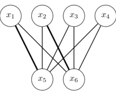
Example 2.3 Let be a 2SAT-MaxOnes instance with 6 variablesx1, . . . , x6 and
the following set of clauses:
(¬x1∨x2),(¬x2∨x3),(¬x3∨x4),(¬x4∨ ¬x5),(x5∨ ¬x6). (4)
The correspondence of variables in this example and variables in (1) is the fol-lowing: x1=x11, x2=x12, x3=x31, x4=x, x5=x21, x6=x22.
x1 x2 x3 x4
x5 x6
Figure 2: MinSAT graph for Example 2.
The MaxSAT encoding hardens the clauses in (4) and adds the soft unit clauses: (x1),(x2),(x3),(x4),(x5),(x6). Solver WMaxSatz finds 2 unsatisfied
clauses. Assuming the unit pairs are(x1, x5),(x2, x6), the solver adds the
fol-lowing soft binary clauses for the first pair: (x1∨¬x2),(x2∨¬x3),(x3∨¬x4),(x4∨
x5), and the following soft binary clauses for the second pair: (x2∨ ¬x3),(x3∨
¬x4),(x4∨x5),(¬x5∨x6).
The MinSat encoding also hardens the clauses in (4) and adds the soft unit clauses(¬x1),(¬x2),(¬x3),(¬x4),(¬x5),(¬x6). Sincem= 3 andn= 2, solver
MinSatz finds 2 unsatisfied clauses. Then, it creates a Partial MaxSAT formula with one hard clause for every edge in the graph: (¬x1∨¬x5),(¬x1∨¬x6),(¬x2∨
¬x5),(¬x2∨ ¬x6),(¬x3∨ ¬x5),(¬x3∨ ¬x6),(¬x4∨ ¬x5),(¬x4∨ ¬x6). And
finally, it adds one soft binary clause for every clique in the graph. Assuming the solver has found the cliques (x1, x5),(x2, x6), then it adds the soft binary
clauses: (x1∨x5),(x2∨x6) to the formula. Figure 2 represents the MinSAT
graph for this example.
A second structure deriving a conflict found in 2SAT-MaxOnes instances is the One-Unit conflict. AOne-Unit conflict is a conflict implied by two im-plication chains starting with a common sequence (prefix), and ending with complementary literals:
x1, x1→ · · · →xp→x11→x12→ · · · →x1m→ ¬x
x1, x1→ · · · →xp→x12→x22→ · · · →x2n→x.
Such two implication chains consist of one soft unit clause (x1) and the following
set of hard binary clauses:
(¬x1∨x2),(¬x2∨x3),· · ·,(¬xp−1∨xp),
(¬xp∨x11),(¬x11∨x12),· · ·,(¬x1m∨ ¬x),
(¬xp∨x21),(¬x21∨x22),· · ·,(¬x2n∨x).
(5)
In the following, we split the two implication chains in three sequences of clauses: the prefix (the first raw in (5)), the first sequence (the second raw in (5)), and the second sequence (the third raw in (5)).
Solver WMaxSatz . Let us assume WMaxSatz starts propagating the unit soft clause (x1), then it finds a conflict involving such a soft clause and
the binary hard clauses in (5). It increments the lower bound by one, removes such a soft clause and adds a set of soft clauses by applying inference rules (e.g. Rule 5). Then, it propagates unit clause (x2), finds
a conflict, increments the lower bound by one, removes such a soft clause and adds a set of soft clauses. An so on until unit soft clause (xp). Then,
it propagates (x1
1), finds a conflict with clause (x), and removes both unit
clauses. Then, it propagates (x1
2), finds a conflict with clause (x2n), and
removes both unit clauses. And so onktimes, wherek= min(m, n+ 1). At the end, WMaxSatz finds p+k conflicts. Observe that for any other order of soft unit clauses, the computed bound is the same.
Solver MinSat negates every pair of unit soft clauses and checks if a conflict is derived. The solver does not detect a conflict if the two clauses in the pair are in the same sequence. The solver, instead, does detect a conflict if the two clauses are in different sequences. For example, if unit clauses (¬x1)
and (¬x11) are negated and propated, a conflict is found. All unit clauses
in the prefix sequence conflict with all unit clauses in the first and second sequences. And all unit clauses in the first sequence conflict with all unit clauses in the second sequence. Observe that a tripartite graphKm,n+1,p
has been created. The greedy partition algorithm selects one vertex with maximum degree, in this case 3, and it finds a clique of maximum size, in this case 3. Because this is a tripartite graph, there will be min(p, m, n+1) cliques of size 3. Assume w.l.o.g. thatp≤n+ 1≤m. Then, the number of cliques of size 3 isp, and the number of cliques of size 2, after removing edges of cliques of size 3, is (n+ 1)−p. The total number of cliques found isp+ ((n+ 1)−p) =n+ 1. At the end, MinSat findsn+ 1 conflicts.
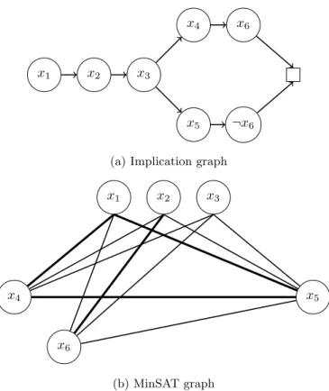
Example 2.4 Let be a 2SAT-MaxOnes instance with 6 variablesx1, . . . , x6 and
the following set of clauses:
(¬x1∨x2),(¬x2∨x3),(¬x3∨x4),(¬x4∨ ¬x6),(¬x3∨x5),(¬x5∨x6). (6)
The correspondence of variables in this example with variables in (5) is the following: x1=x1, x2=x2, x3=xp, x4=x11, x5=x21, x6=xn.
The MaxSAT encoding hardens the clauses in (6) and adds the soft unit clauses: (x1),(x2),(x3),(x4),(x5),(x6). Assuming a lexicographic order of
prop-agation, solver WMaxSatz starts propagating (x1)and finds a conflict with the
set of hard binary clauses. It removes such unit clause and adds a set of soft
binary clauses. Then, it propagates (x2), finds a conflict with the set of hard
binary clauses, removes such a unit clause and adds a set of soft binary clauses.
Then, it propagates(x3), finds a conflict, removes such a unit clause, and adds
a set of soft binary clauses. Then, it propagates(x4), finds a conflict with the
soft unit clause(x5), removes such unit clauses and adds the set of soft binary
x1 x2 x3
x4
x5
x6
¬x6
(a) Implication graph
x1 x2 x3
x4 x5
x6
(b) MinSAT graph
Figure 3: Implication graph and MinSAT graph for Example 2.4.
Solver WMaxSatz has found 4 unsatisfied clauses. The MaxSatz implication graph is displayed in Figure 3 (a).
The MinSAT encoding hardens the clauses in (6) and adds the soft unit clauses: (¬x1),(¬x2),(¬x3),(¬x4),(¬x5),(¬x6). Solver MinSatz creates a graph
with 6 nodes and 16 edges, displayed in Figure 3 (b). The partition algorithm
selects the vertex with maximum degree, i.e. x5with degree 5. Assuming a
lexi-cographic order, it detects one clique of size 3 involving nodesx1, x4, x5. Then,
it selects the vertex with maximum degree, i.e. x6 with degree 4. Assuming
also a lexicographic order, it detects one clique of size 2 involving nodes x2, x6.
Solver MinSatz has found 2 unsatisfied clauses.
Apart from detecting the larger number of conflicts, the application of infer-ence rules helps to speed up the solver. WMaxSatz applies inferinfer-ence rules after each conflict found, whilst in the version of MinSatz used, such a formula trans-formation has not been implemented. As explained by Li et al. [17], adding more clauses thanks to inference rules may help finding more conflicts by estimations.
Note that the number of occurrences of positive and negative literals for almost every variable in a Two-Unit conflict and in a One-Unit conflict is exactly the same. Such a set of clauses could be generated in Random 2SAT-MaxOnes instances whenp= 0.5. Increasing or decreasingp, the same structure may still appear, but probably with a shorter length. So, we next consider the study of the complexity of solving typical instances of Random-p2SAT-MaxOnes.
3
Satisfiability Phase Transition for Random-
p
2SAT-MaxOnes
In the previous section the analysis we have performed on some particular cases of 2SAT-MaxOnes instances has shown that the fraction of positive literals on the clauses can have an impact on the bounds computed by both algorithms, given that the possible structures in the instances depend, among other char-acteristics, on the fraction of positive literals. So, the next step is to study to what extent the solving performance of both solvers is affected by the fraction of positive literals in large sets of instances. To this end, we propose to study the typical case complexity of Random-p2SAT-MaxOnes, where instances are generated by uniformly at random selecting the variables in the clauses, but the polarity of any literal is selected as positive with probabilitypand negative with probability (1−p). Given that for 0< p <1 Random-p2SAT-MaxOnes may give unfeasible instances, observe that whenp= 0.5 the set of clauses follows the same distribution as on the classical Random 2SAT problem, we want to study, and predict as much as possible, the location of the phase transition from feasi-ble to unfeasifeasi-ble instances as the ratioc/nincreases. Observe that an unfeasible Random-p2SAT-MaxOnes instance may be solved in polynomial time, so it is clear that if we are interested in studying the hardest instances, they should be found always on the feasible region, so bounding the feasible region will help to locate the hardest instances. So, in this section we first study the satisfiability (feasibility) phase transition for Random-p2SAT-MaxOnes and then in the next section we study its typical complexity and its possible relation with the bounds computed by both algorithms as we have studied in Section 2. The satisfiabil-ity phase transition for Random-p2SAT-MaxOnes is determined by the set of binary clauses contained in the instances. So, we denote as Random-p2SAT a Random 2SAT problem where the polarity of each literal is chosen positive with probabilitypand negative with probability (1−p).
The phase transition for Random 2SAT was analyzed in by Goerdt in [12], where it was shown that there is a sharp phase transition when nc = 1. The analysis is based on the study of the number of cycles in normal form when
c
n <1 and on the study of the number of simple cycles when c
n >1. See [12] for
the formal definition of these kinds of cycles in the formula graph. In our case, we study an upper bound on the location of the phase transition by analyzing the mean number of simple cycles in a Random-p2SAT instance.
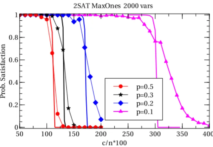
p=0.5 p=0.3 p=0.2 p=0.1 2SAT MaxOnes 2000 vars
Pr ob . S at is fa ct io n 0 0.2 0.4 0.6 0.8 1 c/n*100 50 100 150 200 250 300 350 400
Figure 4: Empirical (solid line with points) and lower bound computation (solid line) on satisfiability phase transition for Random-p2SAT instances with 2000 variables
O (c/n)l
. A simple cycle has only a complementary pair of literals, let’s say
xand¬xand the path from xto ¬xconsists of v=l/2−1 literals (excluding
xand ¬x), as many as the reverse path, containing both paths of literals no complementary pairs. That is, a simple cycle of lengthl = 2v+ 2 can be seen as the union of these two simple paths:
x→l1→. . .→lv → ¬x (7) ¬x→g1→. . .→gv →x (8)
where (x,¬x) is the only complementary pair of literals among the literals in the cycle.
Such calculations can be extended for Random-p2SAT problems considering that any simple cycle of lengthl, when expressed as 2SAT clauses, has exactlyl
clauses, withlpositive literals andl negative literals. Now, we have to consider the generation model. In our case, we pickc pairs of different variables among
N = n2
at random and we negate each variable with probability 1−p. Then, from the set of possible sets ofcpairs of variables ( Nc), we have that only Nc−−ll contain a given set oflpairs of variables. Finally, there arelpositive literals and
l negative literals in all thel clauses of the cycle, so the right polarity for the literals is obtained with probabilitypl(1−p)l. So, the probability of obtaining a given simple cycle (π) of lengthl is
Pπl =pl(1−p)l N−l c−l N c .
Considering that a simple cycle of length l is composed withl−2 literals (v = l/2−1 literals in the first and in the second path) and a selected pair
of complementary literals (x,¬x), we can obtain the number of distinct simple cycles of lengthl considering the following sequence of choices: (i) Select the complementary pair (n possibilities) (ii) From the remaining n−1 variables, select thev=l/2−1 remaining variables of the first simple path, order them, and select their polarity. Because this model generates a same simple path in two equivalent forms, the total number of distinct simple paths with thev
variables is n−v1
·v!·2v−1 (iii) For the second simple path, it only remains to
select its set ofvliterals with a choosen polarity, exactly like in the first simple path, but now the number of variables to choose from is n−1−v. So, the number of simple cycles of lengthl is:
µl=n· n −1 v ·v!·2v−1· n −1−v v ·v!·2v−1 and compute the expected number of simple cycles,X, as
E[X] =X
l
µl·Pπl.
In [12] Goerdt showed that almost always a Random-0.5 2SAT unsatisfi-able instance contains a simple cycle of logarithmic length (with respect to the number of variablesn). So, if we assume that for the general Random-p2SAT problem still is enough to focus on simple cycles1for asymptotically determin-ing unsatisfiable instances, the unsatisfiability probability for an instance can be upper bounded by Markov’s inequality over the random variableX:
P r(U nsat) =P(X≥1)≤E[X] (9) Figure 4 shows the curves for the phase transition, the value P r(Sat), em-pirically obtained from experiments with test sets of instances with n= 2000 and with different values of p and c/n with 300 instances per each c/n ratio and value of p. It also shows the curves for the approximation of the phase transition obtained from Equation (9) for the same sets of instances. That is, it shows the value
1−min(1, E[X])
Observe that given thatmin(1, E[X]) is an upper bound on the unsatisfiability probability, 1−min(1, E[X]) is a lower bound on the satisfiability probability. The value we actually compute for E[X] considers as range of values for the cycle lengths the range [1,75], that is enough for capturing cycles of logarithmic length with respect to the value of n (2000) in these test sets. It is worth noticing that the lower bound on the satisfiability phase transition is very close to the real one, although the prediction is better for values ofpnear to 0.5.
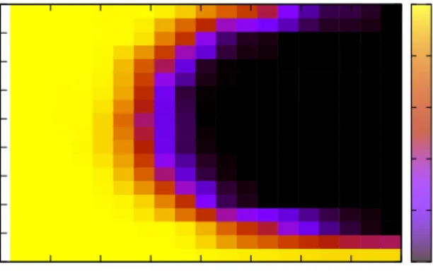
Figure 5 shows the curves for the phase transition obtained from experiments withn=100, and with values forpfrom 0.0 to 0.9. Observe that the curves are symmetric around the valuep= 0.5, because the satisfiability of a set of 2SAT clauses does not change if we rename positive literals to negative ones, and negative literals to positive ones.
100 vars. 0 50 100 150 200 250 300 350 400 c/n * 100 0 10 20 30 40 50 60 70 80 90 p * 100 0 0.2 0.4 0.6 0.8 1 Prob. Satisfaction
Figure 5: Phase transition for Random-p2SAT-MaxOnes
4
Typical Case Complexity for Random-
p
2SAT-MaxOnes
In Section 2 we analyzed how the presence of certain structures, with different fractions of positive literals, affects the bounds computed by both algorithms. Then, in Section 3 we analyzed the satisfiability phase transition for Random-p
2SAT-MaxOnes in order to locate the hardest instances of the problem. Next, in this section we investigate the typical case complexity of Random-p 2SAT-MaxOnes. Our aim is to compare the solvers performance either in cases with no positive literals (p= 0) or in cases with positive literals (p >0), so we can study instances that can contain the structures studied in Subsection 2.1 and in Subsection 2.2 and check whether the behaviour analyzed in these particular instances allows to understand the behaviour for wider sets of instances.
4.1
Typical Case Complexity for
p
= 0
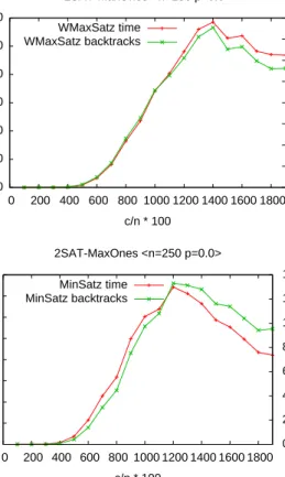
We start our study of typical case complexity with Random-0 2SAT-MaxOnes instances, solving them with WMaxSatz and MinSatz. Figure 6 shows the results obtained when solving test sets with 250 variables, where the horizontal axis shows the c/n ratio of each test set of 100 instances. We show both the median time and the median number of backtracks performed in the search tree for solving the instances. We observe an easy-hard-easy pattern in the hardness of the instances, with the hardest instances located around the ratio 13 in the case of WMaxSatz and around 12 in the case of MinSatz. But observe that the decrease in typical complexity seems more abrupt for MinSatz than for
0 500 1000 1500 2000 2500 3000 0 200 400 600 800 1000 1200 1400 1600 1800 0 1e+06 2e+06 3e+06 4e+06 5e+06 6e+06 7e+06 8e+06
Median CPU time in seconds Median number of backtracks
c/n * 100 2SAT-MaxOnes <n=250 p=0.0> WMaxSatz time WMaxSatz backtracks 0 50 100 150 200 250 300 350 400 0 200 400 600 800 1000 1200 1400 1600 1800 0 200000 400000 600000 800000 1e+06 1.2e+06 1.4e+06
Median CPU time in seconds Median number of backtracks
c/n * 100
2SAT-MaxOnes <n=250 p=0.0> MinSatz time
MinSatz backtracks
Figure 6: Typical case complexity of Random-0 2SAT-MaxOnes with WMaxSatz and MinSatz.
WMaxSatz.
The results indicate a clear advantage of MinSatz with respect to WMaxSatz, in the whole range ofc/n ratios tested, not only on the solving time, but also in the size of the search tree, meaning that the advantage of MinSatz is mainly to a better pruning of the search space when looking for the optimal solution. Remember that the behaviour of both solvers, with respect to their computed bounds, analyzed in Proposition 2.2, indicated an advantage of MinSatz in the extreme case where the instance, with only negative literals, contains all the possible binary clauses. In that case, the upper bound computed by MinSatz was equal to the optimum solution. But our empirical results indicate that MinSatz has a advantage over WMaxSatz over a wider set ofc/nratios.
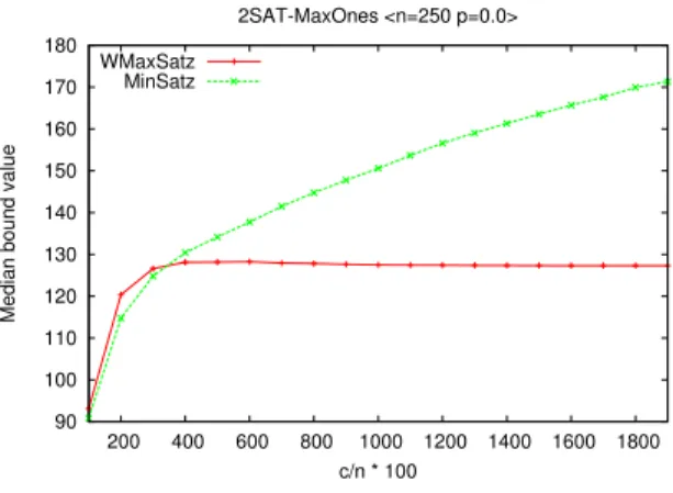
To check whether the advantage of MinSatz with respect to WMaxSatz can also be related to the difference in their computed bound for all thec/n ratios tested, and not just in the highest one, we have empirically investigated the bounds computed by both algorithms at the root node of their search tree. In Figure 7 we can see the median value of the bound computed in the root node for the same set of instances as before.2 We observe that WMaxSatz lower bound improves as the ratio is increased, but it stabilizes aroundn/2 forc/n≥
3. As we have seen in Proposition 2.2, this is the worst case for WMaxSatz, when it consumes the highest possible number of original unit clauses to detect conflicts. So, well before reaching the extreme case analyzed in Proposition 2.2, WMaxSatz is obtaining the worst possible lower bound. In contrast, MinSatz gives a monotone increment in its bound value. That probably means the clique partition based upper bound is discovering bigger cliques when the ratio c/n
is increasing, tending to the best possible value, which happens when all the vertices are in one clique.
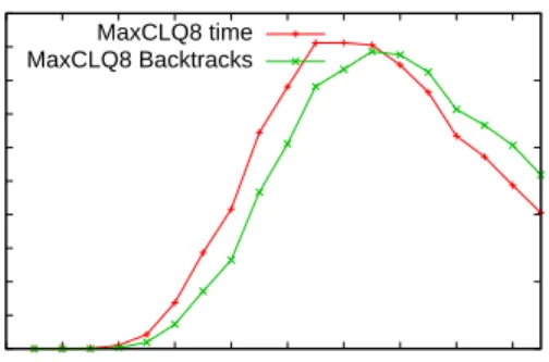
Given that Random-0 2SAT MaxOnes instances are equivalent to MaxClique instances (cf. Proposition 1.1), we have also solved these sets of instances with an state-of-the-art MaxClique solver to check whether a similar behaviour is ob-served when the instances are rewritten and solved as MaxClique instances. We have chosen the solver MaxCLQ [18], that has shown an excellent performance compared with previous MaxClique solvers. MaxCLQ is a branch and bound solver, with similar algorithm and data structures to the ones of WMaxSatz and MinSatz and with an upper bound computed by finding a clique partition as in MinSatz, which is improved with an encoding of the partition into Partial MaxSAT and solved using MaxSAT technology.
Figure 8 shows the median time to solve Random-0 2SAT MaxOnes instances with MaxCLQ when the instances are transformed to MaxClique instances. This time the hardness peak for MaxCLQ is located around the ratio c/n = 10, but overall the complexity pattern is similar to the one of WMaxSatz and MinSatz. Observe that the descending slope to the right of the hardness peak
2As commented in Section 2, the number of positive variables in an assignment for a
MaxOnes instance is equal to the number of satisfied soft clauses in the Partial MaxSAT encoding and equal to the number of unsatisfied soft clauses in the Partial MinSatz encoding. So, in the figure we compare the number of unsatisfied clauses given by the lower bound of WMaxSatz with the numbern−k, wherekis the upper bound given by MinSatz.
90 100 110 120 130 140 150 160 170 180 200 400 600 800 1000 1200 1400 1600 1800
Median bound value
c/n * 100 2SAT-MaxOnes <n=250 p=0.0> WMaxSatz
MinSatz
Figure 7: Median value of the bounds computed by WMaxSatz and MinSatz at the root node.
is steeper for MaxCLQ, gentle for WMaxSatz, and in the middle for MinSatz. The reason for the steeper descend of MaxCLQ with respect to MinSatz could be that MaxCLQ takes advantage of additional speedups obtained thanks to the MaxClique specialized internal representation of the problem.
Table 1 shows the median solving time for instances at the ratio 10.0 obtained with the three solvers. The results show that for such a ratio the hardness of the instances increases exponentially. Actually, the relative increase seems to be very similar for the three solvers: for every increase of 10 variables the time is doubled. However, in absolute figures, MaxCLQ and MinSatz are always better than WMaxSatz. Analyzing the median number of backtracks and median time for each solver we observe that the number of backtracks per second is very similar for solvers WMaxSatz and MinSatz as the problem size increases. So, that means the advantage of MinSatz with respect to WMaxSatz is mainly due to having a smaller search tree. Observe also that the number of backtracks for MaxCLQ at least doubles the number of backtracks for the other solvers, even though its time is smaller. The reason probably could be the data structures and the techniques used in MaxCLQ are optimized for such a problem. Observe that the time results are consistent with the experimentation performed with analogue MaxClique instances in [19].
The good performance of MaxCLQ indicates that, even if the three solvers are branch-and-bound based solvers, there is some place for improvement of the WMaxSatz and MinSatz solvers on 2SAT-MaxOnes instances when the clauses have only negative literals, at least for the random instances tested here.
4.2
Typical Case Complexity for
p >
0
Whenp >0, a phase transition from feasible to unfeasible instances appears, as we have analyzed in Section 3. The hardest instances are located in the feasible
0 10 20 30 40 50 60 70 80 90 100 0 200 400 600 800 1000 1200 1400 1600 1800 0 500000 1e+06 1.5e+06 2e+06 2.5e+06
Median CPU time in seconds Median number of backtracks
c/n * 100
2SAT-MaxOnes <n=250 p=0.0> MaxCLQ8 time
MaxCLQ8 Backtracks
Figure 8: Performance of MaxCLQ on Random-0 2SAT MaxOnes instances as MaxClique instances.
Table 1: Complexity scaling for MaxCLQ, MinSatz and WMaxSatz at thec/n
ratio 10.0 andp= 0.0, in time and backtracks
vars. MaxCLQ MinSatz WMaxSatz
secs bkts bkts/sec secs bkts bkts/sec secs bkts bkts/sec 220 12 285309 23775.75 50 177073 3541.46 219 753466 3440.48 230 22 532686 24213.00 85 282778 3326.80 389 1255415 3227.28 240 38 997316 26245.15 174 553693 3182.14 778 2388147 3069.59 250 77 1647659 21398.16 304 882601 2903.29 1429 4120595 2883.55 260 150 2938649 19590.99 555 1536242 2768.00 2803 7804625 2784.38
region, just to left of the phase transition, and then the hardness decreases before reaching the region with 100% unfeasible instances. This was observed before by Slaney and Walsh for the problems Random-12 2SAT-MaxOnes and Random-12 3SAT-MaxOnes [25].
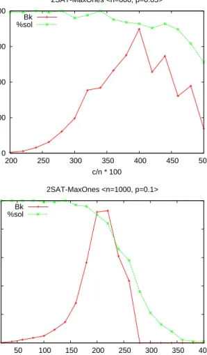
Beyond the existence of the feasible-unfeasible phase transition, two inter-esting properties of the problem change as we increase p. First, the typical hardness of the instances decreases aspincreases, and the hardest instances are found concentrated in a narrower region. Figure 9 shows the median number of backtracks (red plot), and percentage of feasible instances (green plot) for instances withp= 0.05 and n= 600 (top) and for instances with p= 0.1 and
n = 1000 (bottom). We show results for instances with such high number of variables, because for smaller number of variables the values obtained are not as significant as the ones obtained withp= 0.0.
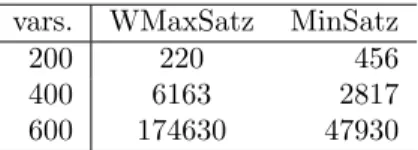
The second property that changes, aspincreases, is the relative performance of both solvers. We have studied the solving cost scaling of WMaxSatz and MinSatz whenp= 0.05 and p= 0.1 forc/n= 4.0 andc/n= 2.2, respectively. The results are shown in Tables 2 and 3. Times are not shown since they are lower than 1 second. For p = 0.05, as n is increased, MinSatz is still better than WMaxSatz, although now the difference is only about 3 times better, in contrast to the case p = 0.0 where MinSatz was about 5 times better. For
p= 0.1, the behaviour changes completely, as now WMaxSatz is better: about 13 times better. Even if the hardness for p = 0.1 has decreased down to a point where its complexity scaling seems to be almost linear, observe that in the worst case Random-p2SAT-MaxOnes for p <1 will provide exponentially hard instances (Corollary 1.1).
Table 2: Complexity scaling for MinSatz and WMaxSatz at c/n = 4.0 and
p= 0.05, in backtracks
vars. WMaxSatz MinSatz 200 220 456 400 6163 2817 600 174630 47930
Remember that in Subsection 2.2 we analyzed instances, with structures that contained positive literals in the clauses, where WMaxSatz could be more powerful than MinSatz (the One-Unit conflict structures), due to the better quality of the lower bound obtained by WMaxSatz in these instances. The fraction of positive literals in those structures was 0.5, but of course in
Random-p2SAT MaxOnes instances they can be present whenpis any value greater than 0, although these structures will be more frequent and larger whenpapproaches to 0.5. To check whether the advantage of WMaxSatz with respect to MinSatz aspincreases can be related to the bound computed by the algorithms, we have computed the median value of the bounds computed by both algorithms at the
0 50000 100000 150000 200000 200 250 300 350 400 450 500 Median Backtracks %sat instances
c/n * 100 2SAT-MaxOnes <n=600, p=0.05> Bk %sol 0 200 400 600 800 1000 50 100 150 200 250 300 350 400 Median Backtracks %sat instances
c/n * 100
2SAT-MaxOnes <n=1000, p=0.1> Bk
%sol
Figure 9: Typical case complexity for Random-0.05 2SAT-MaxOnes with 600 variables and Random-0.1 2SAT-MaxOnes with 1000 variables with solver WMaxSatz.
Table 3: Complexity scaling for MinSatz and WMaxSatz at c/n = 2.2 and
p= 0.1, in backtracks
vars. WMaxSatz MinSatz 600 215 3894 800 364 7192 1000 930 11566 1200 1190 17180 0 20 40 60 80 100 120 50 100 150 200 250 300 350 400
Median bound value
c/n * 100
2SAT-MaxOnes <n=200, p=0.05> MinSatz
WMaxSatz
Figure 10: Median value of the bounds computed by WMaxSatz and MinSatz forp= 0.05 at the root node.
root node of the search tree. In Figures 10 and 11 we can see the median value of the number of unsatisfied clauses bound computed in the root node for the same set of instances as before. We observe that forp= 0.05, where MinSatz is still better than WMaxSatz although with a difference not as big as forp= 0.0, the bounds are very close with a slight advantage of WMaxSatz with respect to MinSatz, so this can explain in part why now MinSatz is not as good as for p = 0.0. For p = 0.1, we observe that the advantage of WMaxSatz with respect to MinSatz increases more as the ratio increases, so this could explain in part why now the relative behaviour of both solvers changes: now WMaxSatz is better than MinSatz. This could be due to the presence of more One-Unit conflict structures, like the ones explained in Example 2.4, where WMaxSatz is able to obtain better bounds than MinSatz. Although we only show results for the bound computed in the root node, this bound is computed at each node of the search tree, and probably the improvement at each node is small, but
0 20 40 60 80 100 50 100 150 200
Median bound value
c/n * 100
2SAT-MaxOnes <n=200, p=0.1> MinSatz
WMaxSatz
Figure 11: Median value of the bounds computed by WMaxSatz and MinSatz forp= 0.1 at the root node.
the global improvement could be enough to explain the overall performance difference between both solvers.
5
Conclusions and further work
In this work we have performed an analysis of the behaviour of two well known branch and bound algorithms: WMaxSatz and MinSatz when solving 2SAT-MaxOnes instances, either particular instances with certain structures present or sets of instances from Random-p2SAT-MaxOnes.
The analysis on the particular instances has allowed us to undercover sig-nificant differences in the quality of their computed bounds depending on the presence of certain structures that may or not may be present depending, among other factors, on the number of positive literals on the clauses. Then, an em-pirical analysis of typical instances from Random-p2SAT-MaxOnes has shown that the performance difference between both solvers when solving wider sets of 2SAT-MaxOnes instances can also be related to their difference in the quality of their computed bound and that this difference can also be related to the fraction of positive literals, controlled with the parameterp. We think that our results can help develop more efficient and robust solvers for 2SAT-MaxOnes. On the one hand, we think that the success of WMaxSatz whenp >0 indicates that the use of inference rules can make a difference when computing the bounds on these instances. On the other hand, for the case of instances with no positive literals the upper bound computed thanks to the MinSAT graph is better than the lower bound computed by WMaxSatz. So, some kind of combination of
both techniques could be considered for obtaining a more robust, and possibly more efficient, solver for 2SAT-MaxOnes.
In the near future we plan to investigate the behaviour of another class of algorithms for solving optimization problems that is proving very successful for industrial applications of Partial MaxSAT: the unsatisfiable cores based algo-rithms (see [23] for an extended survey of such algoalgo-rithms). In addition, we also plan to study the relevance of the results of this paper with industrial MaxSAT instances that can share similar structures that the ones analized here, but they may also have other relevant features for the solvers performance.
References
[1] A. Abram´e and D. Habet. On the resiliency of unit propagation to max-resolution. In Proceedings of the 24th International Joint Conference on
Artificial Intelligence, 2015.
[2] C. Ans´otegui, M. L. Bonet, and J. Levy. Solving (weighted) partial MaxSAT through satisfiability testing. In Proc. of SAT 2009, pages 427– 440, 2009.
[3] C. Ans´otegui, M. L. Bonet, and J. Levy. Sat-based maxsat algorithms.
Artif. Intell., 196:77–105, 2013.
[4] J. Argelich, R. B´ejar, C. Fern´andez, and C. Mateu. On 2sat-maxones with unbalanced polarity: from easy problems to hard maxclique problems. In
Proceedings of CCIA’2011, volume 232 ofFrontiers in Artificial Intelligence
and Applications, pages 21–30. IOS Press, 2011.
[5] J. Argelich, C. M. Li, F. Many`a, and J. Planes. The first and second MaxSAT evaluations. JSAT, 4(2–4):251–278, 2008.
[6] J. Argelich, I. Lynce, and J. P. Marques-Silva. On solving boolean multilevel optimization problems. InProc. of IJCAI 2009, pages 393–398, 2009. [7] A. Biere, M. Heule, H. van Maaren, and T. Walsh, editors. Handbook of
Satisfiability, chapter Conflict-Driven Clause Learning SAT Solvers. IOS
Press, 2009.
[8] N. Bjorner and N. Narodytska. Maximum satisfiability using cores and correction sets. In Proceedings of the 24th International Joint Conference
on Artificial Intelligence, 2015.
[9] B. Cha, K. Iwama, Y. Kambayashi, and S. Miyazaki. Local search algo-rithms for partial MaxSAT. InAAAI’97, pages 263–268, 1997.
[10] Y. Chen, S. Safarpour, A. G. Veneris, and J. P. Marques-Silva. Spatial and temporal design debug using partial MaxSAT. InProc. of 19th ACM Great
[11] J. Conrad, C. P. Gomes, W. J. van Hoeve, A. Sabharwal, and J. Suter. Connections in networks: Hardness of feasibility versus optimality. InProc.
of CPAIOR2007, pages 16–28, 2007.
[12] A. Goerdt. A threshold for unsatisfiability. J. Comput. Syst. Sci., 53(3):469–486, 2006.
[13] A. Gra¸ca, I. Lynce, J. Marques-Silva, and A. L. Oliveira. Haplotype in-ference combining pedigrees and unrelated individuals. In WCB09, pages 27–36, September 2009.
[14] J. H˚astad. Clique is hard to approximate withinn(1−). InFOCS’06, pages
627–636, 1996.
[15] C. M. Li and F. Many`a. An exact inference scheme for minsat. In
Proceed-ings of the 24th International Joint Conference on Artificial Intelligence,
2015.
[16] C. M. Li, F. Many`a, N. O. Mohamedou, and J. Planes. Resolution-based lower bounds in MaxSAT. Constraints, 15(4):456–484, 2010.
[17] C. M. Li, F. Many`a, and J. Planes. New inference rules for Max-SAT. J.
Artif. Intell. Res. (JAIR), 30:321–359, 2007.
[18] C. M. Li and Z. Quan. An efficient branch-and-bound algorithm based on MaxSAT for the maximum clique problem. In Proceedings of AAAI’10, pages 128–133, 2010.
[19] C. M. Li, Z. Zhu, F. Many`a, and L. Simon. Optimizing with minimum satisfiability. Artificial Intelligence, 190:32–44, 2012.
[20] J. Marques-Silva, J. Argelich, A. Gra¸ca, and I. Lynce. Boolean lexico-graphic optimization: algorithms & applications. Ann. Math. Artif. Intell., 62(3-4):317–343, 2011.
[21] R. Martins, V. M. Manquinho, and I. Lynce. Open-WBO: A modular maxsat solver,. In Theory and Applications of Satisfiability Testing - SAT 2014 - 17th International Conference, Held as Part of the Vienna Summer
of Logic, VSL 2014, Vienna, Austria, July 14-17, 2014. Proceedings, pages
438–445, 2014.
[22] A. Morgado, C. Dodaro, and J. Marques-Silva. Core-guided maxsat with soft cardinality constraints. In Principles and Practice of Constraint Programming - 20th International Conference, CP 2014, Lyon, France,
September 8-12, 2014. Proceedings, pages 564–573, 2014.
[23] A. Morgado, F. Heras, M. H. Liffiton, J. Planes, and J. Marques-Silva. It-erative and core-guided MaxSAT solving: A survey and assessment.
[24] E. D. Rosa, E. Giunchiglia, and M. Maratea. Solving satisfiability problems with preferences. Constraints, 15:485–515, 2010.
[25] J. K. Slaney and T. Walsh. Phase transition behavior: from decision to optimization. InProc. of SAT2002, 2002.
[26] W. Zhang. Phase transitions and backbones of SAT and maximum 3-SAT. InProc. of CP 2001, pages 153–167. Springer, 2001.
[27] W. Zhang and R. E. Korf. A study of complexity transitions on the asym-metric traveling salesman problem. Artificial Intelligence, 81(1-2):223 – 239, 1996.