Low-Order Optimization Algorithms: Iteration Complexity and Applications

(1)

Low-Order Optimization Algorithms:

Iteration Complexity and Applications

A DISSERTATION

SUBMITTED TO THE FACULTY OF THE GRADUATE SCHOOL OF THE UNIVERSITY OF MINNESOTA

BY

Xiang Gao

IN PARTIAL FULFILLMENT OF THE REQUIREMENTS FOR THE DEGREE OF

DOCTOR OF PHILOSOPHY

Advisor: Shuzhong Zhang

(2)

c

Xiang Gao 2018

(3)

Acknowledgements

First, I would like to express my sincere gratitude to my advisor, Professor Shuzhong Zhang for his continuous support and invaluable guidance both in academic research and other aspects of life. This dissertation would not have been possible without him. It has been an honor to be his student, and I could not have imagined having a better advisor for my Ph.D. study.

Besides my advisor, I would like to thank the rest of my thesis committee: Professor Daniel Boley, Professor William L. Cooper, and Professor Zizhuo Wang for their precious time and insightful comments on my dissertation.

My gratitude extends to my colleagues and collaborators: Bo Jiang, Yangyang Xu, Xiaobo Li, Shaozhe Tao, and Junyu Zhang. I have received great helps from them. Several exciting joint works are originated from our numerous inspiring discussions.

My time at Minnesota was made most enjoyable in large part due to the friends of mine. My special thanks go to Shaozhe Tao, Xiaobo Li, Junyu Zhang, Xiao Chen, Guiyun Feng, Zeyang Wu, Ruizhi Shi, Qingwei Chen, Zhiyuan Xu and Kaiyu Wang.

Finally, I would like thank my parents for their endless love and support since I was born, and this dissertation is dedicated to them.

(4)

Abstract

Efficiency and scalability have become the new norms to evaluate optimization al-gorithms in the modern era of big data analytics. Despite its superior local convergence property, second or higher-order methods are often disadvantaged when dealing with large-scale problems arising from machine learning. The reason for this is that the second or higher-order methods require the amount of information, or to compute rel-evant quantities (e.g. Newton’s direction), which is exceedingly large. Hence, they are not scalable, at least not in a naive way. Because of exactly the same reason, with substantially lower computational overhead per iteration, lower-order (first-order and zeroth-order) methods have received much attention and become popular in recent years. In this thesis, we present a systematic study of the lower-order algorithms for solving a wide range of different optimization models. As a starting point, the alternating di-rection method of multipliers (ADMM) will be studied and shown to be an efficient approach for solving large-scale separable optimization with linear constraint. However, the ADMM is originally designed for solving two-block optimization models and its subproblems are not always easy to solve. There are two possible ways to increase the scope of application for the ADMM: (1) to simplify its subroutines so as to fit a broader scheme of lower-order algorithms; (2) to extend it to solve a more general framework of multi-block problems. Depending on the informational structure of the underlying problem, we develop a suite of first-order and zeroth-order variants of the ADMM, where the trade-offs between the required information and the computational complexity are explicitly given. The new variants allow the method to be applicable to a much broader class of problems where only noisy estimations of the gradient or the function values are accessible. Moreover, we extend the ADMM framework to a general multi-block convex optimization model with coupled objective function and linear constraints. Based on a linearization scheme to decouple the objective function, several deterministic first-order algorithms have been developed for both two-block and multi-block problems. We show that, under suitable conditions, the sublinear convergence rate can be established for those methods. It is well known that the original ADMM may fail to converge when the number of blocks exceeds two. To overcome this difficulty, we propose a randomized primal-dual proximal block coordinate updating framework which includes several ex-isting ADMM-type algorithms as special cases. Our result shows that if an appropriate

(5)

randomization procedure is used, then a sublinear rate of convergence in expectation can be guaranteed for multi-block ADMM, without assuming strong convexity or any additional conditions. The new approach is also extended to solve problems where only a stochastic approximation of the (sub-)gradient of the objective is available. Further-more, we study various zeroth-order algorithms for both black-box optimizations and online learning problems. In particular, for the black-box optimization, we consider three different settings: (1) the stochastic programming with the restriction that only one random sample can be drawn at any given decision point; (2) a general nonconvex optimization framework with what we call the weakly pseudo-convex property; (3) an estimation of objective value with controllable noise is available. We further extend the idea to the stochastic bandit online learning problem, where the nonsmoothness of the loss function and the one random sample scheme are discussed.

(6)

List of Tables

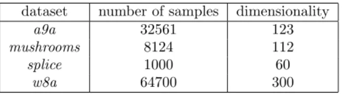
2.1 A summary of informational-hierarchic alternating direction of multiplier methods. . . 17 2.2 Summary of datasets . . . 47

(11)

List of Figures

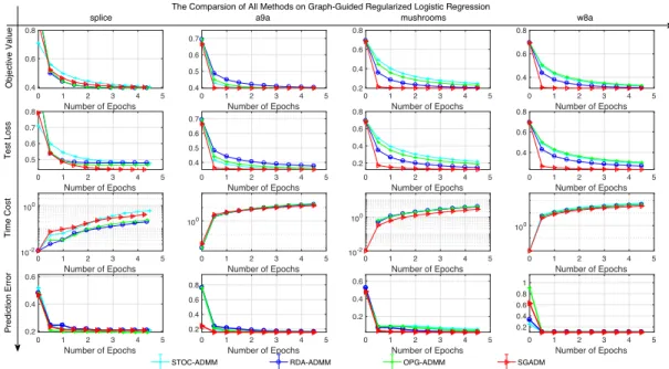
2.1 Comparison of SGADM, STOC-ADMM, RDA-ADMM, OPG-ADMM on Fused Logistic Regression. . . 48 2.2 Comparison of SGADM, STOC-ADMM, RDA-ADMM, OPG-ADMM on

Graph-guided Regularized Logistic Regression. . . 50

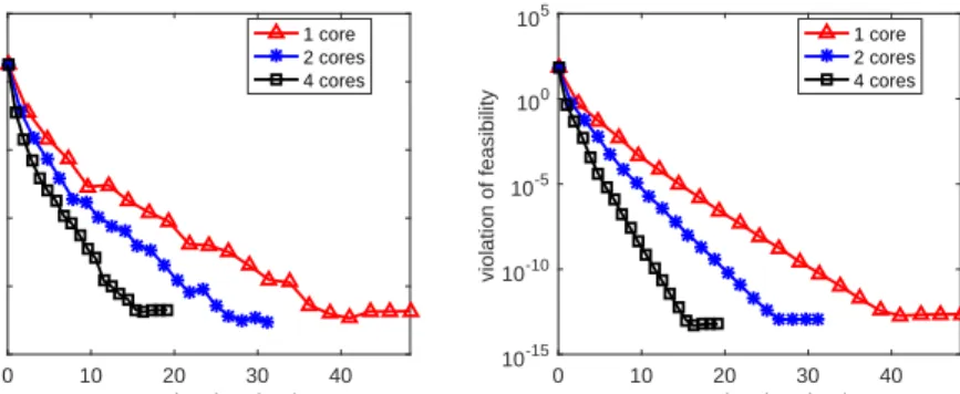
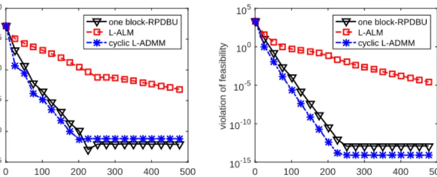
4.1 Nearly linear speed-up performance of the proposed primal-dual method for solving the nonnegativity constrained quadratic programming on a 4-core machine. . . 109 4.2 Comparison of the proposed method (RPDBU) to the linearized

aug-mented Lagrangian method (L-ALM) and the cyclic linearized alternating direction method of multipliers (L-ADMM) on solving the nonnegativity constrained quadratic programming. . . 110

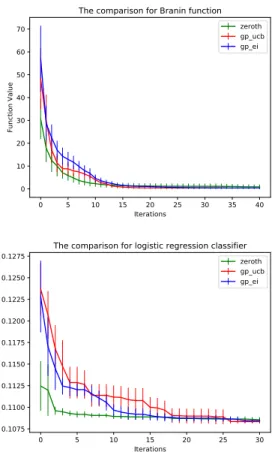
5.1 Plot of a WPC function that is not quasi-convex. . . 145 5.2 Comparisons of the zeroth-order algorithms to Bayesian optimization on

(12)

Chapter 1

Introduction

1.1 Background and Literature Review

Algorithm design is commonly considered as a central theme in the theory and practice of optimization. For continuous optimization, roughly speaking, algorithms can be classified into three types: (1) the high-order algorithms (which use the information of the Hessian or higher order derivatives of the objective function); (2) the first-order algorithms (which use no more than the gradient information of the objective function); (3) the zeroth-order algorithms (which only use the function value information). In this dissertation, we aim to present a study on the latter two types of algorithms for some specific optimization models. To distinguish from the high-order ones, let us loosely use the term low-order algorithms to represent the last two types of methods. High-order methods such as the interior point algorithms have proved to be extremely successful in solving optimization problems in general, as they typically only take a few steps to converge (cf. [6, 5]). However, there are applications arising from big data analytics that prevent high-order methods from being practical, as the computational complexity of performing one iteration of a high-order method may already be overly expensive. In those situations, the first-order methods become attractive since at each step their computational costs are substantially lower. Furthermore, in some applications only the function values are available for estimation. In such cases, the zeroth-order methods are the only choices to be considered.

As two subclasses of the lower-order algorithms, the first-order methods and the zeroth-order methods are closely related. In fact, as we will show in this dissertation, many zeroth-order methods can be derived from their well-designed first-order

(13)

coun-terpart. In the literature, two types of first-order methods are popular. The first type includes essentially the gradient algorithms and their variations, while the second type is based on the proximal gradient mappings. Consider

min

x∈_Rnf(x) (1.1)

where f(x) is a smooth convex function. The gradient method is in the form of

xk+1 =xk−αk∇f(xk), (1.2)

whereαk is the step size. Moreover, for some problems, the objective function might be

nonsmooth and there might be constraints and so the gradient method is not directly applicable. For example, consider

min

x∈Xf(x) =f0(x) +f1(x), (1.3)

whereX is a convex set, andfi is convex,i= 0,1, andf0 may be nonsmooth. This is a

typical situation where proximal type method may be relevant. In particular, we define the proximal operator prox_λf as

prox_λf(x) = arg min

y∈Xf(y) +

1

2λky−xk

2_.

For problem (1.3), the proximal point method can be described as the following iterative process

xk+1 =prox_λkf₀(xk), (1.4)

and the proximal gradient method can be described as

xk+1 =prox_λkf₀(xk−λk∇f1(xk)). (1.5)

There have been many variations originated from the proximal point and the proximal gradient methods, adapted for specific applications in various fields including engineer-ing, statistics, and economics (cf. [11]). Besides, the aforementioned gradient-type methods can also serve as a starting point for many zeroth-order methods. When the gradient information is not readily available or impractical to obtain, based on some approximations of the gradient, the corresponding zeroth-order method can still be

(14)

applied.

Given the nature of the lower-order algorithm, it is particularly useful for problems that require higher computational efficiency. In general, we study its applications for the following areas: (1) large-scale block optimization; (2) stochastic and black-box optimization; (3) online learning and online optimization. In the previous gradient-type optimization methods, the vector x is treated as a single block of variables. But in large-scale optimization problems, the dimension nis large and it would be preferable to work with some smaller-sized subproblems at each step. In fact, there are plenty of problems including matrix/tensor factorization [65, 69], group LASSO [117, 128], SVM [22] etc., where x can be decomposed as x = (x1, x2, . . . , xm)>. With such kind of

problems in mind, let us consider the following block-structured optimization model

min xi∈Xi,i=1,...,mf(x1, x2, . . . , xm) + m X i=1 ui(xi), (1.6)

wheref(·) is smooth, andui(·) may be nonsmooth. To solve this problem, it is intuitive

to utilize the block structure so that at each step of the algorithm, we only need to deal with a smaller-sized problem. To this end, the Block Coordinate Descent (BCD) method is proposed for solving problem (1.6). Basically, the BCD method tries to minimize a single block variable xi while all other blocks xj, j 6= i are fixed at each

step by following a certain selection rule of the block (e.g. cyclic, randomized, etc.). By incorporating the proximal point or proximal gradient method and implementing different block updating rule, many variants of the BCD methods have been proposed. However, for some applications, for instance the robust PCA [14], (1.6) is still not general enough. Taking the constraints into account, let us consider the following model

min xi∈Xi,i=1,...,m f(x1, x2, . . . , xm) + m P i=1 ui(xi) s.t. A1x1+A2x2+· · ·+Amxm =b, (1.7)

where Ai, i= 1, . . . , mare given matrices. For instance, by introducing a new variable,

the well-known LASSO model [117] can be transformed into (1.7):

min x∈Rn kAx−bk2₊_λ_k_x_k 1 ⇒ min x,y∈Rn kAx−bk2₊_λ_k_y_k 1 s.t. x−y= 0. (1.8)

(15)

There are in fact many applications which can be formulated in the form of (1.7) including the consensus and sharing problems, basis pursuit, compressive sensing etc.; see [7, 81, 20, 29]. For this model, the ADMM-type methods based on augmented Lagrangian have received much attention recently, which will be discussed at length later in this thesis. Unlike the deterministic large-scale optimization, for many stochastic and black-box optimizations, the lower-order algorithm seems to be the only feasible solution. A stochastic optimization problem often assumes the following structure

min

x∈Xf(x) :=E[F(x, ξ)], (1.9)

where the expectation is taken over a random variableξ. For many stochastic problems, the function F and the distribution of ξ are either very complex or unknown, which makes the higher-order information become unavailable. The black-box optimization further generalizes it into a nonparametric model where no functional form is assumed for the objective function. A good example is the hyperparameter tuning of machine learning algorithms, where the generalization error is used as the objective function. Clearly, for a given set of hyperparameters, the only possible information is the cross-validation or test error which is a noisy approximation of true generalization error. In light of this, both stochastic and black-box optimization can be viewed as the oracle-based optimization problem. For any query point x, depending on the informational structure of a problem, the corresponding feedback is given by an oracle. Moreover, the lower-order algorithm is even more powerful for solving a combination of the large-scale and the oracle-based optimization. As an extension of optimization to a changing environment, the online learning or online optimization also possesses a lower-order nature. In online learning, at each decision period t ∈ {1,2, . . . , T}, an online player chooses a feasible strategy xt from a decision set X ⊂Rn, and suffers a loss given by

ft(xt), where ft(·) is a loss function. The key feature of this framework is that the

player must make a decision for periodtwithout knowing the loss functionft(·). In this

challenging setting with limited information, the lower-order algorithms become more appropriate.

Convergence or computational complexity analysis is an indispensable part of opti-mization theory. In general, the iteration complexity is a measure of how well the algo-rithm performs after a certain number of iterations. The way to measure the quality of the current iterate varies from problem to problem, but it mainly includes the distance between the iterate and the optimal solution set, the difference between the current

(16)

function value and the optimal function value, and the violation of the optimality con-ditions. For example, if an algorithm has the iteration complexity of the orderO(1/N) in terms of the objective function value, then this means that after k iterations, the current iteratexk would satisfyf(xk)−f∗< C_k whereCis a constant. For the two fun-damental methods: the gradient method (1.2) and the proximal gradient method (1.5), the iteration complexities are well studied. In particular, the gradient method has been shown an iteration complexity of O(1/N) (cf. [6]). Moreover, [86] shows that the com-plexity can be further improved toO(1/N2) by an acceleration procedure and this is the optimal rate that any gradient-type method can possibly achieve, and if the function is strongly convex then the method actually converges linearly. For the proximal gradient method, similar results hold: the O(1/N) complexity of the original method, which can be accelerated to an O(1/N2) iteration complexity; see [3, 87, 88, 120]. For prob-lem (1.6), extensive research of the iteration complexity of the BCD-type method has been reported in the literature. Under different conditions, the sublinear convergence

rate O(1/N) or the linear rate can be achieved for the block minimization BCD-type

methods (cf. [79, 125, 60]). Furthermore, for the proximal gradient BCD-type method, [90, 100, 77, 4, 60] show that the similar convergence rate can still be established.

In this Ph.D. thesis, we study the first-order and zeroth-order methods for op-timization models around the following themes: the iteration complexity analysis of different ADMM-type algorithms for solving various block optimization problems, and the analysis of lower-order gradient-type algorithms for solving oracle-based black-box optimization and online optimization.

Instead of aiming to solve the general multi-block model (1.7), the basicAlternating Direction Method of Multipliers (abbreviated as ADMM) is originally designed to solve the following two-block constrained convex optimization model

min f(x) +g(y)

s.t. Ax+By =b,

x∈ X, y∈ Y

(1.10)

where x∈_Rnx_,_y _∈

Rny, A∈Rm×nx,B ∈Rm×ny,b∈Rm, and X ⊆Rnx,Y ⊆Rny are

closed convex sets; f and g are convex functions.

An intensive recent research attention for solving problem (1.10) has been devoted to the ADMM, which is known to be a manifestation of the operator splitting method (cf. [30, 33, 46] and the references therein). Large-scale optimization problems in the

(17)

form of (1.10) can be found in many application domains including compressed sensing, imaging processing, and statistical learning. Due to the large-scale nature, it is often impossible to inquire the second order information (such as the Hessian of the objective function) or invoke any second order operations (such as inverting a full-scale matrix) in the solution process. In this context, the ADMM as a first order method is an attractive approach; see [10]. Specifically, for solving (1.10), a typical iteration of ADMM proposed in [46] runs as follows:      xk+1 = arg minx∈XLγ(x, yk, λk) yk+1 _{= arg min} y∈YLγ(xk+1, y, λk) λk+1 =λk−γ(Axk+1+Byk+1−b), (1.11)

where L_γ(x, y, λ) is the augmented Lagrangian function for problem (1.10) defined as:

Lγ(x, y, λ) =f(x) +g(y)−λ>(Ax+By−b) +

γ

2kAx+By−bk

2_. _(1.12)

The convergence of the ADMM for (1.10) is actually a consequence of the convergence of the so-called Douglas-Rachford operator splitting method (see [45, 33]). However, the rate of convergence for ADMM is established only very recently: [57] shows that for problem (1.10) the ADMM converges at the rate ofO(1/N) whereN is the number of total iterations. From the perspective of monotone inclusion, a similar iteration complexity is also obtained in [80] under different assumptions. Moreover, a non-ergodic

O(1/N) iteration complexity in terms of the infeasibility measure and the objective value

are found very recently in [56, 74, 26]. Furthermore, by imposing additional conditions on the objective function or constraints, the ADMM can be shown to converge linearly; see [48, 28, 59, 8, 73]. Moreover, as we will show later in this thesis, the ADMM framework can be naturally extended to solve problems with more than two blocks of variables.

Besides the multi-block structure, we can take a different stance towards the applica-bility of the ADMM, depending on the prevailing information structure of the problem. Observe that to implement (1.11), it is necessary that arg minx∈XLγ(x, yk, λk) and

arg miny∈YLγ(xk+1, y, λk) can be solved efficiently at each iteration; i.e. the proximal

mappings are assumed to be easy. While this is indeed the case for some classes of the problems (e.g. the lasso problem), it may also fail for many other applications. This triggers a natural question: Given the structure of the objective functions in the

(18)

mini-mization subroutines, can the multipliers’ method be adapted accordingly? In Chapter 2, we study some variants of the ADMM based on incorporating the two basic first-order methods (1.2) and (1.5) to account for this informational structure of the objective func-tions. One possible scenario is that it is not easy to solve the subproblems of x and y in (1.11), in this case, we can introduce the gradient projection method (a special form of proximal gradient method) to replace the exact minimization subproblem. In particular, this leads to two algorithms: one is the GADM (Gradient-ADM, replacing the subproblem of one block by gradient method) and the other is GALM (Gradient-ALM, replacing the subproblems of both blocks by gradient method), and those two algorithms will further allow us to deal with different informational structure of the problem.

To take into account the informational structure, one natural way is to consider the stochastic setting of problem (1.10), where we can go beyond the deterministic in-formational structure of the problem. In stochastic programming (SP), the objective function is often in the form of expectation. In this case, even requesting its full gra-dient information is impractical. Historically, Robbins and Monro [102] introduced the so-called stochastic approximation (SA) approach to tackle this problem. Polyak and Juditsky [96, 97] proposed an SA method in which larger step-sizes are adopted and the asymptotical optimal rate of convergence is achieved; cf. [34, 37, 105, 104] for more details. Recently, there has been a renewed interest in SA, in the context of compu-tational complexity analysis for convex optimization [85], which has focussed primarily on bounding the number of iterations required by the SA-type algorithms to ensure the expectation of the objective to be away from optimality. For instance, Nemirovski et al. [83] proposed a mirror descent SA method for the general nonsmooth convex stochastic programming problem attaining the optimal convergence rate of O(1/√N); Lan and his coauthors [43, 41, 40, 42, 68, 44] proposed various first-order methods for SP problems under suitable convex or non-convex settings. In [93], a stochastic version of problem (1.10) is considered. In this proposal we also consider the GADM and the GALM in the SP framework. Under the stochastic framework, the informational struc-ture of the problem appears in a progressive way. To start with, we first assume that a noisy gradient information of the function is available. Thus, in our GADM method or GALM method, we can only use a noisy stochastic estimate of the gradient and we name those methods as SGADM (stochastic-ADM) and SGALM (stochastic-ALM). Furthermore, it is possible that even the noisy gradient information is not available. In

(19)

this case, we assume that we can only get the noisy estimation of the function value, and this gives us an avenue where the zeroth-order method can apply. Inspired by the work of Nesterov [89] for gradient-free minimization, we will propose a zeroth-order (gradient-free, a.k.a. direct) smoothing method for (1.10). Specifically, we show that the SGADM and the SGALM can be extended to the zeroth-order version by incorporating the zeroth-order gradient estimate into the algorithms.

So far we have discussed the different variants of ADMM for solving problem (1.10) which is a special case of the problem (1.7). Is it possible to extend the ADMM frame-work to the more general problem (1.7) where we have both multi-block variables and coupled the objective function f(x1, x2, . . . , xm)? The answer is positive, and we will

discuss this thoroughly in Chapter 3 and Chapter 4. In fact, utilizing the multi-block structure of the problem, the multi-block ADMM updates the block variables sequen-tially. Specifically, it performs the following updates iteratively (by assuming the ab-sence of the coupled functions f):

           xk₁+1 = arg minx1∈X1Lρ(x1, x k 2,· · ·, xkm, λk), .. . xk_m+1 = arg minxm∈XmLρ(xk1+1,· · · , x k+1 m−1, xm, λk), λk+1 = λk−γ(A1xk1+1+A2xk2+1+· · ·+Amxkm+1−b), (1.13)

where the augmented Lagrangian function is similarly defined as:

L_γ(x, λ) = m X i=1 ui(xi)−λ> m X i=1 Aixi−b ! +γ 2 m X i=1 Aixi−b 2 . (1.14)

Although the multi-block ADMM scheme in (1.13) performs very well for many instances encountered in practice (e.g. [94, 116]), it may fail to converge for some instances if there are more than 2 blocks of variables, i.e., m ≥ 3. In particular, an example was presented in [16] to show that the ADMM may even diverge with 3 blocks of variables, when solving a linear system of equations. Thus, some additional assumptions or modifications will have to be in place to ensure convergence of the multi-block ADMM. In fact, by incorporating some extra correction steps or changing the Gauss-Seidel updating rule, [27, 55, 54, 52, 124] show that the convergence can still be achieved for the multi-block ADMM. Moreover, if some part of the objective function is strongly convex or the objective has certain regularity property, then it can be shown

(20)

that the convergence holds under various conditions; see [17, 74, 13, 73, 70, 47, 123]. Using some other conditions including the error bound condition and taking small dual stepsizes, or by adding some perturbations to the original problem, authors of [59, 75] establish the rate of convergence results even without strong convexity. Not only for the problem with linear constraint, in [19, 71, 112] multi-block ADMM are extended to solve convex linear/quadratic conic programming problems. In a recent work [113], the authors propose a randomly permuted ADMM (RP-ADMM) that basically chooses a random permutation of the block indices and performs the ADMM update according to the order of indices in that permutation, and they show that the RP-ADMM converges in expectation for solving non-singular square linear system of equations.

In [58], the authors propose a block successive upper bound minimization method of multipliers (BSUMM) to solve problem (1.7). Essentially, at every iteration, the BSUMM replaces the nonseparable part f(x) by an upper-bound function and works on that modified function in an ADMM manner. Under some error bound conditions and a diminishing dual stepsize assumption, the authors are able to show that the iterates produced by the BSUMM algorithm converge to the set of primal-dual optimal solutions. Along a similar direction, Cui et al. [23] introduces a quadratic upper-bound function for the nonseparable functionf to solve 2-block problems; they show that their algorithm has an O(1/N) convergence rate, where t is the number of total iterations. Moreover, [18] shows the convergence of the ADMM for 2-block problems by imposing quadratic structure on the coupled functionf(x) and also the convergence of RP-ADMM for multi-block case where all separable functions vanish (i.e. ui(xi) = 0,∀i).

In Chapter 3, we study the ADMM and its variants for (1.7). (Some adaptations of the ADMM are particularly relevant if there is a coupling term in the objective, as the minimization subroutines required by the ADMM may become difficult to implement; see more discussions on this later.) Instead of using some upper-bound approximation (a.k.a. majorization-minimization), we work with the original objective function. In some applications, it is difficult or impossible to implement the ADMM iteration, be-cause the augmented Lagrangian function in (1.11) may be difficult to optimize even if the other block of variables and the Lagrangian multipliers are fixed. This motivates us to propose theAlternating Proximal Gradient Method of Multipliers (APGMM), which essentially iterates between proximal gradient methods of each block variables before the multiplier is updated. If optimizing the augmented Lagrangian function for one block of variables is easy while optimizing the other block of variables is difficult, then a hybrid

(21)

between ADMM and APGMM is a natural choice. What if the gradient proximal sub-routines are still too difficult to be implemented? One would then opt to compute the gradient projections. Hence, we propose the Alternating Gradient Projection Method of Multipliers (AGPMM), which replaces the proximal gradient steps in APGMM by the gradient projections. At this stage, all the methods mentioned above are considered in the context of the 2-block model. In general however, they can be extended to the multi-block model with a coupling term.

In Chapter 4, we study a more general model that includes (1.7) as a special case. Specifically, we introduce another set of variablesy which has a similar mixed structure (coupled and separate) as x in (1.7). We propose a randomized primal-dual coordinate update algorithm by introducing randomization to the multi-block ADMM framework (1.13). Different from the random permutation scheme in [113, 18], a simpler variable selection rule based on uniform distribution is used. The randomization is crucial to the convergence of the algorithm. In fact, the randomization scheme enables us to establish the O(1/N) convergence rate for this coupled multi-block model with mere convexity. The way we deal with the coupled objective function is to use proximal gradient approach, and it has two additional benefits. First, by incorporating a properly chosen proximal term, the variables can be decoupled and the algorithm can be done in parallel. Furthermore, the proximal gradient (linearization) scheme can be adapted to solve stochastic optimization problems. In fact, based on the informational structure of the coupled function f, an approximation of the gradient can be obtained. The randomized primal-dual coordinate update can still be readily implemented, given an unbiased approximation is available under some oracle-based models.

Besides the multi-block optimization problem, low-order algorithms are also suit-able for solving black-box optimization and bandit online learning problem. For both of the problems, the key feature is that no higher-order information is available other than the function value estimation. In optimization, solution procedures using only objective values are often referred to as direct methods. In [99], Powell (1964) con-structed a method based on conjugate directions for quadratic minimization; in [82], Nelder and Mead (1965) introduced the so-called simplex method for nonlinear opti-mization, while justifications for the simplex method in low dimensions can be found in [67, 66]. A modern account and historical notes of the direct methods can be found in a recent book ([21]) by Conn, Scheinberg, and Vicente. Our study however, builds on a relatively recent approach of randomized zeroth-order approximation of the

(22)

gra-dient, pioneered by Nesterov and Spokoiny [89]; some of the ideas in the approach can be traced back to Polyak [98]. As a different type of optimization method, Bayesian optimization [63] also provides a powerful tool for black-box optimization. In general, Bayesian optimization constructs a prior probabilistic distribution over the functional space. When the data are observed, it sequentially refines this model using Bayesian posterior distribution. The procedure finds the next query point by maximizing an ac-quisition function induced by the corresponding probabilistic model. For more details and applications about Bayesian Optimization, see, e.g., [12, 108, 111]. From a different perspective, there has been a great research interest in using the lower-order method for online learning problem. Several sub-linear cumulative regret bounds measured by stationary regret have been established in various papers in the literature. For example, [131] proposed an online gradient descent algorithm which achieves an regret bound of order O(√T) for convex loss functions. The order of the regret can be further improved

to O(logT) if the loss functions are strongly convex (see [49]). Moreover, the bounds

are shown to be tight for convex / strongly convex loss functions respectively in [1]. In the so-called bandit online convex optimization, where the online player is only sup-posed to know the function valueft(xt) atxt, instead of the entire functionft(·). When

the player can only observe the function value at a single point, [35] established an O(T3/4) regret bound for general convex loss functions by constructing a zeroth-order approximation of the gradient. Assuming that the loss functions are smooth, the regret bound can be improved to O(T2/3) by incorporating a self-concordant regularizer (see [106]). Alternatively, if multiple points can be inquired at the same time, [2] showed that the regrets can be further improved to O(T1/2_{) and}_O(log_{T) for convex / strongly}

convex loss functions respectively. In this dissertation, we study various zeroth-order algorithms for the black-box optimization and online learning. In particular, we study the optimization models under three different settings. In the first setting, the model is basically stochastic programming with the following side restriction: similar to the online bandit learning framework, only one random sample can be drawn at any given decision point. In the second setting, we present a general nonconvex optimization framework (weakly pseudo convex), and develop a specialized zeroth-order normalized gradient method. In the third setting, the objective value can be estimated arbitrarily close to the true value, at a cost that is increasing with regard to the inverse of the pre-cision desired. Furthermore, we extend the analysis to a general constrained model with a composite objective function, consisting of the original objective and a non-smooth

(23)

regularizer. The above-mentioned settings are considered respectively for that general case as well, extending the sample complexity analysis under a proximal gradient dom-inance assumption. In Chapter 6, we further extend the similar idea to the stochastic bandit online learning problem, where the nonsmoothness of the loss function and the one random sample scheme are discussed.

1.2 Overview and Organization

In Chapter 2, we present a suite of variants of the ADMM, including GADM, GALM, SGADM, SGALM, and the zeroth-order version of SGADM and SGALM. Clearly, the new variants allow the method to be applicable on a much broader class of problems where only noisy estimations of the gradient or the function values are accessible, yet the flexibility is achieved without sacrificing the computational complexity bounds. In fact, we will show that the rate of convergence of GADM and SGADM would be O(1/N) and O(1/√N) respectively, and show SGALM admits a similar iteration complexity bound. Moreover, we will show that the zeroth-order SGADM and SGALM also have the O(1/√N) complexity.

In Chapter 3, we first study the 2-block case of the optimization model (1.7), where we analyze the proposed first-order algorithms to solve this model. First, the ADMM is extended, assuming that it is easy to optimize the augmented Lagrangian function with one block of variables at each time while fixing the other block. We prove thatO(1/N) iteration complexity bound holds under suitable conditions. If the subroutines of the ADMM cannot be implemented, then our APGMM, AGPMM, and the hybrids of them may be still applicable. Under suitable conditions, the O(1/N) iteration complexity bound is shown to hold for all the newly proposed algorithms. Finally, we extend the analysis for the ADMM to the general multi-block case.

In Chapter 4, we propose a randomized primal-dual proximal block coordinate up-dating framework for a general multi-block convex optimization model with coupled objective function and linear constraints. Assuming mere convexity, we establish its

O(1/N) convergence rate in terms of the objective value and feasibility measure. Our

analysis recovers and/or strengthens the convergence properties of several existing algo-rithms. In particular, Our result shows that a sublinear rate of convergence in expecta-tion can be guaranteed for multi-block ADMM, without assuming any strong convexity. The new approach is also extended to solve problems where only a stochastic

(24)

approxi-mation of the (sub-)gradient of the objective is available, and we establish anO(1/√N) convergence rate of the extended approach for solving stochastic programming.

In Chapter 5, we first study an unconstrained stochastic optimization model where the objective can be allowed a single-sample at a point. The convergence analysis also extends to the star-convex functions. Moreover, we consider a class of nonconvex optimization model by introducing the so-called weak pseudo-convexity. For this model, we develop a zeroth-order normalized gradient descent method. For the aforementioned two models, we show the sublinear convergence rate of our zeroth-order methods. In addition, we study unconstrained optimization where only the objective function can be estimated, and the efforts required to estimate the function value depends on the precision. Finally, we extend our investigations to the constrained optimization with a regularization function. Linear convergence rate is derived for the latter two models under strong convexity and gradient dominance respectively.

In Chapter 6, we present the zeroth-order methods for solving online learning prob-lem. Specifically, we study the online convex optimization with stochastic loss functions. The goal is to design some effective algorithms such that the total regret will be bounded above nontrivially by the time horizon T. In fact, we propose a stochastic gradient de-scent method under this setting. We prove the O(√T) regret bound for both smooth and non-smooth loss functions and the O(T34) regret bound for non-smooth stochastic

(25)

Chapter 2

Information-Adaptive Variants of

the ADMM

2.1 Introduction

In this chapter, we consider the most basic ADMM model:

min f(x) +g(y) s.t. Ax+By =b, x∈ X, y∈ Y (2.1) where x ∈ _Rnx_, _y _∈ Rny, A ∈ Rm×nx, B ∈ Rm×ny, b ∈ Rm, and X ⊆ Rnx,Y ⊆ Rny

are closed convex sets; f is a smooth convex function, andg is a convex function and possibly nonsmooth. We further assume that the gradient of f is Lipschitz continuous:

k∇f(x)− ∇f(y)k ≤Lkx−yk, ∀x, y∈ X, (2.2)

where Lis a Lipschitz constant.

Recall, the augmented Lagrangian function for problem is defined as:

Lγ(x, y, λ) =f(x) +g(y)−λ>(Ax+By−b) +

γ

2kAx+By−bk

2_. _(2.3)

To bring out the hierarchy regarding the available information of the functions in question, let us first introduce the following definition.

(26)

Definition 1 We call a convex function f(x) to be easy to minimize with respect to x

(f is hence said to be MinE as an abbreviation) if there exits some H 0 such that the proximal mapping arg minxf(x) + 1₂kx−zk2H can be computed easily for any given

z.

Some remarks are in order here. If L_γ(x, y, λ) is MinE with respect to both x and y with H= 0, then the original ADMM (1.11) is readily applicable. For the cases where

Lγ(x, y, λ) isMinEwith respect to bothx and ybutH is nonzero, the convergence of

different inexact ADMM-type methods have been studied in [51, 92, 53]. Moreover, [110, 15, 59] show that by incorporating various modifications of ADMM with the proximal method an O(1/N) convergence rate can still be achieved. In the case thatL_γ(x, y, λ) isMinEinxbut not iny, Lin, Ma and Zhang [72] recently proposed an extra-gradient ADMM (EGADM) and showed anO(1/N) iteration bound. In this chapter, we consider a simpler procedure of applying gradient only once in each iteration (to be named GADM):     

yk+1 = arg miny∈YLγ(xk, y, λk) +1₂ky−ykk2_H

xk+1= [xk− ∇xLγ(xk, yk+1, λk)]X

λk+1 =λk−γ(Axk+1+Byk+1−b),

(2.4)

where [x]X denotes the projection ofxontoX. In fact, a variant of above procedure was

considered in [72], where x is updated by taking the gradient of Lagrangian function rather than augmented Lagrangian function, and it was posed as an unsolved problem to determine the iteration complexity bound of this modified algorithm. In this chapter we prove that the GADM also has an iteration bound of O(1/N). Moreover, our analysis does not require the optimal set to be bounded nor the coercivity of the objective function, which is key to obtaining iteration bounds in many previous works; see [32, 28, 72, 84]. In addition to the assumptions made at the beginning of this section, throughout the chapter we only assume:

Assumption 2.1.1 The optimal solution set X∗× Y∗ for problem (2.1) is non-empty.

Under this assumption, naturally we have dist(x,X∗)M := minu∈X∗kx−uk_M <∞, and

dist(y,Y∗₎

M := minv∈Y∗ky−vk_M <∞, for any given x, yand matrixM 0.

In this chapter we also consider (2.4) in the SP framework. We assume that a noisy gradient information of ∇Lγ via the so-called stochastic first order oracle (SF O) is

(27)

a stochastic gradient G(x, ξ) from the SF O, where ξ is a random variable following a certain distribution. Formally we introduce:

Definition 2 We call a function f(x) to be easy for gradient estimation – denoted as GraE– if there is anSF Oforf, which returns a stochastic gradient estimationG(x, ξ)

for ∇f atx, satisfying

E[G(x, ξ)] =∇f(x), (2.5)

and

E[kG(x, ξ)− ∇f(x)k2]≤σ2. (2.6)

If the exact gradient information is available then theSF Ois deterministic. In gen-eral, the SF O is often stochastic and inaccurate. For instance, the stochastic gradient that is used in many machine learning algorithms can be viewed as a special case of

SF Owhere the distribution is uniform on the dataset. As for problem (2.1), quite a few ADMM variants in stochastic and online optimization setting have been proposed re-cently; see [93, 121, 114, 115, 129, 130]. The basic idea in those works is to linearize the stochastic function and use the noisy gradient in the subproblem. In [93, 121, 114, 129], theO(1/√N) andO(lnN/N) iteration complexities have been shown for general convex function and strongly convex function respectively. Moreover, [130] shows an O(1/N) iteration complexity can be achieved if an incremental approximation of the full gradient is used. By assuming both functions are strongly convex and smooth, a linear conver-gence is shown in [115]. In this chapter, whenL_γ(x, y, λ) isMinEwith respect toy, and f(x) in (2.3) is GraE, we will then propose a stochastic gradient ADMM (SGADM), which alternates through one exact minimization step ADMM (1.11), one stochastic approximation iteration, and an update on the dual variables (multipliers). It is clear that the SGADM in the deterministic case is exactly GADM (2.4), and we will show that the rate of convergence of GADM and SGADM would be O(1/N) and O(1/√N) respectively. n particular, if f(x) is strongly convex, the complexity of SGADM can be improved to O(lnN/N). Moreover, if f(x) and g(y) in (2.3) are both GraE, then we propose a stochastic gradient augmented Lagrangian method (SGALM), and show that it admits a similar iteration complexity bound.

Furthermore, we are also interested in another class of stochastic problems, where even the noisy gradient information is not available; instead we assume that we can only get a noisy estimation of f via the so-calledstochastic zeroth-order oracle (SZO). Specifically, for any input x, by calling SZO once it returns a quantity F(x, ξ), which

(28)

is a noisy approximation of the true function value f(x). More specifically,

Definition 3 We call a function f(x) to be easy for function evaluation – denoted as ValE – if there is an SZO for f, which returns a stochastic estimation for f at x if

SZO is called, satisfying

E[F(x, ξ)] =f(x), (2.7)

E[∇F(x, ξ)] =∇f(x), (2.8)

and

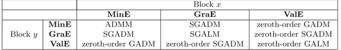
E[k∇F(x, ξ)− ∇f(x)k2]≤σ2. (2.9) Inspired by the work of Nesterov [89] for gradient-free minimization, in this chapter we will propose a zeroth-order (gradient-free, a.k.a. direct) smoothing method for (2.1). Instead of using the Gaussian smoothing scheme as in [89], which has an unbounded support set, we apply another smoothing scheme based on theSZOoff. To be specific, whenL_γ(x, y, λ) isMinEwith respect toy, andf(x) in (2.3) isValE, we will propose a zeroth-order gradient augmented Lagrangian method (zeroth-order GADM) and analyze its complexity. To summarize, according to the available informational structure of the objective functions, in this chapter we present suitable variants of the ADMM to account for the available information. In a nutshell, the details are in the following Table 2.1.

Blockx

MinE GraE ValE

Blocky

MinE ADMM SGADM zeroth-order GADM

GraE SGADM SGALM zeroth-order SGADM

ValE zeroth-order GADM zeroth-order SGADM zeroth-order GALM

Table 2.1: A summary of informational-hierarchic alternating direction of multiplier methods.

The rest of the chapter is organized as follows. In Section 2.2, we propose the stochastic gradient ADMM (SGADM) algorithm, and analyze its complexity. In Sec-tion 2.3, we present our stochastic gradient augmented Lagrangian method (SGALM) which uses gradient projection in both block variables, and analyze its convergence rate. In Section 2.4, we propose a zeroth-order GADM through a new smoothing scheme, and present a complexity result. Finally, we present some numerical experiment results in Section 2.5.

(29)

2.2 The Stochastic Gradient Alternating Direction of

Mul-tipliers

In this section, we assume Lγ(x, y, λ) to be MinE with respect to y, and f(x) to be GraE. That is, for a givenx, whenever we need∇f(x), we can actually get a stochastic gradientG(x, ξ) from theSF O, whereξ is a random variable following a certain distri-bution. Moreover, G(x, ξ) satisfies (2.5) and (2.6). By the definition of the augmented Lagrangian Lγ(x, y, λ), anSF OforLγ(x, y, λ) can be constructed accordingly:

Definition 4 Denote theSF O of ∇xLγ(x, y, λ) as GL(x, y, λ, ξ), which is defined as:

GL(x, y, λ, ξ) :=G(x, ξ)−A>λ+γA>(Ax+By−b). (2.10)

One example where such application arises isstochastic lasso problem: min x 1 2Eξ(a > ξx−bξ)2+µkxk1,

where the sensing vectoraξas well as the sensing resultbξ are given stochastically. The

problem can be formulated as

min 1₂Eξ(a>ξx−bξ)2+µkyk1

s.t. x−y= 0.

Assuming each time one sample is observed, we have G(x, ξ) =aξ(a>ξx−bξ).

Our first algorithm to be introduced, SGADM, works as follows:

The Stochastic Gradient ADMM (SGADM) Initializex0∈ X, y0∈ Y andλ0 fork= 0,1,· · ·,do yk+1 _{= arg min} y∈YLγ(xk, y, λk) +₂1ky−ykk2H; xk+1= [xk−αkGL(xk, yk+1, λk, ξk+1)]X; λk+1=λk−γ(Axk+1+Byk+1−b). end for

In the above notation, [x]X denotes the projection ofxonto X,H is a pre-specified

positive semidefinite matrix, αk is the stepsize for the k-th iteration. In fact, matrix

(30)

in order for the resulting subproblem to be separable, or even to admit a closed-form solution. In our proposed algorithms, the H matrix can be set to 0 which recovers the original ADMM subproblem. It is easy to see that the deterministic version of SGADM is exactly GADM (2.4). The above SGADM is similar to the stochastic ADMM proposed in [93], where anO(1/√N) iteration complexity is shown. The difference lies in the fact that the SGADM linearizes the whole augmented Lagrangian and performs a gradient projection, while [93] linearizes the objective function in the augmented Lagrangian and minimizes the resulting function. We note that the OPG-ADMM in [114] also linearizes the whole augmented Lagrangian, but the order of updating blocks is different. In OPG-ADMM, it first updates the block with a gradient-type step and then updates the other block by exact minimization, while in our algorithm the order is reversed. In the following subsection, based on the measure of the constraint violation and the gap of objective value, we will show that the complexity of SGADM is O(1/√N) and the complexity of GADM is O(1/N). Furthermore, if the function f is strongly convex, it can be shown that the complexity of SGADM is indeed O(lnN/N).

2.2.1 Convergence Rate Analysis of the SGADM

In this subsection, we shall analyze the convergence rate of SGADM algorithm. First, some notations and preliminaries are introduced to facilitate the discussion.

Preliminaries and Notations

Denote u= y x ! , w=    y x λ   , F(w) =    −B>λ −A>λ Ax+By−b   , (2.11)

h(u) =f(x) +g(y), Ω =Y × X ×_Rm_{, and}

Qk=    H 0 0 0 _α1 kInx 0 0 −A 1 γIm   , P=    Iny 0 0 0 Inx 0 0 −γA Im   , Mk=    H 0 0 0 _α1 kInx 0 0 0 1 γIm   . (2.12)

(31)

Clearly, Qk =MkP. In addition to the sequence {wk} generated by the SGADM, we

introduce an auxiliary sequence:

˜ wk:=    ˜ yk ˜ xk ˜ λk   =    yk+1 xk+1 λk−γ(Axk+Byk+1−b)   . (2.13)

Based on (2.13) and (2.12), the relationship between the new sequence {w˜k} and the original {wk}is

wk+1 =wk−P(wk−w˜k). (2.14) The above succinct notations and analysis framework were originally introduced and used by He and Yuan in [57]. In this chapter, we adopt the same framework for analysis following that of [57]; in other words, our convergence result is also based on the auxiliary sequence ˜wk. Moreover, we denote δk ≡G(xk−1, ξk)− ∇f(xk−1), which is the error of

the noisy gradient generated bySF O. The following lemma is straightforward.

Lemma 2.2.1 For anyw0, w1,· · ·, wN−1, letF be defined in (2.11)andw¯= _N1

N−1 P k=0 wk; then it holds ( ¯w−w)>F( ¯w) = 1 N N−1 X k=0 (wk−w)>F(wk). Proof. Since F(w) =    0 0 −B 0 0 −A A B 0       y x λ   −    0 0 b  

,for any w1 andw2 we have (w1−w2)>(F(w1)−F(w2)) = 0. (2.15)

(32)

Therefore, ( ¯w−w)>F( ¯w) (2.15)₌ ( ¯w−w)>F(w) = 1 N N−1 X k=0 wk−w !> F(w) = 1 N N−1 X k=0 (wk−w)>F(w) (2.15) = 1 N N−1 X k=0 (wk−w)>F(wk). (2.16)

The Complexity of SGADM without Strong Convexity

We now present the rate of convergence result for SGADM, which is O(1/√N). Denote

Ξk = (ξ1, ξ2, . . . , ξk). In fact, the convergence rate is in the sense of the expectation

taken over Ξk.

Theorem 2.2.2 Suppose thatL_γ(x, y, λ)isMinEwith respect toy, andf(x)isGraE. Given a fixed iteration number N, lettingwk be the sequence generated by the SGADM, and choosing ηk=

√

N, and C >0 be a constant satisfying CInx −γA>A−LInx 0, and αk= _ηk1₊_C = √_N1₊_C. Let ¯ wn:= 1 n n−1 X k=0 ˜ wk, (2.17)

where w˜k is defined in (2.13). Then the following holds

EΞN[h(¯uN)−h(u ∗ ) +ρkA¯xN +By¯N −bk] ≤ 1 2√N(σ 2₊_D2 x) + 1 2N D2_y,H+CD2_x+ 1 γ ρ+kλ 0_k2 , (2.18)

where Dx = dist(x0,X∗), Dy,H = dist(y0,Y∗)H and ρ is any given positive number.

As in [57], we first present a bound regarding the sequence{w˜k} in (2.13).

(33)

given in (2.12). For any w∈Ω, we have h(u)−h(˜uk) + (w−w˜k)>F( ˜wk) ≥ (w−w˜k)>Qk(wk−w˜k)−(x−xk)>δk+1− kδk+1k2 2ηk −ηk+L 2 kx k₋_x_˜k_k2_, (2.19)

whereηk>0is any constant. Moreover, for anyw∈Ω, the term(w−w˜k)>Qk(wk−w˜k) on the RHS of (2.19) can be further bounded below as follows

(w−w˜k)>Qk(wk−w˜k) ≥ 1 2 kw−wk+1k2_Mk − kw−wkk2_Mk+1 2(x k₋_x_˜k₎> 1 αk Inx−γA>A (xk−x˜k). (2.20)

The proof of Proposition 2.2.3 involves several steps. In order not to distract the flow of presentation, we delegate its proof to the appendix.

Proof of Theorem 2.2.2

Proof. Recall that CInx −γA>A−LInx 0 and αk= _ηk1₊_C. By (2.19) and (2.20),

h(u)−h(˜uk) + (w−w˜k)>F( ˜wk) ≥ 1 2 kw−wk+1k2_Mk− kw−wkk2_Mk+1 2(x k₋_x_˜k₎> 1 αk Inx−γA>A (xk−x˜k) −(x−xk)>δk+1− kδk+1k2 2ηk −ηk+L 2 kx k₋_x_˜k_k2 = 1 2 kw−wk+1k2 Mk− kw−wkk2Mk +1 2(x k₋_x_˜k₎> 1 αk Inx−γA>A−(ηk+L)Inx (xk−x˜k) −(x−xk)>δk+1− kδk+1k2 2ηk ≥ 1 2 kw−wk+1k2_Mk− kw−wkk2_Mk−(x−xk)>δk+1− kδk+1k2 2ηk . (2.21)

(34)

Using the definition of Mk, from (2.21) we have h(˜uk)−h(u) + ( ˜wk−w)>F( ˜wk) ≤ 1 2 ky−ykk2 H − ky−yk+1k2H + 1 2γ kλ−λkk2_{− k}_λ₋_λk+1_k2 +kx−x k_k2_{− k}_x₋_xk+1_k2 2αk + (x−xk)>δk+1+ kδk+1k2 2ηk . (2.22)

Summing up the inequalities (2.22) for k= 0,1, . . . , N−1 we have

h(¯uN)−h(u) + ( ¯wN −w)>F( ¯wN) ≤ 1 N N−1 X k=0 h(˜uk)−h(u) + 1 N N−1 X k=0 ( ˜wk−w)>F( ˜wk) ≤ 1 2N N−1 X k=0 kx−xkk2_{− k}_x₋_xk+1_k2 αk + 1 N N−1 X k=0 (x−xk)>δk+1+ kδk+1k2 2ηk + 1 2N ky−y0k2 H + 1 γkλ−λ 0_k2 , (2.23)

where the first inequality is due to the convexity ofh and Lemma 2.2.1.

Note the above inequality is true for allx∈ X, y∈ Y, and λ∈_Rm_{, hence it is also}

true for any optimal solution x∗, y∗, and B_ρ = {λ: kλk ≤ρ}. As a result, by letting w∗= (x∗, y∗, λ)>, it follows that sup λ∈Bρ h h(¯uN)−h(u∗) + ( ¯wN −w∗)>F( ¯wN) i = sup λ∈Bρ h h(¯uN)−h(u∗) + (¯xN−x∗)>(−A>λ¯N) + (¯yN−y∗)>(−B>λ¯N) +(¯λN −λ)>(A¯xN+By¯N −b) i = sup λ∈Bρ h h(¯uN)−h(u∗) + ¯λ>N(Ax ∗₊_By∗₋_b)₋_λ>_(A¯_x N +By¯N−b) i = sup λ∈Bρ h h(¯uN)−h(u∗)−λ>(Ax¯N +By¯N −b) i = h(¯uN)−h(u∗) +ρkAx¯N +By¯N −bk, (2.24)

(35)

where w∗ = (x∗, y∗, λ)>. Combining (2.23) and (2.24), we have h(¯uN)−h(u∗) +ρkAx¯N +By¯N −bk ≤ 1 2N N−1 X k=0 kx∗−xkk2_{− k}_x∗₋_xk+1_k2 αk + 1 N N−1 X k=0 (x∗−xk)>δk+1+ kδk+1k2 2ηk + 1 2N ky ∗₋_y0_k2 H + 1 γ λ∈Bρsup kλ−λ0k2 ! . (2.25)

Moreover, since αk = _ηk1₊_C = √_N1₊_C, it follows that N−1 X k=0 kx∗−xkk2_{− k}_x∗₋_xk+1_k2 αk = N−1 X k=0 (√N +C)(kx∗−xkk2_{− k}_x∗₋_xk+1_k2₎ ≤ ( √ N+C)kx∗−x0k2. (2.26)

Now, by plugging (2.26) into (2.25) and choosing x∗, y∗ such thatDx =kx∗−x0k and

Dy,H =ky∗−y0kH, it yields h(¯uN)−h(u∗) +ρkA¯xN +By¯N −bk ≤ 1 N N−1 X k=0 (x∗−xk)>δk+1+ kδk+1k2 2ηk + 1 2√Nkx ∗₋_x0_k2 + 1 2N ky ∗₋_y0_k2 H +Ckx∗−x0k2+ 1 γ λ∈Bρsup kλ−λ0k2 ! ≤ 1 N N−1 X k=0 (x∗−xk)>δk+1+ kδk+1k2 2ηk + D 2 x 2√N + 1 2N D2_y,H+CD_x2+ 1 γ ρ+kλ 0_k2 . (2.27)

Recall that f(x) is GraE, so (2.5) and (2.6) hold. Consequently, E[δk+1] = 0. In

addition,xk is independent of ξk+1. Hence,

EΞk+1[(x

∗₋_xk₎>_δ

(36)

Now, taking expectation over (2.27), and applying (2.6), we have EΞN[h(¯uN)−h(u ∗ ) +ρkAx¯N +By¯N −bk] ≤ EΞN " 1 N N−1 X k=0 ((x∗−xk)>δk+1+ kδk+1k2 2ηk ) # + D 2 x 2√N + 1 2N D2_y,H+CD2_x+ 1 γ ρ+kλ 0_k2 (2.6) ≤ 1 NEΞN "_N−₁ X k=0 (x∗−xk)>δk+1 # + σ 2 2N N−1 X k=0 1 ηk + D 2 x 2√N + 1 2N D2_y,H+CD2_x+ 1 γ ρ+kλ 0_k2 (2.41) = σ2 2N N−1 X k=0 1 √ N + D2_x 2√N + 1 2N D_y,H2 +CD2_x+ 1 γ ρ+kλ 0_k2 = σ 2 2√N + D_x2 2√N + 1 2N D2_y,H+CD_x2+ 1 γ ρ+kλ 0_k2 . (2.29)

This completes the proof.

Before concluding this section, some comments are in order here. Denoting ˆuN =

EΞN[¯uN], by Jensen’s inequality it follows immediately that

h(ˆuN)−h(u∗) +ρkAxˆN +ByˆN −bk ≤ 1 2√N(σ 2₊_D2 x) + 1 2N D2_y,H+CD2_x+ 1 γ ρ+kλ 0_k2 .

That is to say, in theergodic sense, in expectation the SGADM has a convergence rate of O(1/√N) when f(x) is GraE. As we mentioned before, it is easy to slightly modify the proof for (2.18) to improve the complexity of GADM (i.e. the deterministic SGADM) to O(1/N). In fact, when the exact gradient off is available,σ in (2.6) and δk will be 0, and we can let ηk= 1 and constant stepsize αk = _C1₊₁. As a result,

N−1 X k=0 kx∗−xkk2_{− k}_x∗₋_xk+1_k2 αk ≤(C+ 1)kx∗−x0k2.

(37)

The iteration bound then improves to: h(ˆuN)−h(u∗) +ρkAˆxN +ByˆN−bk ≤ 1 2N D2_y,H+ (C+ 1)D2_x+ 1 γ ρ+kλ 0_k2 , (2.30) and this establishes theO(1/N) iteration complexity for the SGADM in the determin-istic case. Moreover, in that case the stepsize αk does not need to involveN at all.

Assuming the existence of the dual optimal solution λ∗, we can further assess the feasibility violation of the possibly infeasible solution ˆuN as in (2.30). Similar to Lemma

6 in [68] we introduce the following bound.

Lemma 2.2.4 Assume that ρ > 0, and x˜ ∈ X is an approximate solution for the problem f∗ := inf{f(x) : Ax−b = 0, x ∈ X} where f is convex, and X is a closed convex set, satisfying

f(˜x)−f∗+ρkAx˜−bk ≤δ. (2.31)

Suppose that an optimal Lagrange multiplier associated with the problem inf{f(x) : Ax−b= 0, x∈X} exists. Denote it to bey∗, satisfying ky∗k< ρ. Then, we have

kA˜x−bk ≤ δ

ρ− ky∗_k and f(˜x)−f ∗_≤_δ

Proof. Define v(u) := inf{f(x) :Ax−b=u, x∈X}, which is convex. Lety∗ be such

that −y∗ ∈∂v(0). Thus, we have

v(u)−v(0)≥ h−y∗, ui ∀u∈_Rm. (2.32)

Let u:=Ax˜−b. Since v(u)≤f(˜x) andv(0) =f∗, we have

−ky∗kkuk+ρkuk ≤ h−y∗, ui+ρkuk ≤v(u)−v(0) +ρkuk ≤f(˜x)−f∗+ρkuk ≤δ.

Thus,kA˜x−bk=kuk ≤ _ρ−kyδ∗_k, andf(˜x)−f∗ ≤δ.

By (2.18) or (2.30), we know that the SGADM and the GADM achieve h(ˆuN)−

h(u∗) +ρkAxˆN+ByˆN−bk ≤inO(1/2) andO(1/) number of iterations respectively

(38)

in fact established the error estimations

h(ˆuN)−h(u∗)≤O() andkAˆxN +ByˆN−bk ≤O()

with the same iteration complexity. The same logic applies to all the subsequent con-vergence rate results.

2.2.2 The Complexity of SGADM under Strong Convexity

Under the assumption that f is strongly convex, the rate of convergence for SGADM can be improved to O(lnN/N). As before, the convergence rate is in the sense of the expectation taken over Ξk. Let’s first introduce the notion of strong convexity.

Definition 5 A functionf(x) is κ-strongly convex, if it satisfies the following

f(y)≥f(x) +hs, y−xi+κ

2kx−yk

2 _∀_{x, y} _(2.33)

where s∈∂f(x) and∂f(x) is the subdifferential off at x .

The main convengence rate result is presented as follows.

Theorem 2.2.5 Suppose that L_γ(x, y, λ) is MinE with respect to y, f(x) is GraE and κ-strongly convex. Let wk be the sequence generated by the SGADM, and choose

ηk = (k+ 1)κ, and C > 0 be a constant satisfying CInx −γA>A−LInx 0, and

αk= _ηk1₊_C = ₍_k₊₁₎1_κ₊_C. Let ¯ wn:= 1 n n−1 X k=0 ˜ wk, (2.34)

where w˜k _{is defined in} _(2.13)_{. Then the following holds}

EΞN[h(¯uN)−h(u ∗_{) +}_ρ_k_A_x_¯ N +By¯N −bk] ≤ σ 2_(ln_N _{+ 1)} 2κN + 1 2N D2_y,H+CD_x2+ 1 γ ρ+kλ 0_k2 , (2.35)

where Dx = dist(x0,X∗), Dy,H = dist(y0,Y∗)H and ρ is any given positive number.

(39)

we conclude that h(u)−h(˜uk) + (w−w˜k)>F( ˜wk) ≥ (w−w˜k)>Qk(wk−w˜k)−(x−xk)>δk+1 −kδk+1k 2 2ηk −ηk+L 2 kx k₋_x_˜k_k2₊κ 2kx−x k_k2_, (2.36)

where and ηk > 0 is any constant and matrices Qk, Mk, and P are given in (2.12).

Similar to (2.21), by (2.36) and (2.20) we have,

h(u)−h(˜uk) + (w−w˜k)>F( ˜wk) ≥ 1 2 kw−wk+1k2_Mk− kw−wkk2_Mk−(x−xk)>δk+1− kδk+1k2 2ηk +κ 2kx−x k_k2_. (2.37)

Following a similar line of arguments as in Theorem 2.2.2, we derive that

h(¯uN)−h(u∗) +ρkA¯xN +By¯N−bk ≤ 1 2N N−1 X k=0 _k x∗−xkk2_{− k}_x∗₋_xk+1_k2 αk −κkx∗−xkk2 +1 N N−1 X k=0 (x∗−xk)>δk+1+ kδk+1k2 2ηk + 1 2N ky ∗₋_y0_k2 H+ 1 γλ∈Bρsup kλ−λ0k2 ! . (2.38)

Since αk= _ηk1₊_C = ₍_k₊₁₎1_κ₊_C, it follows that N−1 X k=0 _k x∗−xkk2_{− k}_x∗₋_xk+1_k2 αk −κkx∗−xkk2 = N−1 X k=0 (kκ+C)kx∗−xkk2−((k+ 1)κ+C)kx∗−xk+1k2 ≤ Ckx∗−x0k2. (2.39)

(40)

ky∗−y0k_H, it yields h(¯uN)−h(u∗) +ρkAx¯N +By¯N −bk ≤ 1 N N−1 X k=0 (x∗−xk)>δk+1+ kδk+1k2 2ηk + 1 2N ky ∗₋_y0_k2 H +Ckx∗−x0k2+ 1 γλ∈Bρsup kλ−λ0k2 ! ≤ 1 N N−1 X k=0 (x∗−xk)>δk+1+ kδk+1k2 2ηk + 1 2N D2_y,H+CD_x2+ 1 γ ρ+kλ 0_k2 . (2.40)

Recall that f(x) is GraE, so (2.5) and (2.6) hold. Consequently, E[δk+1] = 0. In

addition,xk is independent of ξk+1. Hence,

EΞk+1[(x ∗₋

xk)>δk+1] = 0. (2.41)

Now, taking expectation over (2.40), and applying (2.6), we have

EΞN[h(¯uN)−h(u ∗_{) +}_ρ_k_A_x_¯ N +By¯N −bk] ≤ EΞN " 1 N N−1 X k=0 ((x∗−xk)>δk+1+ kδk+1k2 2ηk ) # + 1 2N D_y,H2 +CD_x2+1 γ ρ+kλ 0_k2 (2.6) ≤ 1 NEΞN "_N−₁ X k=0 (x∗−xk)>δk+1 # + σ 2 2N N−1 X k=0 1 ηk + 1 2N D_y,H2 +CD_x2+1 γ ρ+kλ 0_k2 (2.41) = σ2 2N N−1 X k=0 1 (k+ 1)κ + 1 2N D_y,H2 +CD_x2+1 γ ρ+kλ 0_k2 ≤ σ 2_(ln_N _{+ 1)} 2κN + 1 2N D2_y,H+CD_x2+ 1 γ ρ+kλ 0_k2 . (2.42)

(41)

2.3 The Stochastic Gradient Augmented Lagrangian

Method

SGADM uses gradient projection for one block of variables and performs exact mini-mization for the other. However, there are cases where no exact minimini-mization is possible at all for either of the block variables. For instance, the problem of estimating sparse additive models considered in [122] aims to solve the following stochastic minimization problem: min hj,j=1,···,dE[Y − d X j=1 hj(Xj)]2+λ d X j=1 q E[h2_j(Xj)]

When hjs are all linear, we can introduce a linear constraint and get the following

equivalent form: minz,hj,j=1,···,d E[Y −z]2+λPdj=1 q E[h2 j(Xj)] s.t. Pd j=1hj(Xj) =z.

Since both blocks of variables are involved in the expectation, the exact minimization for zorhjs is impossible. Therefore, it is natural to relax the exact minimization procedure

of the other block variables to be replaced by gradient projection too. In this section, we assume both f(x) and g(y) in (2.3) are GraE; that is, we can only get stochastic gradients Sf(x, ξ) andSg(y, ζ) from theSF Ofor∇f(x) and∇g(y) respectively, where

ξ and ζ are certain random variables. Recall the assumptions on GraE:

E[Sf(x, ξ)] =∇f(x), E[Sg(y, ζ)] =∇g(y), (2.43)

and

E[kSf(x, ξ)− ∇f(x)k2]≤σ21, E[kSg(y, ζ)− ∇g(y)k2]≤σ22. (2.44)

We now propose a stochastic gradient augmented Lagrangian method (SGALM). Given

SF O forf andg, theSF O for∇xLγ(x, y, λ) and∇yLγ(x, y, λ) can be constructed as:

Sf_L(x, y, λ, ξ) :=Sf(x, ξ)−A>λ+γA>(Ax+By−b), (2.45)

Sg_L(x, y, λ, ζ) :=Sg(y, ζ)−B>λ+γB>(Ax+By−b). (2.46)

(42)

The Stochastic Gradient Augmented Lagrangian Method (SGALM) Initialize x0 ∈ X, y0 ∈ Y and λ0 fork= 0,1,· · ·,do yk+1 = [yk−βkS_Lg(xk, yk, λk, ζk+1)]Y; xk+1 = [xk−αkSLf(xk, yk+1, λk, ξk+1)]X; λk+1 =λk−γ(Axk+1+Byk+1−b). end for Denote δf_k₊₁:=Sf(xk, ξk+1)− ∇f(xk), δgk+1:=Sg(yk, ζk+1)− ∇g(yk).

Notice that in this section, the differentiability of functiong(y) is implicitly assumed. Moreover, throughout this section, we assume that the gradient ∇g is also Lipschitz continuous. For notational simplicity, we assume Lis its Lipschitz constant too.

2.3.1 The Complexity of SGALM without Strong Convexity

Now, we are able to analyze the convergence rate of SGALM. Denote

ˆ Qk=    Hk 0 0 0 _αk1 Inx 0 0 −A _γ1Im   , ˆ Mk=    Hk 0 0 0 _αk1 Inx 0 0 0 1_γIm    (2.47) where Hk = _β1 kIny −γB >_B_{. The identity ˆ}_Q

k = ˆMkP still holds where P is given

according to (2.12).

Similar to Proposition 2.2.3, we have the following bounds regarding the sequence

{w˜k} defined in (2.13), the proof of which is also delegated to the appendix.

Proposition 2.3.1 Suppose that {w˜k} is given as in (2.13), and the matrices Qˆk and

ˆ

Mk are given as in (2.47). For any w∈Ω, we have

h(u)−h(˜uk) + (w−w˜k)>F( ˜wk) ≥ (w−w˜k)>Qˆk(wk−w˜k)−(x−xk)>δ_kf₊₁−(y−yk)>δ_kg₊₁ −kδ f k+1k2+kδ g k+1k2 2ηk −ηk+L 2 kxk−x˜kk2+kyk−y˜kk2, (2.48)

(43)

the RHS can be further bounded as follows (w−w˜k)>MˆkP(wk−w˜k) ≥ 1 2 kw−wk+1k2_ˆ Mk− kw−w k_k2 ˆ Mk +1 2(x k₋_x_˜k₎> 1 αk Inx−γA>A (xk−x˜k) +1 2(y k₋_y_˜k₎> 1 βk Iny−γB>B (yk−y˜k), ∀w∈Ω, (2.49)

where by abusing the notation a bit we denote kxk2

A:=x

>_Ax _with_A_{being a symmetric} matrix but not necessarily positive semidefinite.

Now, we are in a position to present our main convergence rate result for the SGALM algorithm. Let us recycle the notation and denote Ξk= (ξ1, ξ2, . . . , ξk, ζ1, ζ2, . . . , ζk); the

convergence rate will be in the expectation over Ξk.

Theorem 2.3.2 Suppose bothf(x)andg(y)in (2.3)areGraE. Given a fixed iteration number N, letting wk be the sequence generated by the SGALM, ηk=

√

N, and C is a constant satisfying

CInx−γA>A−LInx 0 and CIny−γB>B−LIny 0,

and βk =αk = _ηk1₊_C = √_N1₊_C. For any integern >0, let

¯ wn= 1 n n−1 X k=0 ˜ wk, (2.50)

where w˜k is defined in (2.13). Then

EΞN[h(¯uN)−h(u ∗ ) +ρkAx¯N +By¯N −bk] ≤ σ 2 1+σ22 2√N + D2 x 2√N + D2_y 2√N + 1 2N CD_x2+CD_y2+1 γ ρ+kλ 0_k2 , (2.51)