Working Paper Departamento de Economía
Economic series 10 - 13 Universidad Carlos III de Madrid
Junio 2010 Calle Madrid, 126
28903 Getafe (Spain) Fax (34) 916249875
“The Power Log-GARCH Model
*
”
Departamento de Economía Universidad Carlos III
9 June 2010
Abstract
Exponential models of autoregressive conditional heteroscedasticity (ARCH) are attractive in empirical analysis because they guarantee the non-negativity of volatility, and because they enable richer autoregressive dynamics. However, the currently available models exhibit stability only for a limited number of conditional densities, and the available estimation and inference methods in the case where the conditional density is unknown hold only under very specific and restrictive assumptions. Here, we provide results and simple methods that readily enables consistent estimation and inference of univariate and multivariate power log-GARCH models under very general and non-restrictive assumptions when the power is fixed, via vector ARMA representations. Additionally, stability conditions are obtained under weak assumptions, and the power log-GARCH model can be viewed as nesting certain classes of stochastic volatility models, including the common ASV(1) specification. Finally, our simulations and empirical applications suggest the model class is very useful in practice.
JEL Classication: C22, C32, C51, C52
Keywords: Power ARCH, exponential GARCH, log-GARCH, Multivariate GARCH, Stochastic volatility
*
We are grateful to Jonas Andersson, Luc Bauwens, Andrew Harvey, Emma Iglesias, SebastienLaurent and participants at the FIBE 2010 conference at NHH (Bergen) for useful comments, suggestions and questions. Funding from the 6th. European Community Framework Programme, MICIN ECO2009-08308 and from The Bank of Spain Excellence Program is gratefully acknowl-edged.
† Corresponding author. Department of Economics, Universidad Carlos III de Madrid (Spain). Email: [email protected]. Webpage: http://www.eco.uc3m.es/sucarrat/index.html.
‡ Department of Economics, Universidad Carlos III de Madrid (Spain).
1
Introduction
The Autoregressive Conditional Heteroscedasticity (ARCH) class of models due to Engle (1982) is widely used to model the clustering of large (in absolute value) fi-nancial returns. Within this class of models a type that is of special interest is exponential ARCH models, because their fitted values of volatility are guaranteed to be non-negative in empirical practice (this is not the case for ordinary ARCH models), and because they enable richer autoregressive volatility dynamics. For ex-ample, as an extreme case, all parameters can be negative while volatility is ensured positive. In contrast with ordinary ARCH models, however, in exponential ARCH models stability conditions in general and the existence of unconditional moments in particular depend to a greater extent on the conditional density. For example, the most common exponential ARCH model, Nelson’s (1991) EGARCH, is gener-ally not stable for t-distributed errors, see Nelson (1991, p. 365). This is a serious shortcoming since the t-distribution is the preferred choice by practitioners among the densities that are more fat-tailed than the normal, and it has prompted specific work on EGARCH models with t-distributed conditional densities, see for exam-ple Harvey and Chakravarty (2010). Furthermore, in contrast to ordinary ARCH models, fewer theoretical results exist that enable consistent estimation and valid asymptotic inference in exponential ARCH models when the density of the condi-tional density is unknown. For example, Straumann and Mikosch (2006, p. 2452) proves consistency of the Quasi Maximum Likelihood (QML) estimator for Nelson’s (1991) univariate EGARCH(1,1). However, the result of Straumann and Mikosch is limited in that it does not apply to higher order EGARCH models, nor to models where the power differs from 2, nor to multivariate versions. Furthermore, their result does not enable ordinary inference strategies: “At the moment we cannot provide a proof of the asymptotic normality of the QMLE in the general EGARCH model..” (same place, p. 2490). Zaffaroni (2009) proves consistency and asymptotic normality of the Whittle estimator for Nelson’s (1991) univariate EGARCH(P, Q) model of general orders P and Q. However, a number of restrictive regularity re-strictions must be satisfied, including that the conditional density depends on a single parameter only (this is implied by assumption E; see the discussion on pp. 193-194). This effectively rules out skewed distributions like the skewed t and the skewed Generalised Error Distribution (GED), which depend on two parameters, one for shape and one for skewness. Again, this is a severe limitation in practice because the standardised errors of financial returns are often found to be skewed. Dahl and Iglesias (2008) prove consistency and asymptotic normality of QML for a univari-ate exponential GARCH(1,1) structure that nests the 2nd. power log-GARCH(1,1) with (non-logarithmic) asymmetry, but not the EGARCH of Nelson (1991). Again, their result is limited in the same way as Mikosch and Straumann’s in that it does not apply to higher order models, nor to models where the power differs from 2, nor to multivariate versions. Also, many stability properties of their model is unknown. Finally, Kawakatsu (2006) has proposed a multivariate exponential ARCH model,
the matrix exponential GARCH, which contains a multivariate version of Nelson’s 1991 model. However, general conditions for the existence of its unconditional mo-ments are not available, and a general estimation and inference theory for the case where the conditional density is unknown has yet to be provided.
In this paper we provide a result and methods that enables consistent estimation and ordinary inference methods for a general class of univariate and multivariate exponential ARCH models that we term the power log-GARCH model, via vector autoregressive moving average (VARMA) representations. This class of exponential ARCH models is stable for a much larger class of densities than the EGARCH of Nelson (1991), including the t-distribution. The univariate second power log-GARCH model can be viewed as a dynamic version of Harvey’s (1976) multiplicative heteroscedasticity model, and the univariate second power log-GARCH model was first proposed by Pantula (1986), Geweke (1986) and Milhøj (1987). The main motivation was that it ensured non-negative variances. However, it does so at the cost of possibly applying the log-operator on zero-values of the squared residuals of the mean specification, which occurs whenever the residual is equal to zero. If the residuals are rarely equal to zero, then this is not a serious shortcoming in practice since an adequately small positive number may replace the zero value.1 Nevertheless,
this problem is not present in the EGARCH model of Nelson (1991), which might explain why so little work has been devoted to the log-GARCH model compared with the EGARCH model. Some theoretical results apply to structures that nest specific cases of the log-GARCH model, for example some of the results in He et al. (2002), Carrasco and Chen (2002), and Dahl and Iglesias (2008). But these works do not have the log-GARCH model as their main focus.
Another strand of literature that is of relevance for log-GARCH models is the stochastic volatility (SV) literature, since the power log-GARCH can be viewed as nesting certain classes of SV models, including the common autoregressive SV (ASV) model. Viewed in this way, it is well-known that all the coefficients apart from the volatility constant in a univariate second power log-GARCH specification can be estimated consistently (under suitable assumptions) via its autoregressive moving average (ARMA) representation, see for example Psaradakis and Tzavalis (1999), and Francq and Zako¨ıan (2006). However, the estimate of the volatility constant will generally be biased and the bias depends on the distribution of the standardised error. This is another reason that explains in part the hitherto unattractiveness of the log-GARCH model in empirical finance, since ad hoc assumptions and possibly tedious estimation procedures would be needed in order to obtain a valid estimate
1What “adequately small” is depends on the data. Financial prices are discrete in the sense
that they are recorded with a finite number of digits, typically between 0 and 6. Accordingly, if the positive number is too small then this will induce a negative outlier (when applying the logarithm) that is likely to affect estimation and inference results. Another practical issue to contend with is that the discreteness of a price series can be time-varying. With these two considerations in mind,
we use the following simple rule throughout. If {ˆ²t} denote the residuals of the mean, then the
zero-adjusting value is set equal to the 10% sample quantile of{ˆ²2
of the constant. For example, in the context of an SV model, Harvey et al. (1994, section 6) propose a method that can be adapted to the log-GARCH model. Specifi-cally, they propose a way of estimating the bias under the assumption of Student’s t
distributed standardised errors. By contrast, the result we provide enables a consis-tent estimate of the bias by means of simple formulas made up of the residuals from the ARMA regression, without having to specify the density of any of the errors (only weak moment assumptions are needed). So a consistent estimate of the vari-ance constant is readily available under very general assumptions on the errors, for any (fixed) power—integer or non-integer—greater than zero.2 Moreover, when
in-terpreted as an SV model, consistent estimation of the coefficients of the log-GARCH terms can be undertaken with unknown distribution on the SV term under very gen-eral assumptions. Our result also holds under very gengen-eral assumptions when the mean specification differs from zero, and the generalisation to a flexible multivariate version of the power log-GARCH model is straightforward, since consistent estima-tion can be undertaken via the vector-ARMA (VARMA) representaestima-tion. Finally, our simulations and our empirical applications suggest our results and methods are very useful for empirical practice.
The rest of the paper is organised as follows. The next section, section 2, presents the univariate power log-GARCH model. The key theoretical result of this paper, proposition 1 and its proof, is contained in subsection 2.2. Section 3 presents the multivariate power log-GARCH. Section 4 contains three empirical applications. Section 5 concludes, whereas the subsequent appendix contains various supporting information. Tables and figures are located at the end.
2
The univariate power log-GARCH model
2.1
Notation and specification
For each t the univariate δth. power log-GARCH(P, Q) model is given by
rt = µ(φ, xt) +²t, E(rt|It) =µ(φ, xt), (1) ²t = σtzt, zt∼IID(0,1), P rob(zt= 0) = 0, σt >0, (2) logσδ t = h(γ, wt) = α0+ P X p=1 αplog|²t−p|δ+ Q X q=1 βqlogσt−qδ , δ >0, (3)
where µ(φ, xt) =E(rt|It) is the expectation ofrt conditional on the information set
It, V ar(rt|It) =σt2 is the conditional variance ofrt, δ is the power, P is the ARCH
2Our estimation methods assumes the power is fixed and known. However, in practice, grid
order, Q is the GARCH order, φ and γ are parameter vectors, and xt and wt are
the vectors of variables at t in the mean and variance specifications, respectively. The mean µ(φ, xt) allows for a large class of possible specifications, linear or
non-linear, and it may contain autoregressive (AR) and moving average (MA) terms. However, it cannot contain functions of σt, for example GARCH-in-mean terms,3
since our methods essentially assume the mean error²tis determined byrt−µ(φ, xt)
only. But information in wt may of course appear in xt, that is, we allow for
xt∩wt 6=∅. Finally, denoting P∗ = max{P, Q}, if the roots of the lag polynomial
1−(α1+β1)L−· · ·−(αP∗+βP∗)LP ∗
are all greater than 1 in modulus, then{logσδ t}
is covariance stationary. For common densities like the GED with shape parameter greater than 1, and the Student’s t with degrees of freedom greater than 2,{²t} will
in general be covariance stationary, see subsections 2.3 and 3.1. Table 1 contains the autocorrelations of {²2
t} for the 1st. and 2nd. power
log-GARCH(1,1) specifications for empirically relevant parameter values similar to those of section 4.1. When α0 is exactly equal to zero, then the autocorrelations of {²2t}
do not depend on the power. This explains presumably why there is virtually no difference between the autocorrelations in the simulations of the 1st. and 2nd. power specifications. In contrast to the GARCH(1,1) model the autocorrelations of the power log-GARCH(1,1) models depends on the distribution of zt: The more
fat-tailed, the weaker correlations. Nevertheless, the power log-GARCH(1,1) is ca-pable of generating stronger autocorrelations than the GARCH(1,1), although not as persistent—or at least not for the parameter values used in the table (this is consistent with the findings of He et al. (2002)). This might suggest that the log-GARCH(1,1), as Nelson’s (1991) Elog-GARCH(1,1), may not be appropriate for some types of financial series, in particular high frequency versions.
2.2
ARMA representations
The error ²t can be written as σtzt=σt∗zt∗, where
σ∗ t =σt(E|zt|δ)1/δ, zt∗ = zt (E|zt|δ)1/δ , E(|z∗ t|δ) = 1. (4)
This decomposition is useful because it enables an ARMA representation of the power log-GARCH specification that is readily estimable by means of common es-timation methods. For example, the δth. power log-ARCH(1) specification is given by logσδ
t = α0 +α1log|²t−1|δ. Adding logE|zt|δ + log|zt∗|δ to each side and then
adding E(log|zt|δ)−E(log|zt|δ) to the right-hand side, yields the AR(1)
represen-tation log|²t|δ =α∗0+α1log|²t−1|δ+u∗t, where α0∗ = α0+ logE|zt|δ+E(log|z∗t|δ),
and where u∗
t = log|z∗t|δ−E(log|zt∗|δ) is a zero-mean IID process. In other words,
the power log-ARCH(1) model admits an AR(1) representation. For a given power
3This is not a serious drawback since proxies for financial price variability (say, functions of
past squared returns, bid-ask spreads, functions of high-low values, etc.) are readily available and can be included as regressors instead.
δ > 0, the parameters α∗
0 and α1 can thus be estimated consistently by means
of ordinary estimation methods subject to usual assumptions. However, in order to recover α0 we need estimates of logE|zt|δ and E(log|zt∗|δ), and the proposition
we state below provides simple formulas for consistent estimation of logE|zt|δ and
E(log|z∗
t|δ) under very general assumptions. A useful aspect to point out in that
regard is that we will in the process also obtain an estimate of E(log|zt|δ), since
E(log|zt|δ) = logE|zt|δ+E(log|zt∗|δ).
More generally the power log-GARCH(P, Q) model with P ≥ Q admits the ARMA(P, Q) representation log|²t|δ =α∗0+ P X p=1 αp∗log|²t−p|δ+ Q X q=1 βq∗u∗t−q+u∗t (5)
with probability 1, where
α∗ 0 = α0+ (1− Q X q=1 βq)· £ logE|zt|δ+E(log|zt∗|δ) ¤ α∗ 1 = α1+β1 ... α∗ P = αP +βP β∗ 1 = −β1 ... βQ∗ = −βQ, and where u∗
t = log|z∗t|δ −E(log|zt∗|δ) = log|zt|δ −E(log|zt|δ) as earlier. When
P > Q, then βQ+1 = · · · = βP = 0 by assumption. Also, it should be noted
that the equations are not affected by the (linear) inclusion of other variables in the log-variance specification (3). The consequence of all this is that consistent es-timates of all the ARMA parameters—and hence all the log-GARCH parameters except α0—can readily be obtained by means of common estimation procedures
(least squares, QML in the errors {u∗
t}, etc.) subject to usual assumptions,4 as
long as the power δ is given, and as long as P ≥ Q. If P < Q, then the ARMA representation may contain common factors. To see this consider for example a
δth. power log-GARCH(0,1) specification whose ARMA representation is log|²t|δ=
α∗
0+β1log|²t−1|δ−β1u∗t−1+u∗t. That is, the AR parameter is equal to the negative of
the MA parameter. It is also worth noting the ease with which some non-stationary specifications can be formulated and estimated. For example, an integrated power log-GARCH(1,1) with specification logσδ
t = α0 + (1− β1) log|²t−1|δ +β1logσt−δ 1
4For example, in the case of estimating an AR(P) representation by means of OLS, the most
important assumptions for the current purposes are that the roots of (1−α1c− · · · −αPcP) = 0
are outside the unit circle, that E(u∗2
can be written as the MA(1) representation ∆ log|²t|δ = α∗0 +β1∗u∗t−1 +u∗t. More
generally, if log|²t|δ is I(1), then the estimates of the stationary AR(P)
represen-tation ∆ log|²t|δ = α∗0 + PP
p=1αp∆ log|²t−p|δ +u∗t can in many cases be used to
obtain estimates of the non-stationary representation, or at least as a reasonable approximation.
In order to recover α0 we need estimates of logE(|zt|δ) and E(log|zt∗|δ), and
the following proposition gives very general conditions under which they can be estimated consistently after estimation of the ARMA-representation (5).
Proposition 1. Suppose the power δ is known and that a consistent estimation procedure of the ARMA representation (5) of the power log-GARCH specification (3) exhibits the property ˆu∗
t P
−→u∗
t for each t, where {uˆt∗} are estimates of{u∗t}. If
0< E|zt|δ <∞and if |E(log|zt|)|<∞, then
a) −log " 1 T T X t=1 exp(ˆu∗ t) # P −→E(log|z∗ t|δ), (6) and b) −δ 2log " 1 T T X t=1 ˆ z∗2 t # P −→logE(|zt|δ), (7) where {zˆ∗ t}={²t/δ p ˆ σ∗δ
t }, log ˆσt∗δ =log\|²t|δ−E(log\|zt∗|δ), and where log\|²t|δ is the
fitted value of the ARMA representation (5).
Proof. In proving a), we first show that logE[exp(u∗
t)] = −E(log|z∗t|δ), then that
1 T PT t=1exp(ˆu∗t) P −→ E[exp(u∗
t)]. Since u∗t = log|z∗t|δ−E(log|zt∗|δ) straightforward
algebra yields
logE[exp(u∗t)] = logE{exp[log|zt∗|δ−E(log|z∗t|δ)]}
= logE ½ |z∗ t|δ exp[E(log|z∗ t|δ)] ¾ = log ½ E|z∗ t|δ exp[E(log|z∗ t|δ)] ¾ = logE|zt∗|δ−E(log|zt∗|δ) = −E(log|z∗t|δ), since E|z∗
t|δ = 1 and since |E(log|z∗t|δ)| <∞. The latter follows from the
assump-tions 0 < E|zt|δ < ∞ and |E(log|zt|)| < ∞. Accordingly, (−1)·logE[exp(u∗t)] =
E(log|z∗
t|δ). We now turn to the proof of T1
PT t=1exp(ˆu∗t) P −→E[exp(u∗ t)]. We have that 1 T PT t=1exp(u∗t) P −→ E[exp(u∗
Davidson 1994, theorem 23.5) since {u∗
t} is IID, and the properties E|zt∗|δ = 1
and |E(log|z∗
t|δ)| < ∞ ensure that E[exp(u∗t)] exists. Consider T1
PT
t=1exp(ˆu∗t)−
1
T
PT
t=1exp(u∗t), which can be rewritten as T1
PT
t=1[exp(ˆu∗t)−exp(u∗t)]. Since ˆu∗t P
−→
u∗
t for each t, we have that exp(ˆu∗t) P
−→ exp(u∗
t) for each t due to the
conti-nuity of the exp(·) function. Accordingly, 1
T PT t=1exp(ˆu∗t) → T1 PT t=1exp(u∗t) as T → ∞, and since 1 T PT
t=1exp(u∗t) → E[exp(u∗t)] as T → ∞ it follows that
1 T PT t=1exp(ˆu∗t) P −→E[exp(u∗ t)].
We now prove b). Due to the continuity of the exp(·) operator, the assump-tion of consistent estimaassump-tion of the ARMA representaassump-tion ensures that the fitted values {σˆ∗δ
t } are consistent estimates of their true counterparts. Next, taking the
δth. square root and dividing each ²t by means of δ
p
ˆ
σ∗δ
t implies that the {zˆt∗}
are consistent estimates of their true counterparts {z∗
t}. Finally, using a
simi-lar argument to the proof of a) yields that 1
T P t=1zˆ∗t2 P −→ 1/E(|zt|δ)2/δ, and so −δ 2log(T1 PT t=1zˆt∗2) P −→logE|zt|δ. ¥
When the powerδis equal to 2, then logE|zt|δ= 0 and so the second correction b) is
not needed. The a) can thus be viewed as a correction due to the application of the logarithm operator, and b) can be viewed as a “power correction”. In the process we obtain estimates of E(log|zt|δ) and E|zt|δ, which are sometimes usefulness in
practical applications.5 Another feature of practical interest is that the corrections
constitute a standardisation of the errors. In other words, the sample variance of the {zˆt}will always be equal to or close to 1. The property ˆu∗t
P
−→u∗
t is essentially a
consequence of consistent estimation of the ARMA representation (5). For the two most common powers, δ = 1 and δ = 2, the proposition holds under very general assumptions. Specifically, the conditions 0 < E|zt|δ < ∞ and |E(log|zt|)| < ∞
are satisfied for the most commonly used densities in finance: The Normal, the Generalised Error Distribution (GED) and the Student’s t for appropriate number of degrees of freedom. It should also be noted that the proposition is likely to hold in many cases if the{²t}are estimated in a previous step, as long as the estimation
procedure exhibits ˆ²t −→P ²t for each t. In words, in sufficiently large samples the
estimated residuals are distributed as the true errors, and so are the {log|ˆ²t|δ}with
probability 1 due to continuity. An important example is the case where one fits a power log-ARCH(P) specification to log|ˆ²t|δ by means of OLS.
2.3
On stability
A serious shortcoming in Nelson’s (1991) EGARCH model is that its unconditional variance (and other, higher order integer moments) may not exist for many
com-5The estimate ofE|z
t|δ is obtained by first noting thatE(log|z∗t|δ) =E(log|zt|δ)−logE(|zt|δ),
and then by settingE(|zt|δ) = exp[E(log|zt|δ)−E(log|zt∗|δ)] replacing the population values by
mon distributions of the standardised errors zt. For example, if zt IID∼ tν in an
EGARCH(1,1) with log-variance specification equal to
logσ2t =α0+α1[|zt−1| −E|zt−1|] +θzt−1+β1logσ2t−1,
and if the degrees of freedom ν > 2, then the theoretically and empirically un-reasonable assumption α1 < 0 is a necessary condition for the existence of the
unconditional variance, see condition (A1.6) and the subsequent discussion in Nel-son (1991, p. 365). Moreover, if θ 6= 0, then α1 has to be even more negative for
the unconditional variance to exist. These are the shortcomings that prompted the work by Harvey and Chakravarty (2010) on the Beta-t-EGARCH model.
In theδth. power log-GARCH(1,1) with tν distributed standardised errors, the
unconditional variance will generally exist for ν >2, regardless of the signs of the parameters α1 and β1. The following proposition is a special case of proposition 4
in section 3, and provides a set of exact sufficient conditions.
Proposition 2. Consider a univariate δth. power log-GARCH(1,1) specification with either zt IID∼ GED(τ), τ > 1 or zt IID∼ t(ν), ν > 2. If |α1 +β1| < 1 and if
2α1(α1 +β1)i−1 ∈ (−1,2] for each i = 1,2, . . ., then E(²2t) < ∞ and is given by
equation (22) (see appendix) with s= 2.
Proof. From equation (22) in the appendix with s = 2, it follows that
E ³
|zt−i|2α1(α1+β1)
i−1´
must be finite for eachi= 1,2, . . . for the expressionE(²2
t) to
exist. For zt ∼GED(τ), τ >1, then E(|zt|c) <∞ for c > −1, see Zhu and
Zinde-Walsh (2009, p. 94). For zt ∼ t(ν), ν > 2, then E(|zt|c) < ∞ for −1 < c < ν, see
Harvey and Shephard (1996, p. 434). So if|α1+β1|<1 and 2α1(α1+β1)i−1 ∈(−1,2]
for alli, then E ³
|zt−i|2α1(α1+β1)
i−1´
<∞for each i= 1,2, . . .Finally, due to propo-sition 4, the infinite product converges and so E(²2
t)<∞. ¥
In practice, the restrictions of proposition 2 are very weak and will generally be satisfied, since the typical estimates ofα1andβ1are about 0.05 and 0.90, respectively
(see the empirical section). In particular, if |α1 +β1| < 1 and if both α1 and β1
are equal to or greater than zero, then 2α1(α1 +β1)i−1 takes values in [0,2] for
all i= 1,2, . . . Finally, a set of stability conditions for more general univariate δth.
power log-GARCH specifications is provided in the following corollary, which follows from proposition 4 in section 3.
Corollary 1. Consider a univariateδth. power log-GARCH(P, Q) model withP ≥ Q. Suppose the roots of 1−(α1 +β1)c− · · · −(αP +βP)cP are all greater than
1 in modulus, such that logσδ
t admits the representation α0/[1−(α1+β1)− · · · −
(αP +βP)] +
P∞
i=1ψilog|zt−i|δ, where
P∞
i=1|ψi|<∞. Then thesth. unconditional
moment E(²s
t), s ∈ {1,2, . . .}, exists if |E(zts)| < ∞ and if E|zt−i|sψi < ∞ for each
Proof. Set M = 1 in proposition 4 in section 4. ¥
The conditions of proposition 1 provides a set of relatively mild restrictions for the sth. unconditional moment to exist. For example, for E(²s
t) to exist when
zt ∼ t(ν), ν > 2, we need that s < ν and −1 < sψi < ν for each i = 1,2, . . . For
zt ∼GED(τ), τ >1, E(²st) will exist as long as sψi >−1 for each i= 1,2, . . .
2.4
On estimation efficiency
It is well known that GARCH models may be consistently estimated via ARMA representations. However, it is also well-known that such estimation methods do not have very good properties. By contrast, estimation of power log-GARCH models via ARMA representations has much better properties for several reasons. First, the error term in GARCH regressions is heteroscedastic. By contrast, the error term in power log-GARCH regressions is IID. Second, the distribution of the error term in the ARCH regression has an exponential-like shape, and takes on values in [−1,∞). In power log-GARCH regressions, by contrast, it is almost symmetric with the left-tail usually being “longer”, and the error takes on values in (−∞,∞). This means estimators and test-statistics in the power log-GARCH case are likely to correspond much closer to their asymptotic approximations in finite samples than in the GARCH case, since the convergence to their asymptotic counterparts will be much faster. Also, coefficient tests will exhibit greater power under the alternative, since the error is “smaller” due to the log-transformation. Finally, power log-GARCH regressions impose much weaker restrictions on the parameter space due to the exponential variance specification. In ARCH regressions, by contrast, strong parameter restrictions might be needed in order to ensure positive variance. For these reasons estimation of power log-GARCH models via ARMA representations is likely to work much better than for ordinary ARCH models.
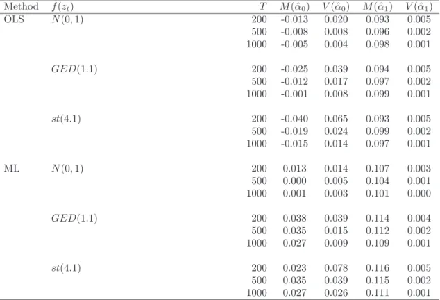
Table 2 contains some simulations that shed light on the finite sample accuracy of some common estimation methods for selected specifications. The finite sample biases are acceptable for many purposes, and estimating the errors {²t} in a
previ-ous step does not seem to affect the estimation precision of α0 and α1 substantially
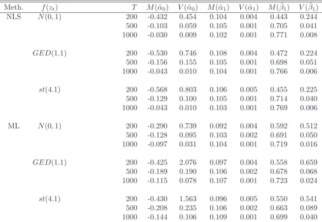
in the second step, or at least not when the persistence in the mean specification is small. Tables 3 and 4 compare least squares estimation via ARMA representa-tions with Gaussian QML estimation (in the standardised errors zt). In table 3
the simulations suggest OLS compares favourably to QML in the estimation of a log-ARCH(1) model, when the standardised errors are more fat-tailed than the nor-mal. When this is the case, then OLS exhibits smaller finite-sample estimation bias of the parameters, and the estimation variances are comparable to or smaller than those of QML. In table 4 the simulations suggest NLS compares well with QML in the estimation of a log-GARCH(1,1) model, when the standardised errors are more fat-tailed than the normal. In this case NLS is more efficient and generally the bias is smaller. The only exception is whenT = 200. So all in all our simulations suggest
NLS via the ARMA representation compares well with QML in finite samples.6
2.5
Inference
In many practical finance applications the mean is either equal to zero or adequately treated as if equal to zero. Or, alternatively, the residuals from the mean specifica-tion are treated as if observable. When this is the case, and when the logarithmic variance specification does not contain log-GARCH terms, then inference regarding the parametersα—apart from the first elementα0—can be undertaken by means of
the usual ordinary least squares theory. When log-GARCH terms enter the power log-variance specification, then a different approach is needed for both the log-ARCH and log-GARCH terms.
Suppose no log-GARCH terms enter the log-variance specification (3), which means (5) reduces to an AR(P) specification withα∗
p =αp. In this case, ifW is the
matrix of observations on the regressors, that is, the first column consists of ones and each row of W is denoted bywt, then the usual test statistic
ˆ
αp
se(ˆαp)
(8)
is approximately N(0,1) in large samples forp= 1, . . . , P under the null ofαp = 0,
where ˆαp is the OLS estimate of the pth. coefficient, and where se(ˆαp) is the pth.
element of the diagonal of the ordinary covariance matrix estimate ˆσ2
u∗
t(W
0W)−1.
The ˆσ2
u∗
t is the standard error of u
∗
t and equal to T−K1
PT
t=1uˆ∗t. In order to conduct
asymptotic inference regarding α0, we may proceed by means of a Wald parameter
restriction test. In the case when the power δ = 2 for example, OLS estimation provides us with the estimate ˆα∗
0. Next, we may testα = 0 by testing whether ˆα∗0 is
equal to −log ˆE[exp(ˆu∗
t)] = −log[T1
PT
t=1exp(ˆu∗t)], since α∗0 = E(logz2t) under the
null of α0 = 0. The Wald-statistic under the null of α = 0 then becomes
{αˆ∗ 0+ log ˆE[exp(ˆu∗t)]}2 d V ar(ˆα∗ 0) asy. ∼ χ2(1), where V ard(ˆα∗
0) is the ordinary coefficient variance estimate of α0∗.
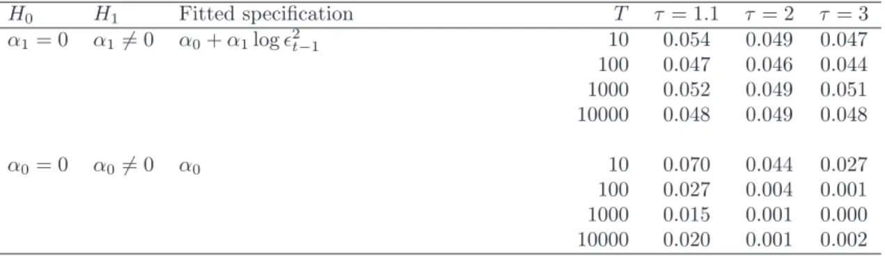
Table 5 contains the simulated finite sample size for two-sided tests of α0 = 0
and α1 = 0 using a nominal size of 5%, and when the power δ = 2. The
simu-lations suggest least squares inference is appropriately sized in finite samples for
α1, since the simulated rejection frequencies range between 4.4% and 5.4% across
density shapes. For the test of α0 = 0, the simulations suggest the Wald test is
un-dersized, since the simulated rejection frequencies are close to 0%. Deviations from
6Our simulations results depend of course on the exact structure of the numerical algorithms
we use. Surely both the NLS and ML algorithms can be improved, so further exploration is needed for a more accurate comparison.
the normal brings the size closer to the nominal, but the discrepancy is nevertheless still notable although acceptable in many practical applications. The undersizedness might suggest that the test lacks power under reasonable departures from the null of
α0 = 0. However, additional simulations (not reported) suggest this is not the case.
Even though the Wald test is undersized under the null, the test carries reasonable power even when the departure from the null is small.
When the logarithmic variance specification contains log-GARCH terms, then one might consider using the usual theory for inference regarding the parameters of the ARMA representation. However, it is doubtful that this theory will be of value in practice, since the AR and MA coefficient estimates will typically be strongly correlated (recall: α∗
p = αp +βp and βq∗ = −βq). An alternative approach is to
conduct inference by means of Wald parameter restriction tests. For example, in log-GARCH(1,1) specifications, one may test whetherα1 = 0 by testing its implication,
namely that α∗
t = (−1)·β1∗, and so on. Another possibility is to use the property
that a {logσδ
t} stationary power log-GARCH specification is (in general) invertible
in the ARMA specification. One may then approximate the log-GARCH part by means of a (possibly long) log-ARCH specification, and next conduct inference on each of the lags. A third approach is to use an information criterion to select between alternative specifications. Finally, one may include a regressor that acts as a local approximation to logσδ
t−1, a “volatility proxy”, and subsequently undertake ordinary
inference on the associated parameter.
2.6
Stochastic volatility
The simplicity of the estimation and inference methods described hitherto are not affected by “stochastic volatility” terms in the power log-variance specification. To see this define
logσδ
t =α0+h(γ, wt) + (logκδ)yt, κ >0, yt∈/xt, (9)
where h(γ, wt) is an abbreviation for the sum of the log-ARCH and log-GARCH
terms, that is, h(γ, wt) =
PP
p=1αplog|²t−p|δ + PQ
q=1βqlogσt−qδ , {yt} is IID and
independent with {zt}, and where the requirementyt ∈/ xt means yt does not enter
the mean equation. It should be noted that, without affecting our argument, yt
can be replaced by yt−1. Indeed, this is needed for {logσδt} to be a Martingale
difference sequence.7 The specification (9) nests many types of stochastic volatility
models, including the autoregressive stochastic volatility (ASV) model of order 1, or ASV(1). Now, denote the information set that does not contain yt for Itsv, and
denote the information set that includes yt for It. If we condition on It, then
consistent estimation via the ARMA representation identifies all the parameters, that is, α0, γ and κ. By contrast, if we condition on Itsv, then σt or volatility is
stochastic. In this case consistent estimation via the ARMA representation does
not identify two parameters, namely α0 and κ, but the others (γ in the example)
are identified. Moreover, the estimate of the conditional variance V ar(rt|Itsv) will
be consistent. To see this recall that
²t = σtzt = exp[α0+h(γ, wt)] 1 δκytzt V ar(rt|It) = σt2 V ar(rt|Itsv) = exp[α0+h(γ, wt)] 2 δE(κ2yt),
assuming the variances exist. Now, the last term can be rewritten asV ar(rt|Itsv) =
exp[˜α0 +h(γ, wt)]
2
δ, where ˜α0 = α0 + logE(κ2yt). In other words, the estimation
procedures described above can be used to estimate ˜α0 andγ, while the standardised
error will now be equal to ˜zt= κytzt
E(κ2yt)12 instead of zt.
2.7
Extensions
Several extensions of the power log-GARCH model suggest themselves. One is the multivariate extension that will be explored in the next section. Another exten-sion, which we do not pursue here, is to specify logσδ
t as a Fractionally Integrated
EGARCH process (FIEGARCH) along the lines of Bollerslev and Mikkelsen (1996). A third type of extension consists simply of adding variables linearly to the logσδ t
specification. This can in many case be done straightforwardly without compro-mising the applicability of the simple estimation and inference methods we have outlined above.
One type of variables that can be added linearly are asymmetry-terms, and in the current context we consider three different types. The first and simplest is of the indicator type I{zt−1<0}, which are equal to 1 when zt−1 < 0 and 0 otherwise.8
In practice this type of asymmetry terms can in general be approximated by means of I²t−1<0, which means the log-GARCH model augmented with such asymmetry
terms can be estimated via an ARMA-X representation. As for stability, the fol-lowing proposition provides quite general sufficient conditions for the existence of the unconditional variance when the standardised errors are either distributed as a student t or as a GED.
Proposition 3. Consider the asymmetricδth. power log-GARCH(1,1) specification logσδ
t =α0+α1log|²t−1|δ+β1logσδt−1+ (logλδ)I{zt−1<0}, 0< λ <∞
8The original economic justification for asymmetry variables is to capture socalled “leverage”
effects in stock markets, see Nelson (1991). So the impact of the regressor is expected to be negative. In some markets, however, for example exchange rate markets, the impact may be either negative or positive depending on which currency is in the denominator of the exchange rate. So we prefer the more general term asymmetry rather than leverage.
with either zt IID∼ GED(τ), τ > 1 or zt IID∼ t(ν), ν > 2. If |α1 +β1| < 1 and if
2α1(α1+β1)i−1 ∈(−1,2] for eachi= 1,2, . . ., then E(²2t)<∞.
Proof. The assumption|α1+β1|<1 means logδt admits the representation α0/(1−
α1 −β1) +
P∞
i=1(α1 +β1)i−1 ·[α1log|zt−i|δ + (logλδ)I{zt−i<0}]. This implies that
(σδ t)2/δ =σt2 = exp[α0δ−1/(1−α1−β1)]· Q∞ i=1(|zt−i|α1λI{zt−i<0})2(α1+β1) i−1 , and that E(²2 t) = exp[α0δ−1/(1−α1−β1)]· Q∞ i=1ai, whereai =E[(|zt−i|α1λ I{zt−i<0})2(α1+β1)i−1]. When λ2(α1+β1)i−1 ∈ (0,1), then λ2(α1+β1)i−1E[|z t−i|2α1(α1+β1) i−1 ] ≤ ai ≤ λ2(α1+β1) i−1 E(|zt−i|2α1(α1+β1) i−1
), and when λ2(α1+β1)i−1 > 1, then E[|z
t−i|2α1(α1+β1) i−1 ] ≤ ai ≤ λ2(α1+β1)i−1E(|z t−i|2α1(α1+β1) i−1
). So each ai will exist |α1+β1|<1 and if 2α1(α1+ β1)i−1 ∈(−1,2]. Finally, since both the two upper bounds and the two lower bounds
will tend to 1 as i→ ∞, thenai →1 and so E(²2t)<∞by means of the same type
of reasoning as in the proof of proposition 2. ¥
Another type of asymmetry-term that can also straightforwardly be included and es-timated via an ARMA-X representation, are asymmetry terms analogous to those of Glosten et al. (1993). In this case the specification of a δth. power log-GARCH(1,1) takes the form
logσtδ =α0 +α1log|²t−1|δ+β1logσδt−1+λlog|²t−1|δI{zt−1<0}.
The exact stability conditions for this specifications are more difficult to derive. Nevertheless, in the case where α1, β1 ≥0 andλ ∈(−1,0), then it follows
straight-forwardly from the results above thatα1+β1 <1 is a sufficient condition for stability.
In particular, the 2nd. moment will exist for student’s tν, ν >2 and GED(τ),τ >1
distributions. The third type of asymmetry-term that can also straightforwardly be included are analogous to those of Nelson (1991). In this case the specification of a
δth. power log-GARCH(1,1) takes the form logσδ
t =α0 +α1log|²t−1|δ+β1logσδt−1+λ²t−1.
However, the stability conditions for this type of specification has not been studied (but see Dahl and Iglesias (2008) where {²t} is assumed strictly stationary and
ergodic). Also, it is not clear that the results and methods above are applicable, since least squares and maximum likelihood methods may not provide consistent estimates of an ARMA-X representation.
A second type of variables of special interest that can be added linearly are volatility proxies. For example, if Vδ
t is a volatility proxy in the δth. power, then
a diagnostic tool of the volatility proxy that naturally suggests itself is a logarith-mic version of Mincer and Zarnowitz (1969) regressions. In logarithlogarith-mic versions of Mincer-Zarnowitz regressions the log-variance logσδ
t is equal to γ0+γ1logVtδ, and
the joint test γ0 = 0 and γ1 = 1 is a test of whether Vtδ is an “unbiased” estimate
of σδ
t. Moreover, adding variables to the Mincer-Zarnowitz specification readily
per-mits encompassing tests of Vδ
whether Vδ
t parsimoniously encompasses the other candidate variables (log-ARCH
terms, log-GARCH terms, volume variables, etc.). Then this can simply be done in terms of a joint hypothesis test framework of a general specification that nest the variables. A volatility proxy of particular interest is the lag of the equally weighted moving average (EWMA) of past squared errors (EW MAt−1). The EWMA is very
simple to compute and is always available since it does not require the acquisition of high-frequency data like (say) realised volatility (RV).9 Also, the EWMA often
performs well in practice when compared with many of its technically more sophis-ticated competitors.
3
A multivariate power log-GARCH model
Financial markets tend to move together, and the extent to which they do so varies over time. This is the main motivation behind multivariate ARCH models, and the implications for asset pricing was the original context in which Bollerslev, En-gle and Wooldridge (1988) first proposed a multivariate ARCH moel, see Bauwens et al. (2006) for a recent surveys. For the power log-GARCH class of models, there exists a straightforward multivariate generalisation of the univariate class that can be estimated by means of common methods via its vector ARMA (VARMA) repre-sentation. This multivariate version is not simply a collection of univariate power log-GARCH models. Indeed, the model is truly multivariate in that P log-ARCH terms of each of the M variables enter each of the M equations, and in that Q
log-GARCH terms enter in each of the M equations.
3.1
Notation and specification
Suppose {²t} is a sequence of (M × 1) vectors of mean errors. Then the M
-dimensional power log-GARCH(P, Q) model is given by
²t= diag(σt)zt, zt|It∼IID(0, Cov(zt)), V ar(zt|It) =IM, (10)
where σt is the (M ×1) vector of conditional standard deviations, diag(σt) is an
(M ×M) diagonal matrix with σt on the diagonal and zeros elsewhere, zt is the
(M ×1) vector of standardised errors, Cov(zt) is the variance-covariance matrix of
{zt}, and It is the conditioning set in question. Here, It ={zt−1, zt−2, . . .}. At this
point it is worth noting that we do not impose any restrictions on the off-diagonal entries ofCov(zt). In other words, the covariances ofzt may not be positive definite
(we will return to this issue below in subection 3.3). TheM-dimensional log-variance
9The P periodEW M A
t−1 is equivalent to an integrated ARCH(P) model with the variance
specification is given by logσδ t = α0+ P X p=1 αplog|²t−p|δ+ Q X q=1 βqlogσt−qδ , P ≥Q, (11) where logσδ t = logσδ 1,t ... logσδ m,t ... logσδ M,t , α0 = α1,0 ... αm,0 ... αM,0 , αp = α11.p · · · α1m.p · · · α1M.p ... . .. ... ... αm1.p · · · αmm.p · · · αmM.p ... ... . .. ... α11.p · · · α1m.p · · · α1M.p , log|²t−p|δ = log|²1,t−p|δ ... log|²m,t−p|δ ... log|²M,t−p|δ , βq = β11.q · · · β1m.q · · · β1M.q ... . .. ... ... βm1.q · · · βmm.q · · · βmM.q ... ... . .. ... βM1.q · · · βM m.q · · · βM M.q .
For example, the specification of a two-dimensionalδth. power log-ARCH(1) model is
logσ1δ,t = α1,0+α11.1log|²1,t−1|δ+α12.1log|²2,t−1|δ
logσδ
2,t = α2,0+α21.1log|²1,t−1|δ+α22.1log|²2,t−1|δ,
whereas the specification of a two-dimensional δth. power log-GARCH(2,1) is logσδ
1,t = α1,0+α11.1log|²1,t−1|δ+α12.1log|²2,t−1|δ+α11.2log|²2,t−2|δ
+α12.2log|²2,t−2|δ+β11,1logσδ1,t−1+β12,1logσδ2,t−1
logσδ
2,t = α2,0+α21.1log|²1,t−1|δ+α22.1log|²2,t−1|δ+α21.2log|²2,t−2|δ
+α22.2log|²2,t−1|δ+β21,1logσδ1,t−1+β22,1logσδ2,t−1,
and so on.
The following proposition provides a general set of non-restrictive sufficient con-ditions for the existence of the unconditional moments.
Proposition 4. Consider an M-dimensional δth. power log-GARCH(P, Q) model with P ≥ Q that admits the representation logσδ
t = Ψ0 +
P∞
i=1Ψilog|zt−i|δ with
{Ψi} being an absolutely summable sequence of (M ×M) matrices. Then the sth.
unconditional moment E(²s
m,t) = exp(sδ−1ψm,0)·
Q∞
i=1E £
|z1,t−i|sψi,m1|z2,t−i|sψi,m2· · ·
|zM,t−i|sψi,mM
¤
, s ∈ {1,2, . . .}, of variable m ∈ {1, . . . , M} exists if E£|z1,t−i|sψi,m1
|z2,t−i|sψi,m2· · · |zM,t−i|sψi,mM
¤
Proof. By definition, absolute summability of the matrix sequence {Ψi} means
P∞
i=1|ψi,mn| < ∞ for each m, n ∈ {1,2, . . . , M}. Next, a sufficient condition
for an infinite product Q∞i=1ai to converge to a finite, nonzero number is that
the series P∞i=1|ai − 1| converges (Gradshteyn and Ryzhik (2007, section 0.25)).
Since E£|z1,t−i|sψi,m1|z2,t−i|sψi,m2· · · |zM,t−i|sψi,mM
¤
→ 1 as i → ∞ due to abso-lute summability, it follows that |ai −1| → 0 as i → ∞. Accordingly, if ai =
E£|z1,t−i|sψi,m1|z2,t−i|sψi,m2· · · |zM,t−i|sψi,mM
¤
< ∞ for each i, it follows that E(²s mt)
exists. ¥
In practice, the natural condition to check is whether all the eigenvalues of the (M ×M) matrix PpP=1∗ (αp +βp) are smaller than 1 in modulus. If this is the case,
then{Ψi}is absolutely summable. Whether the second condition is satisfied or not,
that is, E£|z1,t−i|sψi,m1|z2,t−i|sψi,m2· · · |zM,t−i|sψi,mM
¤
< ∞ for each i, will depend on the distribution of zt.
3.2
VAR and VARMA representations
The parameters of the power log-GARCH(P, Q) model can be consistently estimated by means of common methods via its VARMA representation subject to appropriate assumptions. Specifically, the VAR(P) representation of an M-dimensional power log-ARCH(P) model is given by
log|²t|δ = α∗0+
P
X
p=1
αplog|²t−p|δ+u∗t, (12)
where αp is defined as above, and where
log|²t|δ = log|²1,t|δ ... log|²m,t|δ ... log|²M,t|δ , α∗ 0 = α1,0+ logE|z1,t|δ+E(log|z1∗,t|δ) ... αm,0+ logE|zm,t|δ+E(log|zm,t∗ |δ) ... αM,0+ logE|zM,t|δ+E(log|z∗M,t|δ) u∗ t = log|z∗ 1,t|δ−E(log|z1∗,t|δ) ... log|z∗ m,t|δ−E(log|zm,t∗ |δ) ... log|z∗ M,t|δ−E(log|zM,t∗ |δ) . In other words, {u∗
t} is now a vector zero-mean IID process. The VARMA(P, Q)
representation of an M-dimensional power log-GARCH(P, Q) model is given by
log|²t|δ = α∗0+ P X p=1 α∗plog|²t−p|δ+ Q X q=1 βq∗u∗t−q+u∗t, (13)
where
αp∗ =αp+βp, βq∗ =−βq, α∗0 =α0+(IM−
Q
X
q=1
diag(βq))[logE|zt|δ+E(log|zt∗|δ)],
α0 = α1,0 ... αm,0 ... αM,0 , logE|zt|δ+E(log|zt∗|δ) = logE|z1,t|δ+E(log|z1∗,t|δ) ... logE|zm,t|δ+E(log|zm,t∗ |δ) ... logE|zM,t|δ+E(log|zM,t∗ |δ) .
As in the univariate case, if P > Q then βQ+1 = · · ·=βP = 0 by assumption, and
the formulas in proposition 1 can be used to estimate logE|zt|δandE(log|zt∗|δ) once
the VARMA representation has been estimated.
In theory, multivariate δth. power log-GARCH models can be consistently esti-mated by means of common estimation methods (say, least squares or QML) via its VARMA representation. However, it is well known that, in practice, VARMA mod-els may not be readily estimated due to numerical issues. The question of how well the available estimation estimation algorithms actually work for the multivariate log-GARCH we leave for future research.
3.3
Modelling conditional covariances
A key motivation for multivariate GARCH models is that they can be used in the computation of portfolio variances. However, unless restrictions are imposed on the off-diagonals of the covariance matrix Ht = Cov(²t), then one cannot be
ensured that such portfolio variances will be positive. This is the motivation for the socalled positive definiteness requirement of Ht. In the power log-GARCH model
this amounts to positive definiteness of Cov(zt). The methods we have outlined so
far do not rely on any specific property on the covariance-matrix of {zt}. Indeed,
the only assumption we rely upon is that V ar(zt) = IM. Our estimation methods
are thus compatible with Cov(zt) being positive definite or not.
4
Empirical applications
One type of problems that specifications in the power log-GARCH class of models might be particularly suited for are those that involves many explanatory variables. Indeed, specifications contained in the 2nd. power log-GARCH-X class have proved useful in explanatory exchange rate modelling and forecasting, in stock price volatil-ity proxy evaluation, and in value-at-risk portfolio forecasting, see Bauwens et al. (2006), Rime and Sucarrat (2007), Bauwens and Sucarrat (2008), and Sucarrat and
Escribano (2009). Here we explore further the usefulness of power log-GARCH mod-els in three empirical applications. The first two are devoted to the univariate and multivariate analysis of stock market variability. This choice is motivated by the fact that the modelling and forecasting of stock market variability is one of the more frequent use of GARCH models. The third empirical application applies the power log-GARCH model to the complex problem of modelling daily electricity prices. The relative change in daily electricity prices differ from most other financial returns in that they exhibit strong and complex patterns of autoregressive persistence and periodicity, both in the mean and volatility specifications.
4.1
Log-ARCH models vs. the GARCH(1,1)
In the ARCH class of models introduced by Engle (1982), the GARCH(1,1) specifica-tion of Bollerslev (1986) is possibly the most common model of financial variability. In this subsection we therefore compare the GARCH(1,1) with four simple models of the power log-ARCH class in modelling SP500 variability both in-sample and out-of-sample. We choose the SP500 stock market index because it is widely used for the purpose of comparison.
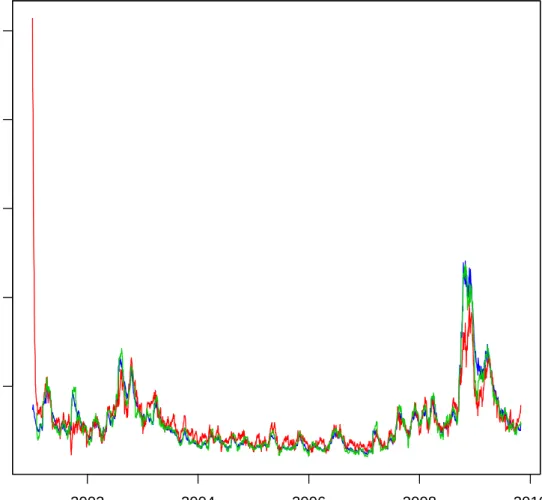
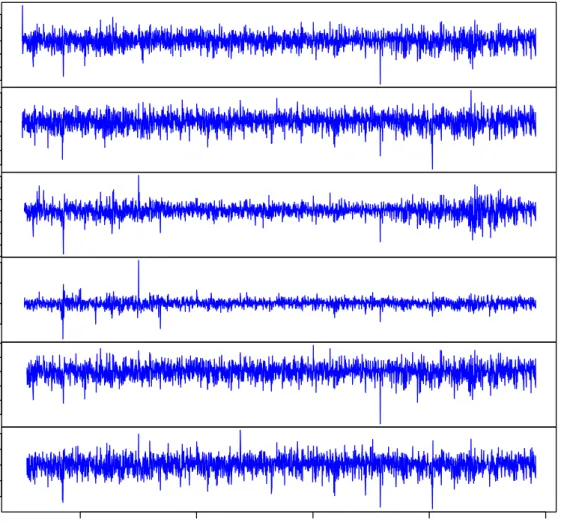
Our estimation sample is 1 January 2001 - 31 December 2005 (1305 observations), whereas our out-of-sample evaluation period is 1 January 2006 - 30 October 2009 (997 observations).10 The ARCH models are all fitted to the “demeaned” log-returns
in percent (see figure 1), where the mean is an OLS estimated AR(1) specification equal to rt = φ0 +φ1rt−1 +²t. The same mean specification is used out-of-sample
to demean the returns. The estimation results of the GARCH(1,1) specification, a 2nd. power log-GARCH(1,1) specification, a 1st. power log-GARCH(1,1) specifica-tion, a 2nd. power log-ARCH(1) specification augmented with the log of a 20-day11
equally weighted moving average (EWMA(20)t−1) of past squared residuals as
re-gressor, that is, a volatility proxy, and a 2nd. power log-ARCH(0) specification with
logEW MA(20)t−1 as only regressor, are12
ˆ
σ2
t = 0.006 + 0.061ˆ²2t−1+ 0.934ˆσt−2 1 (14)
10The source of the raw series is Reuters-EcoWin Pro, and the series identifier is ew:usa15510200.
1120 trading days corresponds in general to 4 weeks or approximately one calendar month.
12AR
1 is the 1st. order serial correlation of {zˆt}, whereas ARCH1, ARCH2 and ARCH5 are
the 1th., 2nd. and 5th. order serial correlations of{zˆ2
t}. The values in square brackets arep-values
from Ljung and Box (1979) tests of no serial correlation up to the lag order in question. JB is
the Jarque and Bera (1980) test statistic with the associated p-value in square brackets. V ar is
the sample variance of the standardised residuals {zˆt}. The GARCH(1,1) model is estimated by
means of QML using the garch() function in the tseries R package, see Trapletti and Hornik
(2009). The log-GARCH(1,1) model is estimated by means of NLS via the ARMA representation
using thearma()function, which is also part of thetseries R package. The volatility proxy model
AR1 ARCH1 ARCH2 ARCH5 JB V ar {zˆt} in-sample: −0.04 [0.17] −[00.12].04 [00..0221] 0[0..0230] [023.00] 1.00 {zˆt} out-of-sample: −0.10 [0.00] −[00.16].04 −[00.35].01 0[0..0273] [0355.00] 1.10 log ˆσ2 t = 0.091 + 0.0533 log ˆ²2t−1+ 0.9242 log ˆσt−2 1 (15)
AR1 ARCH1 ARCH2 ARCH5 JB V ar
{zˆt} in-sample: 0.00
[0.99] 0[0..0168] [00..0605] 0[0..1200] [08.K00] 0.99
{zˆt} out-of-sample: −0.11
[0.00] −[00.84].01 [00..0442] 0[0..1001] [0237.00] 1.17
log ˆσt = 0.045 + 0.0532 log|²ˆt−1|+ 0.9243 log ˆσt−1 (16)
AR1 ARCH1 ARCH2 ARCH5 JB V ar
{zˆt} in-sample: 0.00
[0.99] 0[0..0168] [00..0705] 0[0..1200] [08.K00] 0.99
{zˆt} out-of-sample: −0.11
[0.00] −[00.84].01 [00..0442] 0[0..1001] [0237.00] 1.17
log ˆσ2t = 0.100 + 0.005 log ˆ²t−2 1+ 0.901 logEW MA\ (20)t−1 (17)
AR1 ARCH1 ARCH2 ARCH5 JB V ar
{zˆt} in-sample: −0.04
[0.14] −[00.12].04 [00..0320] 0[0..0220] [018.00] 1.00
{zˆt} out-of-sample: −0.10
[0.00] −[00.23].04 −[00.44].02 0[0..0184] [0430.00] 1.12
log ˆσt2 = 0.089 + 0.906 logEW M A\ (20)t−1 (18)
AR1 ARCH1 ARCH2 ARCH5 JB V ar
{zˆt} in-sample: −0.04
[0.13] −[00.18].04 [00..0325] 0[0..0221] [015.00] 1.00
{zˆt} out-of-sample: −0.10
[0.00] −[00.26].04 −[00.47].02 0[0..0186] [0425.00] 1.12
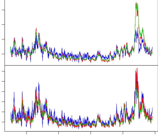
Figure 1 graphs the demeaned residuals, whereas figures 2-3 contain graphs of the associated in-sample and out-of-sample standard deviations and standardised resid-uals, respectively. It should be noted that the standard deviations and the standard-ised residuals of the 1st. and 2nd. power log-GARCH(1,1) models are indistinguish-able from each other graphically, and similarly for the 4th. and 5th. models. The reason why the 1st. and 2nd. power log-GARCH(1,1) models’ are so similar is pre-sumably that the variance constant α0 in both log-GARCH(1,1) specifications are
close to zero. Whenα0 is exactly equal to zero, then allδth. power log-GARCH(1,1)
models are equivalent. This can be seen by studying the effect of changing δ in the ARMA representation (5), and in the autocorrelation structure of {²2
t}(see the
term explain very little of the time-varying volatility compared with the volatility proxy.
Additionally, there are at least five more features worth noticing from the es-timation results of equations (14)-(18), and from the figures. First, the estimates
ˆ
α0,αˆ1 and ˆβ1 of the log-GARCH(1,1) specifications are relatively similar to those of
the GARCH(1,1), and the sum ˆα1 + ˆβ1 is close to (but below) 1 in all three cases.
Second, from the figures it is clear that the fitted conditional standard deviations are relatively similar. The greatest difference is that the two log-GARCH(1,1) spec-ifications (standard deviations in red) seem to generate lower standard deviations in high variability periods (towards the end of 2008). A third feature of interest is that the estimation results above suggest all the models appear to be relatively (parameter) stable across the two periods. This interpretation is due to the sample variancesV ar(ˆzt) being relatively close to 1 out-of-sample. Fourth, theJB-statistics
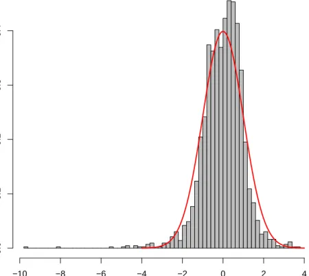
in the results above, and the figure with the standardised residuals, suggest the log-GARCH(1,1) specifications generate standardised residuals that are more fat-tailed than those of the first and last two models. Finally, the ARCH diagnostic tests in the results above do not suggest the log-GARCH(1,1) specifications depict the ARCH in SP500 variability as well as the other models both in and out-of-sample.
4.2
Multivariate ARCH models
In this subsection we compare four joint models of the daily S&P500 and the FTSE Euro 100 (EUR100) stock market index returns from 1 January 2001 to 30 October 2009.13 The S&P500 return series is the same demeaned series as in the previous
subsection, and we use the same approach in demeaning the EUR100 returns. Both demeaned series are displayed in figure 1. Also, we repeat the exercise of using the data up to and including 2005 in estimating the models, and then generating out-of-sample conditional variances, standardised residuals, etc., from the beginning of 2006 until 30 October 2009.
The first of the three models we fit is a diagonal BEKK(1,1,1) model estimated by means of multivariate Gaussian ML.14 The second model is a two dimensional 2nd.
power log-GARCH(1,1) model, which we estimate by means of two-stage equation-by-equation OLS via the VARMA representation. (In the first OLS step we set the common lag-length in the VAR representation as equal to the natural logarithm of the sample size, see Kascha (2007) for a comparison of various VARMA estimation methods, including ours.) The third is a four dimensional 2nd. power log-ARCH(1) model augmented with volatility proxy dynamics (we use the same method as in the
13The source of the EUR100 series is also Reuters-EcoWin Pro, and its series identifier is
ew:emu15555.
14This model we estimate with the OxMetrics package G@RCH 5.1, see Laurent (2007). We
only report the estimation results of the diagonal of the covariance matrix Ht, and the estimates
are reported in their GARCH(1,1) form. For example, in the first equation, the estimate 0.01 is
equal toc2