Nonlinear manifold learning for model reduction in finite elastodynamics

Nonlinear manifold learning for model reduction in finite elastodynamics

Daniel Mill´anI_{and Marino Arroyo}⇤

Dept. Applied Mathematics 3, LaC`aN, Universitat Polit`ecnica de Catalunya-BarcelonaTech, Barcelona 08034, Spain

Abstract

Model reduction in computational mechanics is generally addressed with linear dimensionality reduction methods such as Principal Components Analysis (PCA). Hypothesizing that in many applications of interest the essential dynamics evolve on a nonlinear manifold, we explore here reduced order modeling based on nonlinear dimen-sionality reduction methods. Such methods are gaining popularity in diverse fields of science and technology, such as machine perception or molecular simulation. We consider finite deformation elastodynamics as a model problem, and identify the manifold where the dynamics essentially take place –the slow manifold– by nonlinear dimensionality reduction methods applied to a database of snapshots. Contrary to linear dimensionality reduction, the smooth parametrization of the slow manifold needs special techniques, and we use local maximum entropy approximants. We then formulate the Lagrangian mechanics on these data-based generalized coordinates, and de-velop variational time-integrators. Our proof-of-concept example shows that a few nonlinear collective variables provide similar accuracy to tens of PCA modes, suggesting that the proposed method may be very attractive in control or optimization applications. Furthermore, the reduced number of variables brings insight into the me-chanics of the system under scrutiny. Our simulations also highlight the need of modeling the net e↵ect of the disregarded degrees of freedom on the reduced dynamics at long times.

Keywords: Reduced order modeling, nonlinear dimensionality reduction, finite deformation elastodynamics, maximum entropy approximants, variational integrators

1. Introduction

The goal of model reduction is to process (simulate, control, optimize) a complex system in terms of a much simpler description. The premise is that, with a proper selection of the reduced model, the essential features of the original system can be preserved by a very light and efficient model. Most often, the reduced model is constrained to evolve in an affine subset of the full configuration space, for instance when a large finite element model is reduced by means of a linear combination of modes selected by proper orthogonal decomposition (POD). Such approaches are common in electrical engineering, molecular simulation, or mechanics [1], and recent applications include real-time simulation [2]. The termnonlinear model reductiongenerally refers to the reduced modeling of a nonlinear system, yet relying on a linear (affine) reduced description [3,4]. Nevertheless, it is apparent that many models evolve on essentially nonlinear manifolds, in particular those involving large amplitude rotations or steric constraints. Rotations, prominent in many mechanical systems, are the paradigmatic example of a nonlinear motion inefficiently described by a linear geometric model. For instance, in three dimensions, nine Cartesian components are required to describe an orthogonal matrix, while only three parameters, e.g. Euler angles, suffice to parametrize a rotation.

In the field of statistical learning and pattern recognition, there has been a very intense research activity over the last decade in nonlinear dimensionality reduction (NLDR) of data sets [5]. These techniques extend the classical ideas of multi-dimensional scaling (MDS) or principal component analysis (PCA) to detect nonlinear hidden correlations in data lying in high dimensional spaces. These methods provide low-dimensional embeddings of the data, often shedding light on very complex phenomena. These methods have found applications in classification, automatic perception, climate science [6], the study of the conformation dynamics of molecules [7,8], or galaxy spectra classification [9]. We have exploited elsewhere these methods for the meshfree thin shell analysis [10], and to analyze the stroke kinematics of a micro-organism [11].

I_{Current address: Laborat´orio Nacional de Computac¸˜ao Cient´ıfica, Petr´opolis, RJ, Brazil} ⇤_{Correspondence to: [email protected]}

Here, we explore the application of NLDR techniques to the reduced modeling of mechanical systems. In this first study, we restrict ourselves to conservative mechanical systems, and to the forward problem. We fol-low the classical method of snapshots, in which a training set of simulations, representative of the behavior of the system, is used as the basis for the reduced model. Unlike linear approaches such as the POD (a direct ap-plication of PCA), here we consider a nonlinear reduced description, and consequently cannot parametrize the reduced model as a linear combination of modes. We proceed in three steps. First, the snapshots are viewed as a high-dimensional ensemble representative of the configurations of the system, the intrinsic dimensionality of the underlying slow manifold is detected, and the snapshots are embedded in low-dimensions by NLDR. Note that a mere low-dimensional embedding of the snapshots is not enough for our purpose, as it does not provide a parametrization of the slow manifold. For this reason, as a second step, we construct a smooth parametrization of the slow manifold (a map from the low-dimensional embedding to high dimensions) with local maximum-entropy (LME) approximants [12]. A number of key features of this approximation method are essential for the generality and success of the proposed method, namely its ability to provide smooth approximations from scattered unstruc-tured data in any spacial dimension (a typical output of NLDR), and to filter noisy data robustly. As the third step, the embedding dimensions are viewed as generalized coordinates of the system, in terms of which we express the dynamics. Although the real system evolves in a high dimensional space and departs from the slow manifold during its dynamics, we constrain the dynamics of the reduced system to the slow manifold.

There have been extensions beyond linear representations of reduced models, `a la PCA, in computational mechanics. For instance, proper generalized decomposition methods [13] address high-dimensional problems by finding iteratively new basis functions of separated variables, resulting in a nonlinear approximation method. Farhat and co-workers have proposed methods to interpolate parametrized reduced models, which form a nonlinear manifold [14].

The present work is organized as follows. Section2describes our model system, nonlinear elastodynamics, and succinctly its space discretization. Section3outlines the methodology proposed here. We formulate in Section

4 the Lagrangian mechanics of a system constrained to evolve in a manifold described by a set of generalized coordinates. We exercise the discrete Lagrangian mechanics formalism to derive variational time-integration schemes for systems with configuration-dependent mass. In Section5, we develop a proof-of-concept example, highlighting the potential and limitations of reduced order modeling based on NLDR. Finally, we put forward some remarks and conclusions in Section6.

2. Model system: nonlinear elastodynamics

We consider nonlinear elastodynamics as a model system to illustrate the proposed nonlinear model reduction method. Given the undeformed elastic body⌦₀⇢Rn, wherenis the spatial dimension of the problem, subject to body forces, with prescribed deformation on part of its boundary@⌦D₀, and prescribed tractions in the rest of the boundary of the body@⌦N₀, the goal is to obtain the deformation mapping': ⌦₀ ! Rn satisfying balance of linear momentum and the boundary conditions:

⇢0'¨ DivP ⇢0b=0 in⌦0

'=' on@⌦D₀

P N =t on@⌦₀N,

(1) with initial conditions '_|t=0 ='¯0, and ˙'|t=0='˙¯0in⌦0. Here Div denotes the divergence in material coordinates, P is the first Piola-Kirchho↵ stress tensor, b the body force per unit mass, N the unit outward normal to the boundary of the undeformed body,tis the prescribed traction per unit undeformed area,⇢0is the mass density in

the reference configuration, and'is the prescribed deformation mapping in part of the boundary. These equations

need to be supplemented by the constitutive relation, which in hyper-elastic materials takes the form P(X)= @W

@F D'(X), 8X2⌦0. (2)

HereW(F) is the free energy density of the material, whose argument is the deformation gradient, i.e. the derivative of the deformation mappingF =D'. For definiteness, we consider here a compressible neo-Hookean material with strain-energy density

W(F)= 1 2 ln2(J)+ 1 2µ ⇣ tr(FT_{F) n}⌘ _{µln(J), (3)}

The standard finite element discretization of this problem relies on the weak form of these equations and the finite element interpolation of the deformation mapping and the test functions. Alternatively, the discrete equations of motions can be derived following a Lagrangian formalism, by discretizing directly the kinetic and the potential energies. The total potential energy of the system is

V[']= Z ⌦0 W(D')dV Z ⌦0 ⇢0b·'dV Z @⌦N₀ t·'dS, (4)

whereas the kinetic energy is

T[ ˙']=1 2

Z

⌦0

⇢0'˙·'˙dV. (5)

In the finite element approximation, the deformation mapping is discretized as

'h(X,t)=

X i

'i(t)Ni(X), (6)

where'idenote the nodal positions andNi(X) are the basis functions defined in the undeformed body.

Conse-quently, the Lagrangian velocity field is ˙ 'h(X,t)= X i ˙ 'i(t)Ni(X). (7)

We denote by x =('1,'2, . . .) 2 RDthe array containing all the nodal positions. Plugging Eqs. (6,7) into the

potential and kinetic energy functionals, we obtain the discrete potential and kinetic energy functionsVh(x) =

V['h] andTh( ˙x) =T[ ˙'h], which also involve numerical quadrature. The out-of-balance forces at nodebcan be

computed with the usual expression

@Vh @'b = Z ⌦0 Pr0NbdV Z ⌦0 Nb⇢0b dV Z @⌦N₀ Nbt dS, (8)

wherer0is the gradient with respect to the reference coordinates. The kinetic energy adopts the simple expression

Th( ˙x)= 1

2x˙TMx˙, (9)

where the mass matrix components are

Maib j= i j Z

⌦0

⇢0NaNbdV. (10)

3. Point-set manifold analysis

We concisely describe here the main steps required to describe the data-driven slow manifoldM, namely (1) the computation of a low-dimensional embedding of a training set of snapshots, and (2) the definition of a smooth parametrization of the slow manifold embedded in high dimensions. Before performing NLDR, the training set needs some preprocessing, described in Section3.1, and the intrinsic dimension of the datadcan be estimated by various techniques for a better-targeted reduction, Section3.2. Dimensionality reduction is described in Section

3.3, and the parametrization of the slow manifold in Section3.4. 3.1. Preparing the training ensemble

We assume now that, on the basis of an o✏ine set of calculations, we have a configuration ensemble made out of simulation snapshots. In practice, a decimation step is necessary to define a workable training set, which we denote byX = {x₁,x2, . . . ,xN} ⇢ RD. We define the ensemble such that any two snapshots are at least a

cut-o↵distance away from each other, following a standard procedure in neural network analysis known as vector quantization [5], although many other more sophisticated techniques are available.

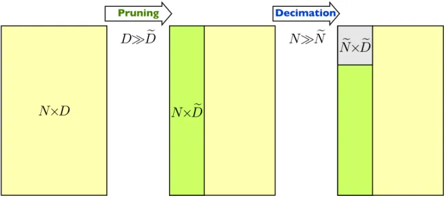
Unlike PCA, which requires the snapshots to be full vectors inRD_{to avoid a lossy compression of the data,}

see Eq. (11) below, the method presented here allows us to prune the snapshots into coarser representations which retain the main features before applying NLDR, see Fig.1. With the parametrization of the slow manifold de-scribed in Section3.4, such pruning step does not require specialized techniques for gappy data typical of linear methods [15] to reconstruct full configurations. For instance, it is easy to simplify a large finite element mesh to

a set of landmark points sampling the boundary, edges, or the skeleton (see [16] for a systematic method), and thus decreaseDsignificantly. This allows us to circumvent the manipulation and storage of large amounts of data. For instance, with a 3D mesh with 10000 nodes and 105_{snapshots, the unpruned training set requires about 22}

GB of memory. We view pruning as problem-dependent, and strongly relying on experience and intuition. For the problem at hand, we have found that the embeddings resulting from full conformations are very close to those resulting from pruned conformations given by the boundary nodes.

Pruning Decimation

N D

N D

D D

N D

N N

Figure 1: Sketch illustrating the pruning and decimation procedures to reduce the memory requirements and computing time of NLDR. The box in the left represents the original training set containingNfull configurations of dimensionD. Prior to applying NLDR to the high-dimensional data, the high-dimensionality can be reduced by adopting a simplified representation of the configurations, e.g. keeping the nodes at the boundary of the body resulting in a dimensionDe⌧ D. We refer to this as the pruning step. Furthermore, a large training set can be significantly reduced without loosing significant information by decimation, which retains fewer configurations representative of neighboring states.

3.2. Intrinsic dimension

In PCA, the decay of the spectrum of the covariance matrix provides valuable information about the dimension of the affine hull of the data. Nonlinear dimensionality reduction methods require guessing the intrinsic dimension dof the underlying nonlinear manifoldM, a much more difficult task. The notion of intrinsic dimension is not clear-cut, and for data infected by noise, a generic situation, it depends on the scale of observation. It can be loosely defined as the minimum number of variables needed to describe the system behavior within a confidence level. The dimension can be estimateda priori, or the appropriateness of a guess can be assesseda posteriori.

A number of methods have been proposed to estimated. We consider here the correlation dimension of the full data setX, which estimates the dimension by tracking the growth of the number of samples within a ball of increasing radius, and local PCA, in which the affine dimension is estimated for patches ofX of a certain size located at di↵erent positions, as locally a manifold should look linear. The interested reader is referred to [5], and references therein. We discuss in Section3.5thea posteriorievaluation of the dimension.

3.3. Dimensionality reduction

We describe now how to embed the training setX⇢RD_{in dimensiond, i.e. find a reduced representation of}

the snapshotsQ=_{q₁,q2, . . . ,qN}⇢Rdby dimensionality reduction methods. Dimensionality reduction tries to

reduce the redundancy of high-dimensional data sets by identifying correlations hidden in the data. This is done by finding a lowerd dimensional representation,d ⌧D, which captures the most relevant features of the data. In other words, these methods identify the hidden variables, which best explain the behavior of a given system. The most widely used methods seek for linear correlations between the high-dimensional coordinates, resulting in affine slow manifolds. However, over the last decade, there has been an intense research activity in nonlinear dimensionality reduction [17,18], originating from the observation that many high-dimensional systems display strongly nonlinear correlations, which when properly identified, lead to extremely low-dimensional representa-tions. This research has had a profound impact in many scientific disciplines. The interested reader is refereed to [5] and references therein.

Linear Model Reduction. PCA is a classical linear dimensionality reduction method [19], widely used in model order reduction, e.g. by [1] in the context of nonlinear solid dynamics. First, the spectral decomposition of the

covariance matrix, aD⇥Dmatrix, is computed, or more conveniently the singular value decomposition of the centered snapshot matrix. Then, a matrix with the eigenvectors associated to thedlargest eigenvalues,P2RD⇥d_,

is defined. The low-dimensional embedding is computed through the projection qa = PT(xa x), where ¯¯ x =

PN

a=1xa/N. Note that this projection can be applied to out-of-sample high dimensional points, i.e. points not belonging to the training setX. Conversely, PCA provides a direct parametrization of the slow manifold (an affine subset ofRD_{) as}

X(q)=Pq+x¯, ₈q2Rd_{. (11)}

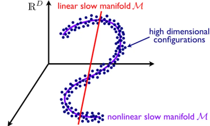
Figure2illustrates how PCA approximates the data with thed dimensional affine manifold that best describes the variance. However, if the data lies on a curved manifold, PCA provides in general a poor description unless a dimension larger than the intrinsic dimension is considered. However, if dimension is increased, the reduced description becomes inefficient and does not reveal the nature of the system.

Multi-dimensional scaling (MDS) provides a complementary point of view to PCA. The low-dimensional embedding is found by minimizing the discrepancy between the distance matrix of the points in low dimensions and the distance matrix in high-dimensional space. If the distance metric is Euclidean, this method coincides with PCA. However, it involves the spectral decomposition of aN⇥Nfull matrix, which can be beneficial or not depending on the application.

nonlinear slow manifold

high dimensional configurations

R

_M

M

Wednesday, 4 July 12

Figure 2: Sketch of the the slow manifold obtained with linear and nonlinear dimensionality reduction methods from a data set with low-dimensional nonlinear correlations (dark blue points). A linear method (red line) only captures the variability if the number of dimensions is larger than the intrinsic dimension, hered=1, whereas the nonlinear method, at the expense of extra complexity, can describe the system

optimally in terms of dimensionality. Note that NLDR algorithms do not provide a description of the nonlinear slow manifold (purple line), but only a low-dimensional embedding, see Fig.4.

Nonlinear Model Reduction. Nonlinear dimensionality reduction or manifold learning methods try to identify automatically nonlinear, low-dimensional correlations in the high-dimensional data. In this category there exists a myriad of techniques that can be split in two major groups, as direct and iterative methods. Another way to classify such methods is between metric and non-metric methods. Since nonlinear dimensionality reduction methods are often used to classify or visualize high-dimensional data, preserving relative distances of the high-dimensional points in the low-dimensional embedding is not essential. In fact, important methods in the field such as Locally Linear Embedding [18] ignore metric information. However, in the present context we prefer to focus on methods that try to preserve metric information. With such methods, the low-dimensional embedding of the data points inherits to some degree the isotropy and uniformity of the original high-dimensional sampling. They also lead to more regular parametrizations of the slow manifold, as defined in the next subsection.

One of the most popular direct methods, Isomap [17], tries to isometrically embed the high-dimensional data inRd_{through MDS. The key point is that the distance matrix of the points inXis an approximation to the geodesic}

distance, not the Euclidean distance. Therefore, the embedding tries to respect distances on the low-dimensional manifold, not Euclidean distances in high-dimensions. The approximation to the geodesic distance between two snapshots is the shortest path in a graph built from the nearest-neighbor connections between snapshots based on their high-dimensional Euclidean distance, since locally a manifold behaves as Euclidean space. Isomap has been shown to be robust for data polluted with noise, or for non-uniformly distributed data points. However, even for surfaces in three dimensions, we know as a corollary of Gauss’s Theorema Egregium [20] that it is not possible to isometrically embed inR2_{a surface with non-zero Gaussian curvature. This fact leads to a frustration}

in the algorithm when handling highly curved manifolds, which can lead to instabilities and generate collapsed low-dimensional embeddings. As we shown in Section5, this spurious behavior manifests itself in practical appli-cations, and demands more robust methods. It can be dealt with by partitioning the training set into geometrically

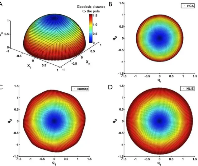
Geodesic distance to the pole

A

B

C

D

Figure 3: Dimensionality reduction example fromD =3 tod =2. (A) Scattered set of points uniformly sampling a hemisphere.

Two-dimensional embeddings obtained by (B) PCA, (C) Isomap and (D) NLIE. The metric distortions introduced by PCA and Isomap are apparent. The colormap indicates the geodesic distance from the pole in the top of the hemisphere to a given point on the surface.

simpler pieces. Partitioning is also necessary when dealing with manifolds of complex topology. We have dis-cussed these issues in [10], where each partition of the data corresponds to a chart of an atlas of the complete manifold, and the di↵erent charts are stitched with a partition of unity.

To deal with the geometric frustration of Isomap in the presence of intrinsic curvature but for manifolds homeomorphic to open sets inRd_{, instead of partitioning, we iteratively refine the output of Isomap with an}

in-house algorithm, Nonlinear Locally Isometric Embedding (NLIE), closely related to others in the field. In NLIE, the low-dimensional embedding is obtained by minimizing of a cost stress energy function, which measures the di↵erence between the distances computed in the low-dimensional embedding and in the ambient space. The metric used to measure distances in the high-dimensional space is an approximation to the geodesic distance (the shortest path distance on a graph built withk nearest neighbors), as in Isomap. The main di↵erence lies in the definition of the stress energy, which is computed taking into account only a moderate number of neighbors to retain accuracy and sparsity (seeAppendix C).

To illustrate the features of PCA, Isomap, and NLIE, we consider the simple example of finding a low-dimensional (d = 2) embedding for an unstructured set of points sampling a hemisphere (D = 3), see Figure

3. This example shows how PCA collapses the edges of the hemisphere and strongly distorts the metric of the manifold. Isomap does not perform well for surfaces with intrinsic (Gaussian) curvature as discussed above, and provides a distorted embedding. Refining this result with the NLIE algorithm, we find a high-quality embedding with minimal metric distortions.

3.4. Parametrization of the slow nonlinear manifold

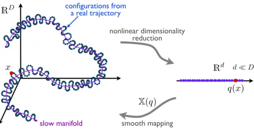
In reduced order modeling, we expect the system to abide by the reduced manifold, although the trajectories of the full system do not need to lie on it. This simplifying assumption introduces some error, compensated by a much faster simulation time. Figure4illustrates this idea, and the general pipeline of the current method. It is

slow manifold nonlinear dimensionality reduction d D smooth mapping configurations from a real trajectory

x

q

(

x

)

X

(

q

)

R

R

Figure 4: Sketch of the method to smoothly parametrize point-set manifolds. The set of high-dimensional snapshotsX(dark blue points) are embedded in low dimensions (light-blue points) by NLDR methods, possibly applied to the pruned snapshots for computational convenience. With the low-dimensional embedding at hand, the slow manifold hidden in the training setXis represented with a smooth, data-driven parametrizationX: A ⇢Rd _!RD_{. It is also possible to find the low-dimensional representationq(x)2} Rd _{of a new out-of-sample} configurationx2RD_{, whereq(x) is the pre-image byXof the closest-point projection ofxonM, found solving a nonlinear least-squares} problem [10].

clear that the low-dimensional space where the training set is embedded serves as a convenient parametric space. The embedded points inQare in general unstructured, and, although we show here examples ind=2, the method-ology is applicable to higher-dimensional embedded manifolds. Thus, a general method to compute on point-set manifolds demands a smooth approximation scheme for general unstructured nodes in multiple dimensions. The need for smoothness in the present application is shown in the Section below, e.g. Eq. (27). Here, we consider the localmax-entapproximants [12], a general meshfree method satisfying these requirements.

Letpa(q) denote the LME basis functions associated to the node setQ, defined in a subset of the convex hull

ofQ,A ⇢Rd_{. We parametrize the manifold as}

X:A !RD

q7 ! X

a

pa(q)xa, (12)

wherexa2RDare the full-sized snapshots, irrespective of the fact thatQmay have been found on the basis of the

pruned snapshots. 3.5. Reconstruction error

With a parametrization of the slow manifold at hand, it is possible to evaluate its quality by comparing high dimensional data with their reconstruction through the parametrization. Ideally, this is done with a test setZ =

{z1, . . . ,zM}⇢RD, di↵erent and possibly larger than the training set, samplingM. We can then define the relative

reconstruction error e= 1 M M X a=1 kza X(q(za))k kzak , (13)

wherek·kindicates the standardL2 norm computed as the Euclidian distance between two points inRD, whereas

q(x) maps high-dimensional points to low-dimensional representations, see Fig.4and [10]. For PCA, we have e= 1 M M X a=1 za PPT(za x)¯ x¯ kzak . (14)

4. Lagrangian mechanics in generalized coordinates

4.1. Constrained dynamics

Letx2RD_{denote the position in Cartesian coordinates of a mechanical system described by its Lagrangian}

as follows

L(x,x)˙ =T( ˙x) V(x)=1 2x˙

whereT is the kinetic energy, V the potential energy and M is the constant mass matrix. The corresponding Euler-Lagrange equations can be written as

Mx¨= @V

@x(x). (16)

We are interested in the constrained dynamics on a configuration manifoldM ⇢RD_{of dimensiond ⌧D. Let}

q2A ⇢Rd_{be the generalized coordinates given by NLDR as described above. We parametrizeMin terms of}

these generalized coordinates asx=X(q). By the chain rule, ˙x= DX(q) ˙q, and therefore we can formulate the constrained dynamics as L(q,q)˙ = 1 2q˙TM(q) ˙e q eV(q), (17) where e M(q)=DX(q)TM DX(q) and eV=V X. (18)

Since the mass matrix is in general configuration-dependent, this is an instance of non-separable Lagrangian. By Hamilton’s principle, the Euler-Lagrange equations of the reduced system, expressing the balance of linear momentum in curvilinear coordinates, are

d dt @L @q˙ @L @q =0. (19)

In the special case of PCA (or other linear methods), the manifold parametrization is affine,DX=P, and conse-quently the reduced mass matrix is not position dependent,Me=PTMP.

4.2. Discrete Lagrangian mechanics

We resort to variational principles to integrate in time the Euler–Lagrange equations; full details can be found in [21,22] and references therein. See also [23] for variational integrators for systems with configuration-dependent mass matrix. Starting with the action functional

S[q]=

Z t1

t0

L(q,q)˙ dt, (20)

for the system’s trajectoryq(t) inA satisfying the initial conditions, variational integrators are based on Hamil-ton’s principle, which states that the trajectories are stationary points of the action, S[q, q]=0 for all admissible

q.

In time-discrete Lagrangian mechanics (one step methods), the action integralS is replaced by an action sum Sd=

n 1 X j=0

Ld(qj,qj+1), (21)

whereLd : M⇥M ! R is the discrete Lagrangian, a function of two pointsq0 = q(t0), q1 = q(t1) 2 A

approximating the action in an interval as

Ld(q0,q1)⇡ Z t1

t0

L(q,q)˙ dt. (22)

The discrete Euler-Lagrange equations –the time-integration algorithm–, follow from making the action sum sta-tionary, e.g.@Sd/@qk=0, and are given by

D1Ld(qk,qk+1)+D2Ld(qk 1,qk)=0. (23)

The accuracy of the variational integrator is given by the order of the quadrature in Eq. (22). Specific numer-ical integration schemes can be obtained from this formalism. For concreteness, we derive here the discrete Euler-Lagrange equations for the generalized midpoint rule with configuration-dependent mass. Additionally, in

Appendix A, the resulting expressions for the trapezoidal rule for a configuration-dependent mass are given. For the generalized midpoint rule, the discrete Lagrangian approximating the action integral betweenq0 andq1 is

given by Ld(q0,q1)= t L ✓ (1 ↵)q0+↵q1,q1 _tq0 ◆ = t (₁ 2 ✓_q 1 q0 t ◆T e M⇣(1 ↵)q0+↵q1 ⌘ ✓q1 q0 t ◆ e V⇣(1 ↵)q0+↵q1 ⌘) , (24)

where↵2[0,1]. From Eqs. (23,24), we obtain the following equation forqk+1 0=@Sd @qk = t ( (1 ↵)D1L ✓ (1 ↵)qk+↵qk+1, qk+1 qk t ◆ ₁ tD2L ✓ (1 ↵)qk+↵qk+1, qk+1 qk t ◆) + t ( ↵D1L ✓ (1 ↵)qk 1+↵qk,qk qk 1 t ◆ + 1 tD2L ✓ (1 ↵)qk 1+↵qk,qk qk 1 t ◆) = t(1 ↵) (₁ 2 ✓_qk +1 qk t ◆T DMe⇣(1 ↵)qk+↵qk+1 ⌘ ✓qk+1 qk t ◆ DeV⇣(1 ↵)qk+↵qk+1 ⌘) (25) + t↵ (₁ 2 ✓_{qk qk 1} t ◆T DMe⇣(1 ↵)qk 1+↵qk ⌘ ✓qk qk 1 t ◆ DeV⇣(1 ↵)qk 1+↵qk ⌘) e M⇣(1 ↵)qk+↵qk+1 ⌘ ✓_{qk+1 qk} t ◆ +Me⇣(1 ↵)qk 1+↵qk ⌘ ✓_{qk qk 1} t ◆ .

These calculations require the directional derivative of the reduced mass matrix, and derivative of the reduced potential energy, computed as follows from the product and the chain rule

DM(q) ˙e q=YT(q,q)˙ M DX(q)+DX(q)TMY(q,q)˙ , (26) with

Y(q,q)˙ =D2X(q) ˙q, (27)

and

DeV(q)=DV(X(q))DX(q). (28)

It is also possible to obtain an expression for the generalized velocities associated to the Cartesian velocities at a point inMand tangent to it

˙

q=hDX(q)T DX(q)i 1DX(q)T x˙. (29)

It is clear from Eq. (27) that this formulation requires a smooth representation of the slow manifold. 4.3. Implementation and efficiency

From a practical viewpoint, the choice↵ =0 is most convenient in the time-stepping algorithm since then Eq. (25) is merely quadratic in qk+1. Otherwise, the resulting algorithm is implicit inqk+1 in a very nonlinear way, requiring third order derivatives ofX(q) for an iterative solution with Newton’s method. The implementation details for↵=0 in combination with Newton’s method are given inAppendix B.

It should be emphasized that the formulation presented above for the reduced dynamics involves evaluating the full model, which is computationally expensive for nonlinear systems such as that considered here. For instance, Eq. (28) involves computing the forces of the high-dimensional system. There has been an intense research activity on e↵ective reduction methods for nonlinear systems in recent years, which avoid altogether calculations involving the full model. These methods include piecewise linear approximations, or gappy reconstructions of the nonlinear terms, e.g. here DV(x), through interpolation [24] or least squares [15]. Such methods can be integrated with the proposed nonlinear representation of the low-dimensional configuration manifold, but are not implemented here. In fact, given the extreme low dimensionality of the reduced models (d  3 in the examples presented here), the full reduction of the system, without any reference toD, is very easily accomplished by interpolation of the reduced massM(q) and potentiale eV(q) on the parametric representation of the slow manifold, as discussed later.

5. Proof-of-concept example: a neo-Hookean oscillator

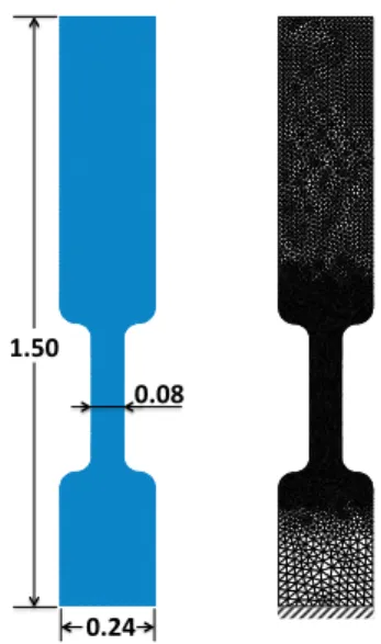
We show here the capabilities of the present method in a proof-of-concept problem, the dynamics of a hy-perelastic neo-Hookean body undergoing large deformations. We compare the proposed nonlinearly reduced dynamics against the standard reduced dynamics from a linear method (PCA). The geometry of the object and mesh are shown in Fig.5.

5.1. Training set

We simulated 35 trajectories for di↵erent initial conditions (position and velocity), with an explicit mid-point rule integration scheme. For each trajectory, a total number of 4·106_{time steps were computed and sampled with}

a frequency of 1/1000, resulting in 4000 snapshots per trajectory. In an o✏ine process, the first 500 snapshots were deleted to avoid poorly sampled regions arising from unlikely starting points. Further, due to the symmetry

0.24% 0.08% 1.50%

Figure 5: Sketch for the neo-Hookean hyperelastic solid in 2D (left) and the mesh used to compute the elastodynamics (right). The object is clamped at the bottom, and subject to gravity. The material parameters are =1000 andµ=500, and the model is discretized by 9428 linear

triangular elements and 4934 nodes.

of the problem, each retained snapshot was duplicated and mirrored. As the mesh is not structured, mirroring the snapshots requires interpolation.

As a result, a total of 245,000 full configurations in D =9,868 (4,934 nodes inR2_{) were obtained. These}

snapshots were then pruned by keeping only the nodes at the boundary, resulting in simplified snapshots in di-mensionDe=868, approximately one tenth ofD. In pruning the snapshots, one needs to balance compression and fidelity. For instance, we found that keeping only 100 points along the skeleton resulted in a poorer description of the dynamics. Finally, we decimated the pruned training set, down toNe=50,000 configurations inDe=868. For a schematic explanation we refer to Fig.1. From now on we will refer to the size and dimension of the resulting training set asNandD.

5.2. Intrinsic dimension

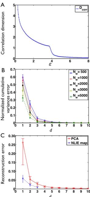
As discussed in Section3.5, we cana prioriestimate the intrinsic dimension underlying the data set. Figure

6illustrates how the correlation dimension (A) and the cumulative variance error of local PCA (B) provide hints, but not conclusive information for realistic training sets. These methods are blind to the origin of the data. The intrinsic dimension appears to be between 2 and 4, depending on the scale of observation. We evaluate the dimensiona posteriori(after dimensionality reduction on the parametrization of the slow manifold) by tracking the reconstruction error as a function of the dimension of the embedding, see Fig.6C. With PCA, it is straightforward to increase the dimension, while for the nonlinear methods, whose objective is to keepd as small as possible, we have only constructed one-, two- and three-dimensional slow manifolds. As expected for data with nonlinear correlations, it can be observed that the reconstruction error stemming from NLDR are significantly smaller than that given by PCA for a given dimension. The dimensionality estimations are consistent with thea priorimethods. From our experience, the most practical method of dimensionality estimation is tracking the cumulative variance error of local PCA. It is fast, easily made parallel, can be performed on pruned data, and does not need an embedding in low-dimension of the training set.

5.3. Dimensionality reduction

Figure7shows the two- and three-dimensional embeddings of the training set by PCA, Isomap and NLIE. It is obvious from the three-dimensional embeddings that the data has highly nonlinear correlations, i.e. the slow manifold is highly curved. As a result, it is not surprising that Isomap collapses some parts of the training set. In contrast, NLIE gently unrolls the curved manifold by introducing local distortions that minimize the global stress energy. A close visual inspection of the three-dimensional embedding provided by PCA or NLIE suggests that the data lies on a “thick” elongated hyper-surface.

The one-dimensional embedding of PCA can be found by projecting alongq1the two-dimensional embedding.

It is clear from the figure that this method will collapse far-away conformations, destroying the geometric struc-ture of the slow manifold. In contrast, the one-dimensional NLIE embedding provides a coarse, yet meaningful representation of the model.

0 2 4 6 8 0 1 2 3 4 5 D_corr Co rr el ati on di mens io n

A

B

C

Figure 6: (A) The correlation dimension method considers a closed ball of radius"at the center of each data point, and counts the number of points inside of this ball. The dimension is estimated by noting that the average number of countsC(") should grow linearly with"for 1D objects, quadratically for 2D entities, and so on, i.e.C(")/"d. The correlation dimension is then defined asdcorr(")=dlogC(")/dlog". It is a scale-dependent quantity that should be interpreted carefully: at very large",dcorr⇡0 as the data set looks like a single point, while for small", the dimension is overestimated by the presence of noise. (B) Mean of the normalized cumulative variance error from local PCA (±25th and 75th percentiles), 1 ⇣Pd

i=1 i/PiD=1 i⌘, computed in small local subsets of the data whereNwis the window size. idenote the eigenvalues of the local covariance matrix arranged in decreasing order. The intrinsic dimensiondfor each of these patches is selected such that it preserves a given fraction of the variance of the original data. In contrast with the global correlation dimension, this method provides a local estimation of the intrinsic dimension. (C) Mean of the reconstruction error as defined in Eqs. (13,14) (±25th and 75th percentiles). The reconstruction error is a measure of the dissimilarity between the original high-dimensional data points and their reconstruction through the slow manifold parametrization, hereM=50,000.

We finally note that, in principle, it is possible to define a nonlinear parametrization of the slow manifold such as that in Eq. (12) on the basis of PCA embeddings. However, from our experience in this and other applications, these low-dimensional embeddings introduce larger distortions (see Fig. 3B) and are not robust for significantly curved training sets.

5.4. Parametrization of the slow manifold

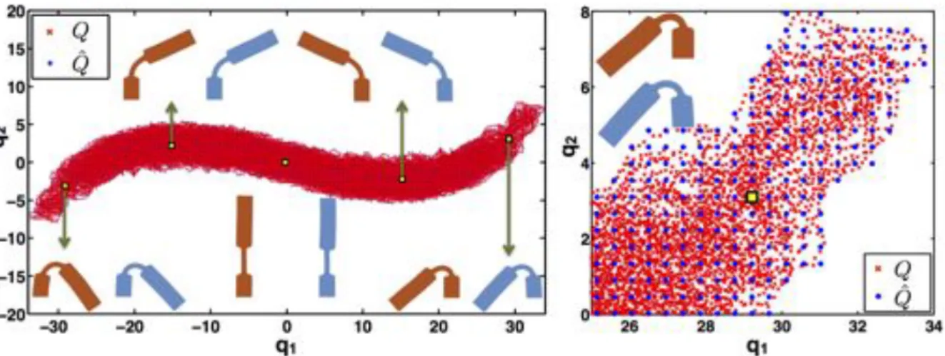
We follow Eq. (12) to parametrize smoothly the slow manifold from the embedding in low-dimension,X(q), with LME basis functions. Details about the calculation of these meshfree approximants and their spatial deriva-tives can be found in [12,25]. The noise filtering can be controlled with the width of the LME basis functions. Figure8shows in more detail the two-dimensional embedding found with NLIE, where the red points represent

Figure 7: Two-(left) and three-dimensional (right) embeddings obtained with PCA (top), Isomap (center) and NLIE (bottom). The colormap, indicating the Euclidean distance to the first configuration of the training set, is only provided as visual guide.

Figure 8: Two-dimensional embeddingQobtained from the original training setXwith NLIE (red points), and subsampled node set ˆQ(blue points), over the entire low-dimensional embedding (left). For some selected ˆqb, we depict the corresponding configuration ˆxq obtained from the least squares fit, and the closest conformation from the original training set. A magnification of the upper-right corner of the two-dimensional embedding (right).

the setQ. An obvious drawback of defining_X(q) =PN_a=1pa(q)xais thatNcan be very large, here 50,000, and

therefore the evaluation of this mapping, required at each time-step, can be quite expensive. In fact, this mapping parametrizes a relatively simple slow manifold, and the large number of samples is only required to provide a statistically representative low-dimensional embedding. For computational convenience, we subsample the de-scription of the slow manifold as follows. We divide the low-dimensional embedding space in equally spaced bins of sizehbin = L/nbin, whereLis the length of the low-dimensional embedding alongq1 andnbinthe number of

bins in this direction.hbinshould be commensurate to the geometrical features of the slow manifold. This defines

a regular grid, from which we retain the points lying in well-sampled regions of the low-dimensional embedding, the blue points in Fig.8, that we denote by ˆQ = {qˆ1,qˆ2, . . . ,qˆNˆ}with ˆN ⌧ N. We then define the LME basis

a least-squares criterion (see also [10]) min {xˆ1,...xˆNˆ} N X a=1 xa ˆ N X b=1 ˆ pb(qa) ˆxb 2 . (30)

In the example shown in Fig.8, we selectednbin = 150, leading to a subsampling of the slow manifold from

N =50,000 to ˆN =2,115 control points. The optimal value ofnbin is problem-dependent, and is influenced by

the sampling of the configurational space and the features of manifold.

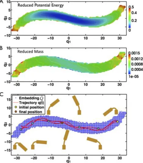
Figure 9: (A) Reduced potential energyeV(q). (B) Total reduced massP_i,jMei j(q). (C) Reduced trajectory in the two-dimensional embedding from NLIE, over seven large amplitude oscillations of the system. The initial, final, and selected snapshot positions are highlighted.

We can time-integrate the reduced dynamics with the methods outlined in Section4.2and redefine the smooth mapping asX(q)=PN_bˆ₌₁pˆb(q) ˆxb, leading to a numerical trajectory in the low-dimensional spaceq(t). The

non-linearly reduced dynamics are fully determined by the e↵ective potential energyeV(q) and the reduced massM(q).e Figure9A shows the e↵ective potential, whereas Fig.9B shows the total reduced mass in the two-dimensional embedding. It can be observed that the reduced mass, which is in fact the square mass-weightedL2norm of the

derivative of the slow manifold parametrization, see Eq. (18), is nearly constant except at the boundaries of the region of interest. At the boundary, it is not surprising that the quality of the mappingX(q) is degraded. Yet, these regions are visited seldom due to their high potential energy.

Figure9C shows an example of reduced dynamicsq(t). Visually, these dynamics retain the qualitative features of the full, high-dimensional dynamics, with high amplitude oscillations. In the examples below, we consider both PCA- and NLIE-reduced dynamics. We always use a midpoint rule with↵=0, with a time step t=10 4in the reduced simulations (5 times larger than that of the full dynamics). For PCA, details about the time-integration are given inAppendix A, whereas for NLIE, due to the mass position-dependency, the algorithm is nonlinear and quasi-explicit (only the gradient ofV(x) is required). We use Newton’s method, seeAppendix B.

For a more quantitative assessment of the quality of the reduced dynamics, we compare them to the full dynamics,x(t), with the following metric

Z t1 t0 D x(t),_X(q(t)) dt= Z t1 t0 Z ⌦0 'h(x(t)) 'h(X(q(t))) 2dV !1/2 dt, (31)

where here'h(x) denotes the finite element deformation mapping defined from the nodal positions x. In

prac-tice, we sample the time-integral at the time-stepstj = j t, and compute a non-dimensional distance between

trajectoriesDas D= Pn j=0 p (xj X(qj))TM(xj X(qj)) Pn j=0 q xT jM xj , (32)

whereMis the mass matrix of the elastic body computed at the reference configuration.

Real%dynamics% Nonlinear%reduced%dynamics%d=3% Linear%reduced%dynamics%d=10% Linear%reduced%dynamics%d=20% t=%0.0% t=27.5% t=36.0% t=%7.5% t=%15.0% t=23.0% t=43.5% t=50.0% 00 10 20 30 40 50 0.05 0.10 0.15 0.20 0.25 0.30 time d= 7 PCA d=10 PCA d=13 PCA d=20 PCA d= 1 n_bin100 d= 2 n_bin125 d= 3 n_bin 60

Figure 10: Snapshots during the time evolution of a high-dimensional trajectoryx(t), and the reduced trajectoriesX(q(t)) obtained from PCA and NLIE (left). The quality of the reduced dynamics is measured by the relative cumulative distance betweenx(t) andX(q(t)) (right).

Figure10compares, both visually with conformations at selected instants, and quantitatively withD, the full dynamics with the reduced dynamics obtained either by PCA with various dimensions, or by NLIE with dimen-sions one, two, and three. The results indicate that more than 10 PCA modes are needed to capture the dynamics of the system. With only one nonlinear generalized coordinate, we obtain a poor description of the system, com-parable to those observed with between 7 and 10 PCA modes. This is not surprising, since the large amplitude oscillations lead to a highly nonlinear configuration manifold, and therefore PCA needs to properly describe its affine hull for reasonable results. As the numbed of PCA modes increases, we obtain accurate dynamics. Strik-ingly, with only two or three nonlinear dimensions, we obtain results that lie between those given by 10 and 20 PCA modes. The results suggest that in this example, the affine hull of the slow manifold has tens of dimensions, highlighting the benefit of nonlinear reduced descriptions.

It is interesting that, while correct PCA-reduced dynamics require more than 10 modes, Fig.6C suggests that, on the basis of the reconstruction error, the slow manifold can be accurately captured by less than 10 modes. This discrepancy highlights the limitations of statistical/geometric quantifications of the dimensionality, which ignore the physics altogether. The section below provides more insight on a related topic.

5.5. Energy leak of the slow modes

Figure 11shows the reduced trajectory in the three-dimensional embedding from NLIE, whereas Fig. 12

shows the energy evolution of the full (left) and the reduced (right) dynamics for d=3 (nbin =60) over eighteen

oscillations. It can be observed that, when the system visits its symmetric configuration, the potential energy lies close to its minimum while the kinetic energy is highest. Around this point, high frequency oscillations in the energy can be observed, suggesting a transfer to high frequency modes, which is consistent with the visualization of the dynamics. The reduced dynamics exhibit similar features, but with only two transversal dimensions to the main nonlinear coordinate, the features are significantly blunter. This observation raises the question of the long-time energy behavior of the reduced dynamics.

To investigate numerically this issue, we consider a very long trajectory of the full system, project the dynamics onto the PCA modes, and then compute the energy of the projected trajectory. Note that we do not perform here

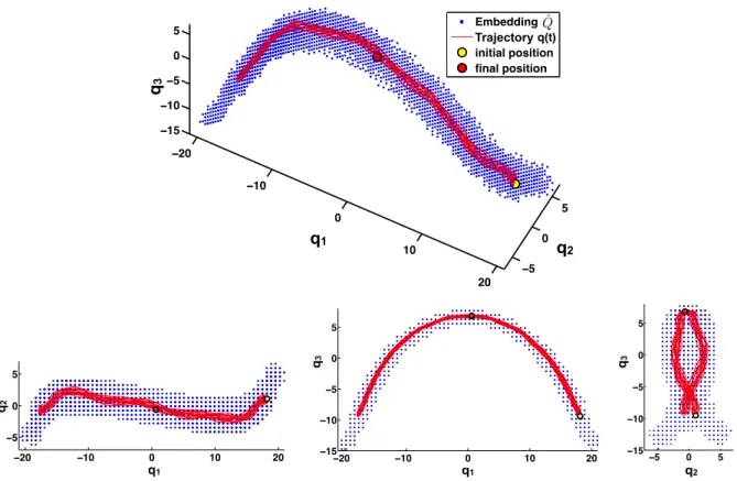
−20 −10 0 10 20 −5 0 5 −15 −10 −5 0 5 Embedding Q_{Trakectory q(t)} initial position final position ˆ Q q1 _q 2 q3 −5 0 5 −15 −10 −5 0 5 −20 −10 0 10 20 −5 0 5 −20 −10 0 10 20 −15 −10 −5 0 5 q1 q1 q2 q2 q 3 q3 Trajectory

Figure 11: Reduced trajectory in the three-dimensional embedding obtained with NLIE, over eighteen large amplitude oscillations of the system. The initial and final embedded positions are highlighted.

0 5 10 15 20 25 30 35 40 45 50 −0.2 −0.1 0 0.1 0.2 0.3 0.4 0.5 time E_TOT E KIN E_POTint E POT ext 0 5 10 15 20 25 30 35 40 45 50 −0.2 −0.1 0 0.1 0.2 0.3 0.4 0.5 time E TOT E_KIN E POT int E_POText

Figure 12: Energy evolution for the full system trajectory (left), and for the reduced trajectory with a three-dimensional nonlinear embedding (right).

any PCA-reduced trajectory, but rather analyze a full trajectory from the viewpoint of the PCA-reduced model. We also recall that the system is conservative, and therefore the total energy should remain constant.

Figure13shows the time-evolution ofE(t) andE(t) fore d=20,50,100,200,500,1000,2000 PCA modes over

a very long simulation. Interestingly, there is a significant and monotonic flow of energy from the low modes into the high-frequency modes. Increasing the reduced dimension, e↵ective at short times, only slightly reduces the energy leak at long times. Once this energy is “thermalized” in the high-frequencies, it does seem to return to the low-frequency modes. Thus, the system described by the reduced coordinates is no longer conservative. These results suggest the need for modeling the net e↵ect of the disregarded degrees of freedom on the reduced dynamics, as is done in the large eddy simulation of turbulence. The long experience in coarse-graining of molecular systems and non-equilibrium statistical mechanics [26], or optimal prediction [27] could be useful in this regard.

10−3 10−2 10−1 100 101 102 0.22 0.23 0.24 0.25 0.26 0.27

time

E(t)

Figure 13: Total energy evolution of the full system and total energy projected onto the reduced models by PCA for di↵erent numbers of

eigenvectors,d=20,50,100,200,500,1000,2000. 6. Concluding remarks

We have proposed a novel method for reduced order modeling and exercised it on large-deformation nonlinear elastodynamics. In contrast with most approaches, the reduced model is not an affine one, as given e.g. by PCA or POD. Instead, we use modern NLDR methods to embed an ensemble of snapshots in low-dimensions, and then build from this low-dimensional embedding a smooth representation of the system in terms of nonlinear, data-driven, generalized coordinates. The underlying hypothesis is that many systems evolve on a nonlinear, low-dimensional slow manifold, and that by acknowledging the nonlinearity, it is possible to build more efficient and insightful reduced models. We discuss in detail the practical aspects of the methodology, which requires extra data structures and procedures, but results in a much more compact description, which presumably leads to more insight. For instance, the reduced dynamics of the finite element equations of elastodynamics have a position-dependent mass, and we derive the corresponding variational time-integrators.

We have tested the method in a proof-of-concept example, a structure made out of a Neo-Hookean material undergoing large amplitude oscillations. By comparing the nonlinearly reduced dynamics with those generated by a linear methods, here PCA, our results suggest that nonlinearity reduces the number of dimensions required for an accurate description: two or three nonlinear generalized coordinates are equivalent to between 10 and 20 PCA modes. Below 10 PCA modes, the linear reduced model cannot capture even qualitatively the dynamics. Note that the PCA model is linear with regards to the structure of the reduced manifold, but fully nonlinear in that the underlying model is nonlinear elasticity. Our analysis of the intrinsic dimension of the ensemble of snapshots suggests that the dynamics lie on a slow manifold of dimension between 2 and 4. PCA only works if it adequately describes the affine hull of the slow manifold, which is of significantly higher dimension. In contrast, two or three nonlinear coordinates capture the essential features of the system. We have also shown that the nonlinearly reduced description can be coarsened in many ways to speed-up the evaluation of the slow manifold. Having a fast and optimally reduced description of the system is very attractive in some applications such as optimal control.

One of the limitations of the nonlinear reduction method is that increasing the dimension requires significantly larger training sets, so that the low-dimensional embedding of the snapshots is not too sparse. Otherwise, the parametrization of the slow manifold becomes problematic. In our proof-of-concept example, we attempted to reachd=4, but found that the mappingX(q) was of poor quality (very large derivatives) close to the boundary of the region of interest, leading to instabilities in the time-integration. This issue can be resolved hierarchically. For instance, the two-dimensional embedding can be used to generate new training trajectories from poorly-sampled regions on the boundary, thereby improving the sampling of the slow manifold. According to our preliminary calculations, a subsequent dimensionality reduction process leads to better low-dimensional embeddings, also in higher dimensions. Our experience also suggests that, beyond mere geometric similarity, which cannot distin-guish high-frequency but possibly highly energetic features, the dimensionality reduction could take into account information about the mechanics of the snapshots, such as their potential energy as an extra coordinate inxa. We

Finally, we have shown that our Hamiltonian system of interest, when described in terms of a reduced model, is no longer conservative. We find that the energy leak is significant for long times, and cannot be e↵ectively controlled by increasing the PCA dimension to 1000’s. This suggests that reduced order simulation should be accompanied by modeling the net e↵ect of the disregarded degrees of freedom on the reduced system.

Acknowledgments

We acknowledge the support of the European Research Council under the European Community’s 7th Framework Programme (FP7/2007-2013)/ERC grant agreement nr 240487. MA acknowledges the support received through the prize “ICREA Academia” for excellence in research, funded by the Generalitat de Catalunya.

Appendix A. Variational integrator schemes

Appendix A.1. Midpoint rule with constant mass

We have seen that for PCA model reduction, the mass matrix is not position-dependent. The discrete La-grangian for the generalized midpoint rule is then

Ld(q0,q1)= t L ✓ (1 ↵)q0+↵q1,q1 _tq0 ◆ = t (₁ 2 ✓_{q1 q0} t ◆T e M✓q1 q0 t ◆ e V⇣(1 ↵)q0+↵q1 ⌘) , (A.1)

where↵₂[0,1]. By making the discrete action stationary,@Sd

@qk =0, we find as discrete Euler–Lagrange equations

0=@Sd @qk = e M✓qk qk 1 t ◆ e M✓qk+1 qk t ◆ t(1 ↵)DVe⇣(1 ↵)qk+↵qk+1 ⌘ t↵DVe⇣(1 ↵)qk 1+↵qk ⌘ , (A.2) which for↵=0 gives the classical second-order Newmark explicit integration scheme

e

M qk+1 2qk+qk 1

t2 !

= DeV(qk). (A.3)

For PCA, the resultingd⇥dlinear system of equations is

PT_MP qk+1 2qk+qk 1

t2 !

= PTDV(Pqk+x)¯. (A.4)

Appendix A.2. Midpoint rule with configuration-dependent mass and↵=0

We consider a midpoint rule with↵=0 to integrate the action betweenq₀andq₁, which in the case of a mass configuration-dependent system generates the following discrete Lagrangian

Ld(q0,q1)= t L ✓ q0,q1 _tq0 ◆ = t ( 1 2 ✓_{q1 q0} t ◆T e M(q0) ✓_{q1 q0} t ◆ e V(q0) ) . (A.5)

The discrete Euler-Lagrange equations are then 0= @Sd @qk = t (₁ 2 ✓_q k+1 qk t ◆T DM(qe k) ✓_q k+1 qk t ◆ DeV(qk) ) e M(qk) ✓_qk +1 qk t ◆ +M(qe k 1) ✓_{qk qk 1} t ◆ . (A.6)

Appendix A.2.1. Generalized trapezoidal rule with configuration-dependent mass

The discrete Lagrangian for the generalized trapezoidal rule with configuration-dependent mass is

Ld(q0,q1)= t ⇢ (1 ↵)L ✓ q0,q1 _tq0 ◆ +↵L ✓ q1,q1 _tq0 ◆ = t ( 1 2 ✓_q 1 q0 t ◆T_⇣ (1 ↵)Me(q0)+↵Me(q1) ⌘ ✓q1 q0 t ◆ ⇣ (1 ↵)Ve(q0)+↵Ve(q1) ⌘) . (A.7)

The discrete Euler-Lagrange equations are then 0= @Sd @qk = t(1 ↵) ( D1L ✓ qk,qk+1_t qk ◆ +D₂L ✓ qk,qk+1 _t qk ◆ ₁ t !) + t ( D2L ✓ qk+1,qk+1_t qk ◆ ✓ _↵ t ◆ +D₂L ✓ qk 1,qk q_tk 1 ◆_{(1 ↵)} t ) + t↵ ( D1L ✓ qk,qk qk 1 t ◆ +D₂L ✓ qk,qk qk 1 t ◆ ₁ t ) = t(1 ↵) (₁ 2 ✓_{qk+1 qk} t ◆T DM(qe k) ✓_{qk+1 qk} t ◆ DeV(qk) ) ⇣ (1 ↵)M(qe k)+↵M(qe k+1) ⌘ ✓qk+1 qk t ◆ +⇣(1 ↵)M(qe k)+↵M(qe k 1)⌘ ✓qk q_tk 1 ◆ + t↵ (₁ 2 ✓_{qk qk 1} t ◆T DM(qe k) ✓_{qk qk 1} t ◆ DeV(qk) ) . (A.8)

Appendix B. Newton’s method for the midpoint rule and↵=0

We first define the residual of the discrete Euler–Lagrange equations as r(qk+1)=

@Sd

@qk, (B.1)

where@S/@qkis given by the Eq. (25). The first derivative of the residual is

J(qk+1)= @r(qk+1) @qk+1 = ✓_qk +1 qk t ◆T DM(qe k) 1 tM(qe k). (B.2)

The derivative of the reduced mass matrix involves second order derivatives of the parametrization X(q), see e.g. our work in thin shell analysis [10]. We numerically solve the discrete Euler-Lagrange equations in each time step by iterating qi+1 k+1 =q i k+1 J 1(q i k+1)r(q i k+1). (B.3)

As an initial seed for Newton’s method, we take thatDM(qe k)=0, and thenq0_k+1can be computed by solving the

d⇥dsystem e M(qk) t 0 BBBB@q0k+1 qk t 1 CCCCA= M(qe k 1) t ✓_{qk qk 1} t ◆ DeV(qk). (B.4)

Appendix C. Nonlinear Locally Isometric Embedding

In this appendix, we describe an iterative procedure that finds a low-dimensional embedding as isometric as possible to the high-dimensional input. This is performed by minimization of a cost or stress functionES, which

measures the di↵erence between the distances computed in low- and high-dimensions. This method is based on the work by [28], but di↵ers in the way we measure distances in the ambient space, and in the stress energy. Here, we consider geodesic instead of Euclidean distances. The geodesic distance on the manifold is approximated as the shortest path distance in a graph made withkG nearest neighbors (where subindexGrefers to the graph

distance⇡geodesic distance), in the same way that in the Isomap method [17] but di↵ering in that Isomap needs to compute a full distance matrix.

We define the stress energy, to be minimized by the set of embedded configurationsQ={q₁, . . . ,qN}2Rd, as ES(Q)=↵E1(Q)+(1 ↵)E2(Q), (C.1) where E1(Q)= 1 2 N X i=1 X j2N(i) |qi j| |xi j| 1 !2 , (C.2) and E2(Q)= 1₂ N X i=1 X j2N(i) |xi j| |qi j| 1 !2 , (C.3)

where↵2(0,1],qi j =qi qj,xi j=xi xj, andN(i) contains the indices for the firstkG nearest neighbors ofxi.

The second term,E2, prevents nearby points from colliding. From our experience,↵should be close to 1. If the

input data is very noisy in the normal direction to the manifold, a small↵could lead to a very slow convergence,

or even divergence. In such cases, we recommend 0.9999  ↵  1. In our experiments we commonly use

↵=0.99 0.999 ford >1, and↵=1 ford=1.

In our definition of stress function, we take into account only a moderate number of neighboring points, which give an accurate idea of the local geometry of the manifold. Commonly, in our experiments we usekG= 200 1000. Note that in the Isomap method,kG=N. In the original work of Sammon [28], all the pairs distances are needed, which implies storing and manipulating a full matrix, whereas here we handle a sparse matrix. Similar methods have been proposed, for instance see the works [29,30].

We numerically solve the nonlinear optimization problem of minimizingES by first iterating with a

limited-memory Broyden-Fletcher-Goldfarb-Shanno (L-BFGS) algorithm [31] with a coarse tolerance, and then moving to Newton’s method with a Brent’s line search with a tighter tolerance. The gradient of the stress energy is

@ES @qi =↵ @E1 @qi +(1 ↵) @E2 @qi, (C.4) where @E1 @qi = X j2N(i) |qi j| |xi j| |xi j|2 ! _q i j |qi j|+ X j2Ne(i) |qi j| |xi j| |xi j|2 ! _q i j |qi j|, (C.5) @E2 @qi = X j2N(i) |qi j| |xi j| |qi j|2 ! _q i j |qi j| |xi j| |qi j|+ X j2Ne(i) |qi j| |xi j| |qi j|2 ! _q i j |qi j| |xi j| |qi j|. (C.6)

The dual index list_Ne(i) toN(i) is built in such a way that_Ne(i) returns the indices jcontainingiin theirs index listsN(j). Finally, the Hessian ofES(q) is

@2ES @qi@qj =↵ @2E1 @qi@qj+(1 ↵) @2E2 @qi@qj. (C.7)

The first term contributes diagonal terms

@2E1 @q2_i = X j2N(i) " _q i j |qi j|⌦ qi j |qi j| ! |xi j| |qi j|+ |qi j| |xi j| |qi j| ! I # 1 |xi j|2 + X j2_Ne(i) " _q i j |qi j|⌦ qi j |qi j| !_|x i j| |qi j| + |qi j| |xi j| |qi j| ! I # 1 |xi j|2, (C.8)

and o↵-diagonal terms when jis inN(i) orNe(i), given by

@2E1 @qi@qj = " _q i j |qi j|⌦ qi j |qi j| !_|x i j| |qi j|+ |qi j| |xi j| |qi j| ! I # ₁ |xi j|2. (C.9)

From the second term of the stress energy, we have

@2E2 @q2_i = X j2N(i) " _q i j |qi j|⌦ qi j |qi j| ! |xi j| |qi j|+ |qi j| |xi j| |qi j| ! I ₃qi j |qi j|⌦ qi j |qi j| !# |xi j| |qi j|3 + X j2_Ne(i) " _q i j |qi j|⌦ qi j |qi j| !_|x i j| |qi j|+ |qi j| |xi j| |qi j| ! I ₃qi j |qi j|⌦ qi j |qi j| !# _|x i j| |qi j|3, (C.10)

and @2E2 @qi@qj = " _q i j |qi j|⌦ qi j |qi j| !_|x i j| |qi j|+ |qi j| |xi j| |qi j| ! I ₃qi j |qi j|⌦ qi j |qi j| !# _|x i j| |qi j|3. (C.11) References

[1] P. Krysl, S. Lall, J. E. Marsden, Dimensional model reduction in non-linear finite element dynamics of solids and structures, International Journal for Numerical Methods in Engineering 51 (4) (2001) 479–504.

[2] S. Niroomandi, I. Alfaro, E. Cueto, F. Chinesta, Real-time deformable models of non-linear tissues by model reduction techniques, Computer Methods and Programs in Biomedicine 91 (2008) 223–231.

[3] M. Meyer, H. G. Matthies, Efficient model reduction in non-linear dynamics using the karhunen-lo`eve expansion and

dual-weighted-residual methods, Computational Mechanics 31 (2003) 179–191.

[4] P. Kerfriden, O. Goury, T. Rabczuk, S. Bordas, A partitioned model order reduction approach to rationalise computational expenses in nonlinear fracture mechanics, Computer Methods in Applied Mechanics and Engineering 256 (2013) 169 – 188.

[5] J. Lee, M. Verleysen, Nonlinear Dimensionality Reduction, Information science and statistics, Springer, New York, NY, USA, 2007. [6] A. J. G´amez, C. S. Zhou, A. Timmermann, J. Kurths, Nonlinear dimensionality reduction in climate data, Nonlinear Processes in

Geophysics 11 (2004) 393–398.

[7] P. Das, M. Moll, H. Stamati, L. Kavraki, C. Clementi, Low-dimensional, free-energy landscapes of protein-folding reactions by nonlinear dimensionality reduction, Proceedings of the National Academy of Sciences 103 (26) (2006) 9885–9890.

[8] W. M. Brown, S. Martin, S. N. Pollock, E. A. Coutsias, J.-P. Watson, Algorithmic dimensionality reduction for molecular structure analysis, The Journal of Chemical Physics 129 (6) (2008) 064118.

[9] J. Vanderplas, A. Connolly, Reducing the dimensionality of data: Locally linear embedding of sloan galaxy spectra, The Astronomical Journal 138 (5) (2009) 1365–1379.

[10] D. Mill´an, A. Rosolen, M. Arroyo, Nonlinear manifold learning for meshfree finite deformations thin shell analysis, International Journal for Numerical Methods in Engineering 93 (7) (2013) 685–713.

[11] M. Arroyo, L. Heltai, D. Mill´an, A. DeSimone, Reverse engineering the euglenoid movement, Proceedings of the National Academy of Sciences of USA 109 (2012) 17874.

[12] M. Arroyo, M. Ortiz, Local maximum-entropy approximation schemes: a seamless bridge between finite elements and meshfree methods, International Journal for Numerical Methods in Engineering 65 (13) (2006) 2167–2202.

[13] F. Chinesta, A. Ammar, E. Cueto, Recent advances and new challenges in the use of the proper generalized decomposition for solving multidimensional models, Archives for Numerical Methods in Engineering 17 (2010) 327–350.

[14] D. Amsallem, C. Farhat, An online method for interpolating linear parametric reduced-order models, SIAM Journal of Scientific Com-puting 33 (2011) 2169–2198.

[15] R. M. Everson, L. Sirovich, The karhunen–lo`eve transform for incomplete data, J. Opt. Soc. Am. A 12 (1995) 1657–1664. [16] S. Bouix, K. Siddiqi, A. Tannenbaum, Flux driven automatic centerline extraction, Medical Image Analysis 9 (3) (2005) 209–221. [17] J. Tenenbaum, V. de Silva, J. Langford, A global geometric framework for nonlinear dimensionality reduction, Science 290 (2000)

2319–2323.

[18] S. T. Roweis, L. K. Saul, Nonlinear dimensionality reduction by locally linear embedding, Science 290 (2000) 2323–2326. [19] K. Pearson, On lines and planes of closest fit to systems of points in space, Philosophical Magazine 2 (6) (1901) 559–572. [20] M. P. do Carmo, Di↵erential geometry of curves and surfaces, Prentice-Hall, 1976.

[21] J. Marsden, M. West, Discrete mechanics and variational integrators, Acta Numerica 10 (2001) 357–514.

[22] A. Lew, J. E. Marsden, M. Ortiz, M. West, Variational time integrators, International Journal for Numerical Methods in Engineering 60 (1) (2004) 153–212.

[23] P. Mata, A. J. Lew, Variational time integrators for finite dimensional thermo-elasto-dynamics without heat conduction, International Journal for Numerical Methods in Engineering 88 (2011) 1–30.

[24] S. Chaturantabut, D. C. Sorensen, Nonlinear model reduction via discrete empirical interpolation, SIAM Journal of Scientific Computing 32 (2010) 2737–2764.

[25] A. Rosolen, D. Mill´an, M. Arroyo, On the optimum support size in meshfree methods: a variational adaptivity approach with maximum entropy approximants, International Journal for Numerical Methods in Engineering 82 (7) (2010) 868–895.

[26] P. Espa˜nol, Statistical Mechanics of Coarse-Graining, Lecture Notes in Physics, Springer-Verlag, 2003.

[27] A. Chorin, A. Kast, R. Kupferman, Optimal prediction of underresolved dynamics, Proceedings of the National Academy of Sciences 95 (1998) 4094–4098.

[28] J. W. Sammon, A nonlinear mapping for data structure analysis, IEEE Transactions on Computers 18 (1969) 401–409.

[29] J. H´erault, A. Oliva, A. Gu´erin-Dugu´e, Scene categorisation by curvilinear component analysis of low frequency spectra, in: M. Verleysen (Ed.), Proceedings of the 5th European Symposium on Artificial Neural Networks, Bruges, Belgium, 1997, pp. 91–96.

[30] J. Lee, A. Lendasseb, M. Verleysen, Nonlinear projection with curvilinear distances: Isomap versus curvilinear distance analysis, Neu-rocomputing 57 (2004) 49–76.