Beyond the shared frailty model

(1)

Available at:

http://hdl.handle.net/2078.1/150625

[Downloaded 2019/04/19 at 11:11:35 ]

Munda, Marco

Abstract

This thesis deals with frailty modelling, a framework devised to analyse clustered survival data. The main focus is on modelling the frailty term. The frailty term captures the dependence of survival times within a cluster and the heterogeneity between clusters. Typical is that the frailty term is treated as a random effect. Different distributions have been proposed to model the frailty term. Contributions of this thesis include a unified framework for fitting the frailty model with different frailty distributions, a new diagnostic plot to evaluate the frailty distribution assumption, a simulation study to assess robustness of regression inference against frailty misspecification, and a method to test for decreasing cluster heterogeneity in a new time-varying frailty model. Also presented is a first step towards modelling spatial dependence in survival data by means of spatially correlated frailties.

Document type : Thèse (Dissertation)

Référence bibliographique

(2)

Beyond the shared frailty model

Goodness-of-fit, decreasing heterogeneity and spatial de-pendence

A thesis submitted in partial fulfillment of the requirements for the degree of Docteur en Sciences, Université catholique de Louvain, September 2014

Marco Munda

Thesis committee:

Catherine Legrand, supervisor (Université catholique de Louvain) Ingrid Van Keilegom, President (Université catholique de Louvain) Philippe Lambert (University of Liège, Université catholique de Louvain) Paul Janssen (Hasselt University)

Luc Duchateau (Ghent University)

Hein Putter (Leiden University Medical Center) Virginie Rondeau (Université Bordeaux Segalen)

(3)

(4)

“

Statisticians, like artists, have the bad habit of

falling in love with their models.

(5)

(6)

Acknowledgements

This thesis was conducted at the Institute of Statistics, Biostatistics and Actuarial Sciences (ISBA) at the Université catholique de Louvain, which I am leaving after four years. I would like to take this opportunity to thank a number of people.

I thank my supervisor, Catherine Legrand. Catherine, thank you for the trust you placed in me, for the freedom you gave me, and for making this a pleasant experience.

From the start I benefited greatly from discussions and collaborations with Paul Janssen and Luc Duchateau. Paul, thank you for your advice and all the guidance you provided along the way. On many occasions we discussed time-varying frailties, but the support you showed me has always been constant. Luc, thank you for your enthusiasm and your continuous encouragement. You always had a kind word for me! Thank you also for entrusting me with the “malaria project”.

I thank the jury members for their interest and their suggestions during my private defence. Ingrid, Hein, I will remember that you always greeted me with a smile. Virginie, thank you for inviting me to join the Institute of Public Health, Epidemiology and Development at the University of Bordeaux and for the warm welcome during my visit.

My thanks are extended to the administrative staff of ISBA, with a special thank you to Nancy Guillaume. Nancy, thank you for helping me whenever I needed. I also thank the SMCS, the statistical consulting service of ISBA, which gave me the opportunity to get my hands dirty with real data.

Finally, I thank Anne, the best colleague ever! I also thank Adrien, Alain, Alexandra, Alina, Anna, Aurélie, Benjamin, Catherine, Cédric, Céline, Eduardo, Federico, Habiba, Jennifer, Maïlis, Mathieu, Michał, Nathalie, Nathan, Nicolas, Sylvie, Vincent, and Yassin with whom I loved spending the past four years.

(7)

(8)

1 Introduction

1.1 Outline

In survival analysis, the outcome of interest (response variable) is a time-to-event endpoint, also called survival endpoint, e.g. time to death in cancer clinical trials. The central problem in the analysis of time-to-event endpoints is the presence of censoring. In its most common form (right censoring), censoring occurs when the follow-up is interrupted prior to the event’s occurrence. In that case, only a lower boundary is known for the event time. Section 1.2 provides a general, practical overview of survival analysis. Topics covered include terminology, special features of survival data, working assumptions, and standard methods of analysis to deal with censored data (non-parametric Kaplan-Meier survival curve, parametric Weibull regression, semi-parametric Cox re-gression). Further details can be found in textbooks, e.g. Collett (2003). Standard methods in survival analysis require independent event times, given the covariate information. In practice, many studies in-volve clusters. Examples of clusters include families, geographical areas, centres participating in a clinical trial, etc. Within a cluster, data are typically dependent. This thesis focuses on the frailty model, introduced in Section 1.3, to account for the dependence in clustered survival data. In the frailty model framework, the within-cluster association is taken into account by means of a cluster-specific factor, the frailty term. Typ-ical for this model is that the frailty term is treated as a random effect. Random effects for survival data were first considered in Beard (1959) and Vaupel et al. (1979) to improve the fit of mortality models at ad-vanced ages. In these early papers, the frailty term acts at the individ-ual level as an unobservable factor in the mortality model and indicates that “frail” people have an increased risk of death. The distribution of the individual-specific frailty term provides a way to model

(13)

served/unexplained variation in susceptibility to death (heterogeneity) in the population.

Applications of the frailty model to clustered data were first dis-cussed in Clayton (1978) for studies of familial aggregation of disease. Due to, for example, genetic and environmental factors, susceptibility to disease varies from family to family. Hence, variability in outcome among relatives tends to be lower than variability in outcome between non-relatives. In statistical terms, this translates into (i) unobserved heterogeneity between families, and into (ii) association among observa-tions from the same family. Frailty models with a cluster-specific frailty term, also called shared frailty models, have been developed over the last three decades to deal with this type of data.

For an introduction to the most important aspects of the frailty model methodology, as well as an extensive list of references to major papers and recent developments in the area, see Duchateau & Janssen (2008) and Wienke (2010). Nice applications illustrating the usefulness of the frailty model in practice include Michiels et al. (2005), Legrand et al. (2006), and Rondeau et al. (2010).

This thesis is organised around three research themes of current inter-est in frailty modelling. The content of each research theme is outlined below.

Part I – The frailty distribution

Different distributions have been proposed to model the frailty term. To mimic the normal random effect distribution from the linear mixed model, the normal distribution can be used. Compared to the log-normal, the gamma distribution has the advantage of mathematical tractability; it is the most common distribution in practice. The inverse Gaussian and the positive stable have proven useful to model alternative dependence structures in the data. The power variance function distri-bution contains the inverse Gaussian as a special case, as well as the gamma and the positive stable as limiting cases. Therefore, the family of power variance function distributions might be useful in a goodness-of-fit context. The compound Poisson distribution has the particularity of having a point mass at zero. The compound Poisson distribution thus provides a way to model a cure fraction in the population. The general characteristics of these frailty distributions are studied in de-tail in Hougaard (2000, Chapter 7) and in Duchateau & Janssen (2008,

(14)

Chapter 1 3

Chapter 4). In the thesis appendix (Appendix 1), we collect their main characteristics for ease of reference.

In practice, mainly the gamma and the log-normal distributions are used to model the frailty term. The application of other frailty distri-butions is hindered by the lack of software. To fill this gap, we have

developed the R library parfm, which stands for “parametric frailty

models”. To fit the frailty model in the parfm framework, it suffices

to be able to compute higher-order derivatives of the Laplace transform

of the frailty term. Currently, parfm supports the gamma, the inverse

Gaussian, the positive stable, and the log-normal frailty distributions. Additional frailty distributions, including the power variance function and the compound Poisson, may be added in the future. Chapter 2, which extends the results published in Munda et al. (2012), outlines the

methodology of parfm.

Implicit in the frailty model approach to adjust for dependence in clustered survival data is the assumption that the frailty term varies randomly among clusters according to the specified frailty distribution. For multicentre clinical trials, where the dependence is usually not of direct interest (nuisance), we will argue that inference about the treat-ment effect is robust against misspecification of the frailty distribution (cf. Chapter 4). In contrast, the dependence is the interesting aspect of some studies, e.g. genetic studies in twins (Hougaard et al., 1992) or treatment outcome studies (Legrand et al., 2002, 2006). Typical for such studies is that the dependence structure is dictated by the choice of frailty distribution (Anderson et al., 1992; Hougaard, 1995). Research on diagnostic techniques to assess the frailty distribution assumption is sparse and such techniques are rarely used in practice. Chapter 3 in-troduces a new diagnostic plot for the frailty distribution in the shared frailty model. The content of this chapter is submitted for publication (Munda & Legrand, 2014b).

Part II – Heterogeneity in multicentre trials

An important field of applications of frailty models concerns the analysis of multicentre randomised clinical trials. In such a trial, patients who meet the eligibility criteria are allocated at random to one of two (or more) treatment groups and followed up for the endpoint of interest. In a multicentre clinical trial, randomisation is usually stratified by centre, and centres may be quite different from one another (differences in centre

(15)

type, differences in specialty, differences in standard practice patterns, differences in patient management, differences in catchment area, etc.). Multicentre clinical trials are therefore subject to centre heterogeneity (clustering). The shared frailty model then provides a convenient tool for the analysis of multicentre clinical trials with a time-to-event endpoint. The primary analysis of multicentre randomised clinical trials with a time-to-event endpoint is commonly based on the Cox model. The ICH E9 guidelines for the statistical analysis of clinical trials (Lewis, 1999) emphasise that “a method of adjustment” for centre heterogene-ity should be used in the primary analysis. The cases of continuous (Chu et al., 2011; Kahan & Morris, 2013) and binary (Kahan, 2014) outcomes have been discussed previously. Mixed effects models can be used advantageously in those settings. A similar investigation for time-to-event outcomes is undertaken in Glidden & Vittinghoff (2004). The latter paper is the starting point for further discussion in Chapter 4. The central question addressed is whether the frailty approach is the method to be recommended, considering the fact that frailty misspec-ification is the rule, rather than the exception. The material of that chapter is published in Munda & Legrand (2014a).

Beyond the main analysis of the treatment effect, multicentre clinical trial data can be used to identify the centre characteristics or practice patterns that lead to variation in outcome between centres. This type of investigation, which primarily aims at improving the quality of patient care, is termed “treatment outcome research”. The use of the frailty model for treatment outcome research is illustrated in Legrand et al. (2006). Power considerations, in terms of number of centres and num-ber of patients per centre, are discussed in Duchateau et al. (2002). A limitation of the frailty model in this context is that the frailty term is as-sumed to be constant over time, implying that centre differences persist throughout follow-up. Chapter 5 relaxes the time-constant heterogene-ity assumption and proposes a new frailty model with a time-varying frailty term. The time-varying frailty model can be used to determine the extent of clustering over time. The particular application of Chap-ter 5 concerns a cancer clinical trial on chronic myeloid leukemia where heterogeneity between centres is shown to decrease after bone marrow transplantation. The material of that chapter is submitted for publica-tion (Munda et al., 2014).

(16)

Chapter 1 5

Part III – Spatial dependence

The dependence structure in the shared frailty model is in essence sim-ilar to the compound symmetry structure in the linear mixed effects model. That is, any two subjects within a cluster exhibit the same de-gree of association. While this is appropriate for clinical trial patients clustered within centres, other situations require more complex depen-dence structures. The malaria study conducted around the Gilgel-Gibe hydroelectric dam reservoir in Ethiopia (Yewhalaw et al., 2010, 2013) is one such study. The risk of malaria is more similar for children living in close proximity to each other than for children living far away from each other. In other words, dependence is a function of the distance between children (spatial dependence). The malaria data has already been analysed to assess the effect of the Gilgel-Gibe dam on malaria incidence by means of Poisson and frailty models using village as ran-dom effect/frailty term (Yewhalaw et al., 2013; Getachew et al., 2013). In Chapter 6, we provide new insights into these data by presenting a first step towards modelling dependence as a function of distance using a spatial frailty model. The work in this chapter is ongoing.

1.2

Elements of survival analysis

This section introduces some basic and general concepts in survival anal-ysis used in the subsequent chapters. Further details can be found in textbooks, e.g. Collett (2003) and Klein & Moeschberger (2003), among many others. Section 1.3 introduces the concept of shared frailty, the main topic of this thesis.

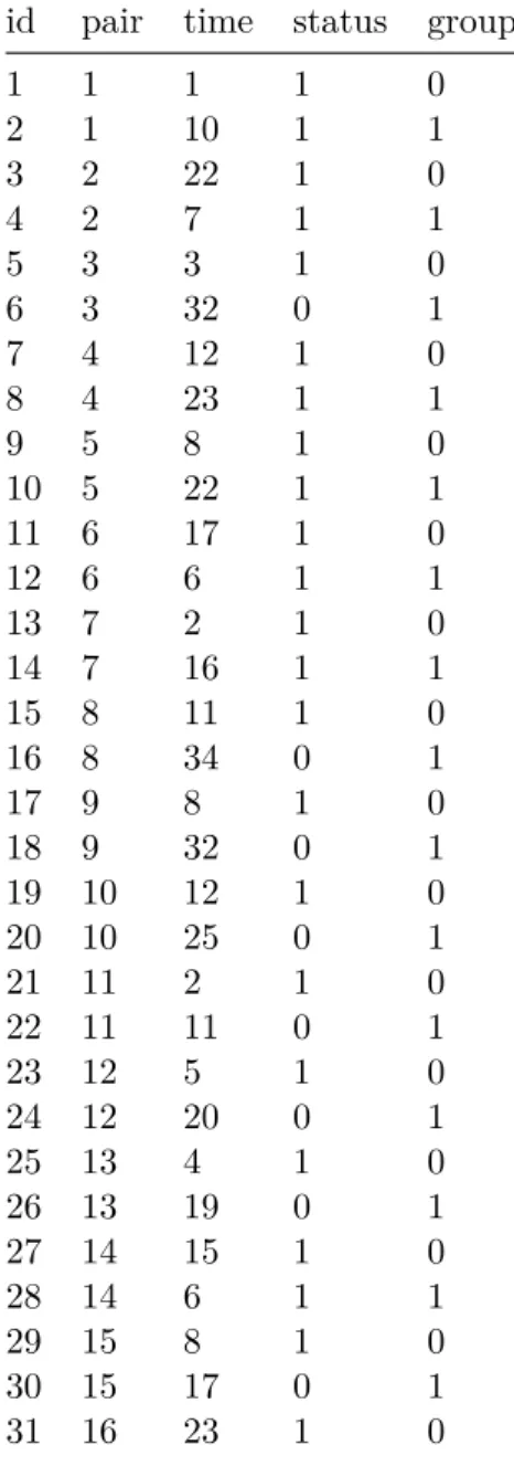
To set the scene, consider the survival data in Table 1.1. The data show the time (in weeks) from remission to relapse, hereinafter referred to as “survival time”, in two groups of acute leukemia patients initially treated with corticosteroids. A total of 42 patients, in complete or partial corticosteroid-induced remission, were randomly assigned at remission to one of two maintenance therapies: 6-MP, an immunosuppressive drug, or placebo. Patients were paired by remission status (complete or partial), a fact that we ignore for the moment. Details on the study design can be found in Gehan & Freireich (2011).

(17)

Table 1.1: The remission duration data. The first two columns contain the patient identification number and the pair identification number. The third column gives the time (in weeks) from remission to relapse (“survival time”) and the fourth column is the event indicator (1 = relapse, 0 = censored). The fifth column specifies the treatment group (1 = 6-MP, 0 = placebo).

id pair time status group

1 1 1 1 0 2 1 10 1 1 3 2 22 1 0 4 2 7 1 1 5 3 3 1 0 6 3 32 0 1 7 4 12 1 0 8 4 23 1 1 9 5 8 1 0 10 5 22 1 1 11 6 17 1 0 12 6 6 1 1 13 7 2 1 0 14 7 16 1 1 15 8 11 1 0 16 8 34 0 1 17 9 8 1 0 18 9 32 0 1 19 10 12 1 0 20 10 25 0 1 21 11 2 1 0 22 11 11 0 1 23 12 5 1 0 24 12 20 0 1 25 13 4 1 0 26 13 19 0 1 27 14 15 1 0 28 14 6 1 1 29 15 8 1 0 30 15 17 0 1 31 16 23 1 0

(18)

Chapter 1 7 32 16 35 0 1 33 17 5 1 0 34 17 6 1 1 35 18 11 1 0 36 18 13 1 1 37 19 4 1 0 38 19 9 0 1 39 20 1 1 0 40 20 6 0 1 41 21 8 1 0 42 21 10 0 1

1.2.1 Notations and terminology

The remission duration data is subject to right censoring. The survival

time random variable, i.e. time from randomisation (≈ time from

re-mission) to relapse is denoted by T. The censoring time, i.e. time from

randomisation to last contact in remission (study completion in this

case), is denoted byC. Therefore, the random variables that we observe

are Y = min(T, C) and ∆ = I(T ≤C), i.e. the follow-up time and the

event (relapse from remission) indicator. The realisations of (Y,∆) for

the remission duration data are given in columns 3 and 4 of Table 1.1. For example, patient 2 went out of remission at 10 weeks whereas obser-vation 42 is censored at the same time. Though not directly observed,

interest lies inT, the actual survival time. Besides the probability

den-sity functionf(·) and the cumulative distribution functionF(·), common

ways of characterising T are:

• the survival function

S(t) = Pr(T > t)

giving the probability that a patient continues to be in remission

(“survives”) at timet;

• the hazard function

h(t) = lim

∆t→0

Pr(t≤T < t+ ∆t|T ≥t) ∆t

giving the instantaneous rate at which relapses occur in time for patients still in remission;

(19)

• the cumulative hazard function H(t) =

Z t

0 h(v) dv

giving the total amount of risk accumulated from the start to the

present (t).

We have the following relationships between f(t), F(t), S(t), h(t),

and H(t): S(t) = 1−F(t) S(t) =−df dt(t) h(t) = f(t) S(t) S(t) = exp −H(t)

The density and survival functions ofC will be denoted byg(·) and

G(·), respectively.

1.2.2 Censoring

Coping with censored data requires working assumptions about the mechanism by which censoring occurs. A number of right censoring mechanisms, as well as other types of data incompleteness (e.g., interval censoring and truncation) are discussed in Lawless (2002, Chapter 2). The random right censorship model outlined above for the remission du-ration data (cf. Section 1.2.1) is adequate for most purposes. Further, it is typically required that the censoring mechanism is independent and non-informative. Under these conditions, a simple expression is obtained for the likelihood (see Section 1.2.3 below).

Independent censoring

Independent censoring is the requirement that the hazard rate of an at-risk subject coincides with the hazard rate in the surviving population, i.e. lim ∆t→₀ Pr(t≤T < t+ ∆t|T ≥t, C ≥t) ∆t = lim ∆t→0 Pr(t≤T < t+ ∆t|T ≥t) ∆t

(20)

Chapter 1 9

This requirement essentially means that the uncensored subjects under follow-up must be representative of the surviving population; a condi-tion that is satisfied when censoring occurs independently of the survival time (e.g., censoring due to calendar termination of the study). If there are covariates, then the independent censoring assumption is made con-ditional on the covariate information.

Non-informative censoring

If the censoring time distribution provides no information about the survival time distribution, then the censoring mechanism is said to be non-informative (for inference about the parameter(s) of interest). 1.2.3 Survival likelihood

With independent censoring, the joint distribution of T and C can be

factored into the product of the marginals. Therefore,

• (y,1) contributes to the likelihood with the factor f(y)G(y);

• (y,0) contributes to the likelihood with the factor S(y)g(y).

Further, if the censoring time distribution does not contain information on the parameter(s) of the survival time distribution (non-informative

censoring), then g(y) and G(y) can be dropped from the above

contri-butions. In that case,

• the relevant information contained in an event data is that the event occurred at the observed time;

• the relevant information contained in a censored data is that the event time exceeds the censoring time.

Under these conditions, the survival likelihood for a sample of size N is L∝ N Y j=1 f(yj)δjS(yj)1−δj = N Y j=1 h(yj)δjS(yj)

(21)

Note: independence assumption

As L is factored into the product of the individual data

contribu-tions, independence between observations is also required. 1.2.4 Kaplan-Meier survival curve

The Kaplan-Meier estimator is a non-parametric estimator of S(t).

Us-ing non-parametric maximum likelihood estimation ideas, the

Kaplan-Meier estimator treats T as a discrete random variable with probability

mass at the observed event times only (Kalbfleisch & Prentice, 2002, Section 1.4.1). Accordingly, the Kaplan-Meier survival curve is a (right continuous) step function with jumps at the event times. When there is no censoring, the Kaplan-Meier survival curve reduces to the empirical survival function.

The survival function at ˜y₍_j₎, thejth ordered event time, equals

S(˜y₍j)) = Pr T >y˜₍j) = Pr T >y˜₍j)|T >y˜(j−1) S(˜y₍j−1)) = j Y `=1 Pr T >y˜₍`)|T >y˜(`−₁₎

with ˜y₍₀₎ := 0. Under the assumption of independent censoring, the n`

subjects at risk for the event at ˜y₍`) are representative of the surviving

population at ˜y₍_`−₁₎ (since T is treated as discrete); cf. Section 1.2.2.

Therefore, the conditional probability in the above formula can be

esti-mated by the proportion of survivors in the sample at risk, i.e. (n`−d`)/

n`. Hence, by piecewise constant interpolation, the Kaplan-Meier

esti-mator takes the form ˆ

S(t) = Y

`: ˜y(`)≤t

n`−d`

n`

For a fixed t, the Kaplan-Meier estimator ˆS(t) has an asymptotic

normal distribution with mean S(t). The variance of ˆS(t) can be

esti-mated by Greenwood’s formula,

d Var ˆ S(t)=Sˆ(t)2 X `: ˜y(`)≤t d` n`(n`−d`)

(22)

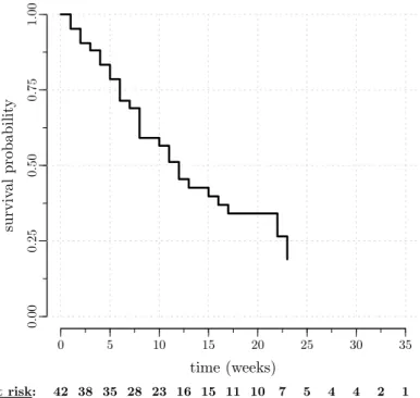
Chapter 1 11 0 5 10 15 20 25 30 35 time (weeks) surviv al probabil it y 0.00 0.25 0.50 0.75 1.00 at risk: 42 38 35 28 23 16 15 11 10 7 5 4 4 2 1

Figure 1.1: Kaplan-Meier survival curve in the remission duration data, with number of subjects at risk.

A plot of the Kaplan-Meier survival curve in the remission duration data is shown in Figure 1.1. The Kaplan-Meier survival curve crosses the 50% line at 12 weeks, the non-parametric estimate of the median survival time (i.e., the time beyond which the proportion in remission in

the study population equals 0.5). The value at the largest relapse time,

ˆ

S(23) = 0.189, is the proportion in remission at the end of the study.

When different from zero (i.e. when the last observation is a censored data), the Kaplan-Meier survival curve is undefined from that point on.

(23)

1.2.5 Weibull proportional hazards model

A popular distribution to model the survival time T is the Weibull

dis-tribution, with the following characteristics:

f(t) =λρtρ−1exp(−λtρ) F(t) = 1−exp(−λtρ) S(t) = exp(−λtρ) h(t) =λρtρ−1 H(t) =λtρ forρ >0 andλ >0.

A number of Weibull hazard functions are plotted in Figure 1.2. The Weibull hazard rate decreases, increases, or remains constant over

time for ρ < 1,ρ >1, or ρ = 1 (exponential distribution), respectively.

That is, ρ is a shape parameter. In contrast, the parameter λis a scale

parameter taking the form of a multiplier in the hazard function. Note: R syntax

The relation with the parametrisation used by dweibull()in R is

as follows

shape=ρ and scale=

1

λ

1/ρ

Weibull hazard rates with the same shape but different scales are proportional. Covariates that act on the Weibull scale parameter thus result in a proportional hazards model. The Weibull proportional haz-ards model for the remission duration data can be written as

h(t) =

(

λρtρ−1 in the placebo group

λexp(β)

ρtρ−1 in the 6-MP group

with exp(β) a summary measure of the effect of 6-MP therapy on the

relapse hazard rate (the exponential transformation ensures positivity without any parameter constraint).

By maximum likelihood estimation (cf. Section 1.2.3), we find ˆρ =

1.366 (se = 0.201), ˆλ= 0.046 (se = 0.026) and ˆβ=−1.731 (se = 0.413).

(24)

Chapter 1 13 0 2.5 5 0 1 2 λ= 1, ρ= 1.2 λ= 1, ρ= 1 λ= 1, ρ= 0.5 λ= 1.25, ρ= 1.2 time hazard rate

Figure 1.2: Weibull hazard functions.

indicates that 6-MP maintenance therapy reduces the risk of a relapse, and hence prolongs the duration of remission, in the study population.

The estimated hazard ratio is exp( ˆβ) = 0.177 (95% CI: [0.079,0.398]).

1.2.6 Cox model

Like the Weibull proportional hazards model (cf. Section 1.2.5), the Cox model specifies the way the explanatory variables act on the hazard rate, but, in contrast to the Weibull model, lets the time dependency of the hazard rate unspecified,

h(t) =h₀(t) exp(x0β)

with h₀(·) a non-specified baseline hazard function, x = (x₁ . . . xp)0

the vector of explanatory variables, and β = (β₁ . . . βp)0 the vector

of regression parameters. Owing to its semi-parametric nature, the Cox model has become routine in survival analysis. A nice and concise review can be found in Katz & Hauck (1993).

(25)

covariate information, say xj1 and xj2, is hj1(t) hj2(t) = exp (xj1 −xj2) 0 β

A one-unit change in one of the explanatory variables, while all other are kept fixed, results in a proportional change in the hazard function

(proportional hazards assumption). The parameterβkin the Cox model

is thus interpreted as a conditional log hazard ratio. In essence, the

proportionality assumption is the requirement that eachβk be constant

over time.

Ash₀(·) is left unspecified, we cannot make use of the survival

like-lihood from Section 1.2.3 to fit the Cox model. An estimate ˆβ ofβ can

be obtained by maximising a partial likelihood instead. Assuming no ties in the event times, the partial likelihood of the Cox model is given by (see, e.g., Klein & Moeschberger, 2003, Section 8.3)

Lp(β;Z) = N Y j=1 exp(x0_jβ) P `∈R(yj)exp(x 0 `β) !δj

with R(yj) the risk set at time yj containing all subjects still under

observation just prior to yj. The partial likelihood of the Cox model

can be derived as a profile likelihood obtained by maximising, for fixed

β, the survival likelihood with respect to the discretised version of the

baseline hazard function (Klein & Moeschberger, 2003, Section 8.3). In the case of ties, approximations of the partial likelihood (e.g., Breslow, Efron) can be used (Klein & Moeschberger, 2003, Section 8.4). Approx-imate standard errors of the maximum partial likelihood estApprox-imates are given by the square roots of the diagonal entries of the negative inverse

Hessian matrix of `p(·;Z) := log(Lp(·;Z)) evaluated at the maximum.

Even though Lp(·;Z) is not a genuine likelihood, it has been shown that

consistency and asymptotic normality properties for the estimator of β

are preserved (Gill, 1984).

In the remission duration data, we find (using the Breslow

approxi-mation to handle ties) exp( ˆβ) = 0.221 (95% CI: [0.099,0.493]).

1.3

Frailty model

In the remission duration data (Table 1.1), the response variable (time from remission to relapse) is observed for matched pairs of patients.

(26)

Chapter 1 15

Because of the matching, there is likely to be dependence in the data. Matched patients tend to be more alike than unmatched patients, thus indicating positive association within pairs. This kind of data is referred to as “clustered data”. In the remission duration data, clusters are of size 2. Multicentre clinical trial data, where patients are clustered within centres, typically involve larger and varying cluster sizes. The shared frailty model has been introduced to cope with clustered survival data.

For the jth subject (j = 1, . . . , ni) of the ith cluster (i = 1, . . . , s),

the (shared) frailty model is defined as

hij(t) =h0(t)uiexp(x0ijβ)

whereuidenotes the multiplicative effect of clusteri. Thus,uirepresents

the deviation of cluster i from the overall baseline risk. In the frailty

model, the cluster effect is random. That is, the ui’s are treated as the

actual (unobserved) values of a random variableU, the frailty term, and

hij(·) is interpreted as a conditional hazard givenU =ui.

The frailty term can be interpreted as an unobserved covariate

com-mon to, or shared by, individuals in a cluster. As U takes the same

value for each subject in a cluster, the frailty term generates (positive) association between event times in a cluster. The frailty model is based on a conditional independence assumption. Given the frailty and co-variates, observations are assumed to be independent. That is, if the common risk (frailty) term was known, observations would have been independent.

Another way to look at the frailty model is in terms of heterogeneity. Cluster heterogeneity, i.e. variation in susceptibility to the event from cluster to cluster, reflects different levels of risk across clusters and is modelled by the random variation of the frailty term. To put it dif-ferently, the presence of cluster heterogeneity indicates the presence of unknown risk factors varying from cluster to cluster. No cluster

hetero-geneity (U degenerated) implies independent data given the covariates,

and vice versa.

To model the frailty term, a distribution, called the frailty dis-tribution, is postulated. In principle, any distribution on the posi-tive half-line can play the role of the frailty distribution. To keep the mathematics tractable though, distributions with simple Laplace trans-forms are preferred. The Laplace transform of the frailty term, i.e.

L(x) = E exp(−U x)

(27)

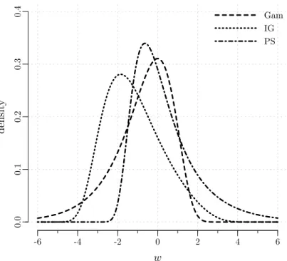
(provided that it exists) and plays an important role in frailty modelling. In the thesis appendix (Appendix 1), we describe, under the

parametri-sation that we shall use throughout the thesis†_{, the main characteristics}

of six important frailty distributions: the gamma (Gam), the inverse Gaussian (IG), the positive stable (PS), the log-normal (LN), the power variance function (PVF), and the compound Poisson (CP). The thesis appendix only collects useful formulas for ease of reference. The gen-eral characteristics of these frailty distributions are studied in detail in Hougaard (2000, Chapter 7) and in Duchateau & Janssen (2008, Chap-ter 4). In practice, the gamma distribution is most often used to model the frailty term.

The concept of shared frailty was introduced in Clayton (1978). Sug-gestions for introductory reading on this topic are Liang et al. (1995) and Hougaard (1995). A recent overview of frailty modelling is given in Govindarajulu et al. (2011). The frailty model methodology is thor-oughly presented in textbooks; see Hougaard (2000, Chapters 7–11), Duchateau & Janssen (2008), and Wienke (2010).

The latent nature of the frailty term makes it more difficult to fit frailty models. Inference for frailty models is discussed in Chapter 2. In practice, the most common way to fit the (gamma) frailty model is by

means of coxph() in R (part of the survival library). For a detailed

description of the proper use ofcoxph()for frailty models, see Therneau

& Grambsch (2000, Chapter 9).

In the remission duration data, we find (using coxph() with the

gamma frailty distribution and the Breslow approximation to handle

ties) exp( ˆβ) = 0.221 (95% CI: [0.099,0.493]). In this case, the frailty

model produces the same result as the Cox model. This suggests that the frailty term does not contribute to the model. Further indication is

provided by the estimated variance of the frailty term, ˆθ= 4.77×10−8_,

which is virtually zero.

Note: hij(·) :=h(· |xij, ui)

The notation hij(·) is used throughout the thesis as shorthand for

h(· |xij, ui), the conditional hazard for subjectj in clusteri.

†_{The densities are already rescaled to ensure identifiability of the parameters in the}

frailty model (Hougaard, 2000, page 221), similar to the zero-mean constraint for the random effects in the linear mixed model.

(28)

Part I

(29)

(30)

2 A unified framework for fitting the

frailty model with different frailty

distributions

There are at least three things that need to be put into consideration when it comes to choosing a method of estimation to fit the frailty model. The first one is a recurrent question in survival analysis: shall we specify a parametric form for the baseline hazard (parametric ap-proach) or shall we leave it unspecified (semi-parametric apap-proach)? A comparison of parametric and semi-parametric survival models can be found in Nardi & Schemper (2003). This chapter focuses on the para-metric approach. However, the results of this chapter are useful as well in the implementation of the EM algorithm within the semi-parametric setting. The second point concerns the choice of the frailty distribution. In this chapter, we show that many frailty distributions, including those introduced in the thesis appendix (Appendix 1), can be handled in a uniform way. Third, from a purely pragmatic point of view, software availability weighs in the balance. The method of this chapter, based on the maximum likelihood principle, only requires a numerical

optimi-sation procedure. We have implemented the method in the R library

parfm.

In Section 2.1, different likelihoods for frailty models are defined. The parametric frailty model is fitted based on the marginal likelihood. In Section 2.2, it is shown that a generic form of the marginal likelihood can be written by means of the derivatives of the Laplace transform of the frailty term. The parametric approach is outlined in Section 2.3. Ex-plicit derivative formulas are given in Section 2.4. Section 2.5 illustrates

the use of parfm.

For a detailed review of model estimation techniques in the semi-parametric setting, see Cortiñas Abrahantes et al. (2007). An overview of the available software in that setting is provided in Hirsch & Wienke

(31)

(2012).

The content of this chapter extends the results published in Munda et al. (2012).

2.1

Conditional, complete data, and marginal likelihoods

Observed data

LetZi be the vector that contains the relevant information from clusteri

(i= 1, . . . , s), i.e.

Zi =

n

(yij, δij,xij)|j= 1, . . . , ni

o

where yij is the time to event or censoring, whichever comes first, δij

indicates whether an observation corresponds to an event (δij = 1) or is

censored (δij = 0), and xij is the vector with the measured covariates

for subject j of clusteri. The frailty of cluster i,ui, is not observed.

Conditional likelihood

Given the latent data informationu= (u₁ . . . us)0 and the covariate

in-formation, event times are treated as independent (conditional

indepen-dence assumption). The conditional likelihood of the data Z={Zi|i=

1, . . . , s}is thus written as (cf. Section 1.2.3) Lcond(h0(·),β;Z|u) = s Y i=1 ni Y j=1 hij(yij) δij Sij(yij) =Ys i=1 ni Y j=1 h₀(yij)uiexp(x0ijβ) δij exp −H₀(yij)uiexp(x0ijβ)

Complete data likelihood

The complete data likelihood treats the frailties as if they were observed.

It therefore follows from the joint likelihood of Zand u,

(32)

Chapter 2 21

with f(·) := f(·;θ) the frailty density with parameter vector θ. If the

ui’s are independent and identically distributed, which we assume in the

following, then f(u) can be written asQs

i=1f(ui).

Marginal likelihood

To arrive at a likelihood not depending on the unobservables, the ui’s

have to be integrated out to form the marginal likelihood (also called the observed likelihood),

Lmarg(h0(·),β,θ;Z) = Z ∞ 0 · · · Z ∞ 0 Lfull(h0(·),β,θ;Z,u) du1· · ·dus (2.1) 2.2

Generic form of the marginal likelihood

It is convenient to rewrite the marginal likelihood (2.1) in a generic form

in terms ofL(·), the Laplace transform of the frailty termU, i.e. in terms

of

L(x) = Eexp(−U x)=

Z ∞

0 exp(−ux)f(u) du

Let Di = Pnj=1i δij denote the number of events in cluster i, and

L(q)₍_·_{) be the} _qth _{derivative of}_L₍_·_),_q_≥_{0, i.e.}

L(q)(x) = (−1)q Z ∞ 0 u q_exp(₋_ux₎_f₍_u_{) d}_u We have Lmarg(h0(·),β,θ;Z) = s Y i=1     ni Y j=1 h₀(yij) exp(x0ijβ) δij   × (−1)Di_L(Di)   ni X j=1 H₀(yij) exp(x0ijβ)    

(33)

Taking the logarithm, the marginal log-likelihood is obtained `marg(h0(·),β,θ;Z) = s X i=1     ni X j=1 δij log h₀(yij) +x0_ijβ   + log  (−1)DiL(Di)   ni X j=1 H₀(yij) exp(x0ijβ)       2.3 Parametric framework

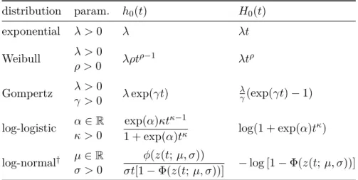
In the parametric framework, we adopt a baseline hazard function h₀(·)

that is completely specified, except for a number of unknown parameters

that are estimated together with β and θ. Common choices for h₀(·)

are collected in Table 2.1. This results in a fully parametric marginal log-likelihood that can be maximised by means of an optimisation rou-tine (e.g., a Newton-type algorithm). This task is most easily done

when L(q)₍_·_{) exists in closed form. This is the case for the gamma,}

the inverse Gaussian, the positive stable, the power variance function, and the compound Poisson frailty distributions (cf. Sections 2.4.1–2.4.5). The Laplace transform of a log-normal frailty term, on the other hand, does not exist in closed form. In that case, we can approximate the marginal log-likelihood by means of the Laplace approximation of inte-grals (cf. Section 2.4.6).

2.4

Derivative formulas

2.4.1 Gamma frailties

If U ∼Gam(θ), then the Laplace transform is

L(x) = (1 +θx)−1/θ

, x≥0

and, for q≥1, it is easy to see that

L(q)(x) = (−1)q(1 +θx)−q   q−1 Y `=0 (1 +`θ)  L(x)

(34)

Chapter 2 23

Table 2.1: Parametric baseline hazard and cumulative baseline hazard functions for selected event time distributions.

distribution param. h₀(t) H₀(t)

exponential λ >0 λ λt

Weibull λ >0 λρtρ−1 λtρ

ρ >0

Gompertz λ >0 λexp(γt) λ_γ(exp(γt)−1)

γ >0

log-logistic α∈R _{1 + exp(α)t}exp(α)κtκ−1_κ log(1 + exp(α)tκ)

κ >0

log-normal† µ∈R φ(z(t;µ, σ))

σt[1−Φ(z(t;µ, σ))] −log [1−Φ(z(t;µ, σ))]

σ >0 †_z

(t;µ, σ) :=(log(t)−µ)_/_σ_;_φ₍_·_{) and Φ(}_·_{) denote the density and the cumulative}

distribution functions of a standard normal random variable.

2.4.2 Inverse Gaussian frailties

If U ∼IG(θ), then the Laplace transform is

L(x) = exp 1 θ 1−√1 + 2θx , x≥0

and, for q≥1, we have (Munda et al., 2012)

L(q)(x) = (−1)q(2θx+ 1)−q/2 Kq−(1/2) _p 2θ−₁_(x₊₁_/₂_θ₎ K₁/2 _p 2θ−₁_(x₊₁_/₂_θ₎ L(x)

with Kγ(·) the modified Bessel function of the second kind,

Kγ(ω) = 1 2 Z ∞ 0 t γ−₁_exp₋ω 2 t+1 t dt, γ ∈R, ω >0

Alternatively, as IG(θ) = PVF(1, θ,1/2) (cf. Section 1.5 of the thesis

appendix), the formula of L(q)₍_x_{) from Section 2.4.4 can be used.}

2.4.3 Positive stable frailties

If U ∼PS(θ), then the Laplace transform is

(35)

and, for q ≥1, it is found in Wang et al. (1995) that (cf. Lemma 3.1 in that paper, which we write under a different parametrisation)

L(q)(x) = (−1)q(1−θ)x−θq   q−₁ X `=0 Ωq,q−`(θ) (1−θ)−`x−`(1−θ)  L(x)

where the Ωq,m(θ)’s are polynomials of degreeq−minθgiven recursively

by (cf. Appendix 2.A) Ωq,m(θ) =                  Γ q−(1−θ) Γ(θ) ifm= 1 Ωq−₁,m−₁(θ) + Ωq−1,m(θ)(q−1)−m(1−θ) ifm= 2, . . . , q−1 1 ifm=q

2.4.4 Power variance function frailties

If U ∼PVF(µ, θ, ν), then the Laplace transform is

L(x) = exp ( ν θ(1−ν) " 1− 1 +θµx ν 1−ν#) , x≥0

and, for q≥1, it is found in Hougaard (2000, Section A.3.4) that

L(q)(x) = (−1)q " q X `=1 Ωq,`(ν)µ`(1−ν) _ν θ `ν _ν θµ+x `(1−ν)−q# L(x)

where the Ωq,m(ν)’s are the same polynomials as above, evaluated at ν.

2.4.5 Compound Poisson frailties†

If U ∼CP(µ, θ, ν), then the Laplace transform has the same analytical form as for the PVF distribution (cf. Section 1.6 of the thesis appendix); therefore so are the derivatives.

†

(36)

Chapter 2 25

2.4.6 Log-normal frailties

IfU ∼LN(θ), then the Laplace transform does not exist in closed form.

Consequently L(q)₍_x_{) = (}₋₁₎qZ ∞ 0 u q_exp(₋_ux₎_f₍_u_{) d}_u = (−1)q_√1 2πθ Z ∞ 0 u q_exp(₋_ux₎1 uexp − 1 2θ log(u)2 du

needs to be approximated (x ≥ 0). By using the change of variable

w= log(u), we have L(q)(x) = (−1)q√1 2πθ Z ∞ −∞ exp(w)q exp −exp(w)xexp −w2 2θ ! dw = (−1)q√1 2πθ Z ∞ −∞exp ( qw−exp(w)x−w 2 2θ ) dw

We now show how to approximate this by means of the Laplace approx-imation of integrals. Let g(w;x, θ) :=−qw+ exp(w)x+w 2 2θ g(1)(w;x, θ) := dg dw(w;x, θ) =−q+ exp(w)x+ w θ g(2)(w;x, θ) := d 2_g dw2(w;x, θ) = exp(w)x+ 1 θ >0

The approximation consists of replacingg(·) by the first three terms

of its Taylor series expansion around some ˜w,

g(w;x, θ)≈g( ˜w;x, θ) + (w−w˜)g(1)( ˜w;x, θ) +(w−w˜)

2

2 g(2)( ˜w;x, θ)

The value of ˜w is chosen such that g(1)( ˜w;x, θ) = 0, so thatL(q)₍_x₎

can be approximated by L(q)₍_x₎_≈₍₋₁₎q _√1 2πθexp{−g( ˜w;x, θ)} × Z ∞ −∞exp ( −(w−w˜)2 2 g(2)( ˜w;x, θ) ) dw = (−1)q √1 θexp n −g( ˜w;x, θ)o hg(2)( ˜w;x, θ)i−1/2

(37)

where the last line follows by recognising the kernel of a normal density

with mean ˜wand variance 1/g(2)( ˜w;x, θ). This is known as the Laplace

approximation. The underlying idea is that the main contribution to

the integral comes from where g(·) is close to its minimum. We refer to

Goutis & Casella (1999) for further motivation and explanation of this kind of approximation.

Note: prediction of the frailty term

The explicit formulas for L(q)₍_·_{) are also useful to predict the value}

taken by the frailty term in a particular cluster. Indeed, the condi-tional expectation of the frailty term, given the observed data from

cluster iand the parameters, can be written as

E U|Zi;h0(·),β,θ = E UDi+1exp₋_UPni j=1H0(yij) exp(x 0 ijβ) EUDiexp −UPni j=1H0(yij) exp(x0ijβ) =− L(Di+1)Pni j=1H0(yij) exp(x 0 ijβ) L(Di) Pni j=1H0(yij) exp(x0ijβ)

which follows from applying Bayes’ formula to f(u|Zi;h0(·),β,θ).

In particular, predictions of the frailties are needed in the E-step of the EM algorithm (Nielsen et al., 1992).

The EM algorithm makes use of the complete data likelihood (cf. Section 2.1) to fit the frailty model in the semi-parametric setting. The algorithm iterates between an expectation step (or E-step) and a maximisation step (or M-step). In the E-step, the unobserved frailties are replaced by their conditional expectations given the observed data and the current parameter estimates. In the M-step, new parameter estimates are found by maximising the complete data likelihood, using the conditional expectations as offset terms.

(38)

Chapter 2 27

2.5

parfm†

The Rfunctionparfm(), part of the parfmlibrary, builds the marginal

log-likelihood and calls optim(), part of the stats library, to perform

the optimisation. The basic usage of parfm() (version 2.5.6) is as

fol-lows: Usage

parfm(formula, cluster, dist, frailty, data)

Arguments

formula a survival formula object

cluster character string indicating the cluster variable

dist character string indicating the baseline event time

distribution; one of "exponential", "weibull", "gompertz", "lognormal", "loglogistic"

frailty character string indicating the frailty distribution;

one of "gamma", "ingau", "possta", "lognormal"

data data frame containing the variables named in "formula"

and "cluster"

To illustrate parfm, we consider a litter-matched experiment studying

the effect of a drug on the time until the appearance of a tumour in rats (Mantel et al., 1977). Three (female) rats were chosen from each of 50 litters and followed for tumour incidence. Death from other causes was considered as a censoring event (73%). In each litter, one rat was selected at random and given the drug while the other two rats serve as

controls. In R, the data can be loaded using

> data(rats, package="survival")

> rats$time <− rats$time * 0.0328549 # days to months

> head(rats, n=10)

litter rx time status

1 1 1 3.318345 0 2 1 0 1.609890 1 3 1 0 3.416910 0 4 2 1 3.416910 0 5 2 0 3.351200 0 6 2 0 3.416910 0 7 3 1 3.416910 0 8 3 0 3.416910 0 9 3 0 3.416910 0 10 4 1 2.529827 0 †

(39)

Below are the results of running parfm() with different frailty distri-butions on the rats data, using the Weibull distribution to model the baseline hazard.

Gamma frailties > parfm(formula=Surv(time, status) ~ rx,

+ cluster="litter", dist="weibull", frailty="gamma",

+ data=rats)

Frailty distribution: gamma

Baseline hazard distribution: Weibull

Loglikelihood: −104.846 ESTIMATE SE p−val theta 0.489 0.469 rho 3.929 0.569 lambda 0.002 0.002 rx 0.907 0.322 0.005 ** −−− Signif. codes: 0 ’***’ 0.001 ’**’ 0.01 ’*’ 0.05 ’.’ 0.1 ’ ’ 1

Inverse Gaussian frailties > parfm(formula=Surv(time, status) ~ rx,

+ cluster="litter", dist="weibull", frailty="ingau",

+ data=rats)

Frailty distribution: inverse Gaussian Baseline hazard distribution: Weibull

Loglikelihood: −104.916 ESTIMATE SE p−val theta 0.541 0.647 rho 3.931 0.572 lambda 0.002 0.002 rx 0.911 0.323 0.005 ** −−− Signif. codes: 0 ’***’ 0.001 ’**’ 0.01 ’*’ 0.05 ’.’ 0.1 ’ ’ 1

Positive stable frailties

> # ‘iniFpar=’ sets the initial value of the frailty parameter (nu) > parfm(formula=Surv(time, status) ~ rx,

+ cluster="litter", dist="weibull", frailty="possta",

+ data=rats, iniFpar=0.4)

Frailty distribution: positive stable Baseline hazard distribution: Weibull

Loglikelihood: −104.947

(40)

Chapter 2 29 nu 0.094 0.095 rho 4.103 0.627 lambda 0.002 0.001 rx 0.944 0.327 0.004 ** −−− Signif. codes: 0 ’***’ 0.001 ’**’ 0.01 ’*’ 0.05 ’.’ 0.1 ’ ’ 1 Log-normal frailties > parfm(formula=Surv(time, status) ~ rx,

+ cluster="litter", dist="weibull", frailty="lognormal",

+ data=rats)

Frailty distribution: lognormal Baseline hazard distribution: Weibull

Loglikelihood: −104.599 ESTIMATE SE p−val sigma2 0.575 0.489 rho 3.963 0.576 lambda 0.002 0.001 rx 0.916 0.325 0.005 ** −−− Signif. codes: 0 ’***’ 0.001 ’**’ 0.01 ’*’ 0.05 ’.’ 0.1 ’ ’ 1

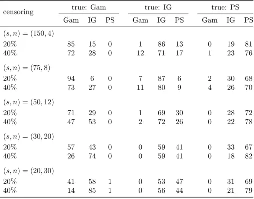
All models lead to a significant effect of the drug. Additionally, the treatment effect appears not to depend on the frailty distribution assumption, anticipating the properties of robustness discussed in Chap-ter 4.

In Klein & Moeschberger (2003, Section 13.3, Example 1.13) the re-sults are given for the semi-parametric gamma frailty model fitted with

the EM algorithm: ˆβ = 0.904 (se = 0.323) and ˆθ = 0.472 (se = 0.462).

These results are very close to the results obtained for the Weibull

gamma frailty model fitted with parfm.

Alternatively, the Weibull gamma frailty model can be fitted by

means of the frailtypacklibrary (Rondeau et al., 2012):

frailtypack fit > library(frailtypack)

> frailtyPenal(Surv(time, status) ~ rx + cluster(litter),

+ Frailty=TRUE, hazard="Weibull", data=rats)

Be patient. The program is computing ... The program took 0.77 seconds

Call:

frailtyPenal(formula = Surv(time, status) ~ rx + cluster(litter), data = rats, Frailty = TRUE, hazard = "Weibull")

(41)

Shared Gamma Frailty model parameter estimates using a Parametrical approach for the hazard function

coef exp(coef) SE coef (H) z p

rx 0.90751 2.47814 0.322339 2.81539 0.0048718

Frailty parameter, Theta: 0.488854 (SE (H): 0.469033 )

marginal log−likelihood = −241.47

AIC = Aikaike information Criterion = 1.63648

The expression of the Aikaike Criterion is:

’AIC = (1/n)[np− l(.)]’

Scale for the weibull hazard function is : 140.91 Shape for the weibull hazard function is : 3.93 The expression of the Weibull hazard function is:

’lambda(t) = (shape.(t^(shape−1)))/(scale^shape)’

The expression of the Weibull survival function is:

’S(t) = exp[− (t/scale)^shape]’

n= 150

n events= 40 n groups= 50

(42)

Chapter 2 31

Appendix 2.A

The Ωq,m(·)’s polynomials

The Ωq,m(·)’s that appear in L(q)(·) for the positive stable, the power

variance function, and the compound Poisson frailty distributions are

polynomials of degree q−m inα given recursively by

Ωq,m(α) =                  Γ q−(1−α) Γ(α) ifm= 1 Ωq−₁,m−₁(α) + Ωq−₁,m(α)(q−1)−m(1−α) ifm= 2, . . . , q−1 1 ifm=q forα∈(0,1).

The first few polynomials are

m= 1 m= 2 m= 3 m= 4             q= 1 1 q= 2 α 1 q= 3 α(α+ 1) 3α 1 q= 4 α(α+ 1)(α+ 2) 7α2+ 4α 6α 1

An Rfunction to calculate the Ωq,m(α)’s for q = 1, . . . , Q is

Omega <− function(Q, alpha)

{ # Q = order of the derivative > 0, alpha in (0, 1)

Omega <− matrix(NA, nrow=Q, ncol=Q, dimnames=list(q=1:Q, m=1:Q))

diag(Omega) <− 1 if(Q < 2) return(Omega) Omega[q=2:Q, m=1] <− cumprod(alpha + 0:(Q − 2)) if(Q < 3) return(Omega) for(m in 2:(Q− 1)) for(q in (m + 1):Q) Omega[q, m] <− Omega[q − 1, m− 1] + Omega[q− 1, m] * ((q − 1) − m * (1− alpha)) return(Omega) } For example,

(43)

> Omega(Q=4, alpha=0.1) m q 1 2 3 4 1 1.000 NA NA NA 2 0.100 1.00 NA NA 3 0.110 0.30 1.0 NA 4 0.231 0.47 0.6 1 Appendix 2.B Derivative formulas in R Gamma frailties

Lq_Gam <− function(q, theta, x)

{ # q >= 0, theta > 0, x >= 0 if(q == 0){

(1 + theta * x)^(−1 / theta)

} else{

(−1)^q * (1 + theta * x)^(−q) * prod(1 + 0:(q− 1) * theta) *

Lq_Gam(q=0, theta=theta, x=x) }

}

Inverse Gaussian frailties

Lq_IG <− function(q, theta, x)

{ # q >= 0, theta > 0, x >= 0 if(q == 0){

exp((1− sqrt(1 + 2 * theta * x)) / theta)

} else{

z <− theta^(−0.5) * sqrt(2 * x + 1 / theta)

(−1)^q * (2 * theta * x + 1)^(−q / 2) *

besselK(x=z, nu=q − 0.5) / (sqrt(0.5 * pi / z) * exp(−z)) *

Lq_IG(q=0, theta=theta, x=x) }

}

Positive stable frailties

Lq_PS <− function(q, theta, Omega, x)

{ # q >= 0, theta in (0, 1), x >= 0 if(q == 0){ exp(−x^(1− theta)) } else{ Sum <− 0 for(l in 0:(q − 1)){ Sum <− Sum +

(44)

Chapter 2 33

}

(−1)^q * ((1− theta) * x^(−theta))^q * Sum *

Lq_PS(q=0, theta=theta, x=x) }

}

Power variance function & compound Poisson frailties

Lq_PVF <− function(q, mu, theta, nu, Omega, x)

{ # q >= 0, mu > 0, theta > 0, nu in (0, 1) (PVF) or nu > 1 (CP), # x >= 0

if(q == 0){

exp(nu / (theta * (1 − nu)) *

(1 − (1 + theta * mu * x / nu)^(1− nu)))

} else{

Sum <− 0

for(l in 1:q){

Sum <− Sum +

Omega[q, l] * mu^(l * (1− nu)) * (nu / theta)^(l * nu) *

(nu / (theta * mu) + x)^(l * (1− nu)− q)

}

(−1)^q * Sum * Lq_PVF(q=0, mu=mu, theta=theta, nu=nu, x=x)

} } Log-normal frailties Lq_LN <− function(q, theta, x) { # q >= 0, theta > 0, x >= 0 g <− function(w, q, x, theta) −q * w + exp(w) * x + 0.5 * w^2 / theta options(warn=−1)

wTilde <− nlm(f=g, p=0, q=q, theta=theta, x=x)$estimate

options(warn=0)

(−1)^q * theta^(−0.5) * exp(−g(w=wTilde, q=q, x=x, theta=theta)) *

(exp(wTilde) * x + theta^(−1))^(−0.5)

(45)

(46)

3 A diagnostic plot for the frailty

distribution in the shared frailty model

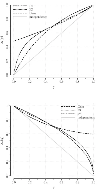
When modelling dependence between event times, not only the degree of global dependence is of interest, but also the way the local (at a given time) dependence changes over time, i.e. the dependence structure. In particular, the times at which the dependence is high often receive special attention (see, e.g., Nan et al., 2006).

In the frailty model framework, the dependence structure is dic-tated by the frailty distribution (Anderson et al., 1992; Hougaard, 1995). Hence, the frailty distribution needs to be carefully chosen to correctly model the dependence structure in the data. As the frailties are un-observed, though, specifying the frailty distribution is a difficult issue. This chapter introduces a new diagnostic plot to guide the choice of the frailty distribution.

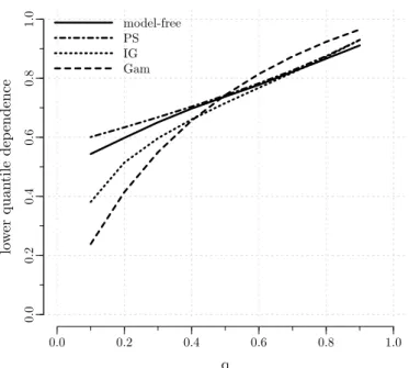
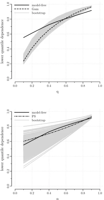
Section 3.1 provides references to key papers in the area and out-lines a general diagnostic framework based on dependence measures. In Section 3.2, we review common ways to measure dependence in survival data and we discuss the patterns of dependence induced by different frailty distributions. From the discussion of Section 3.2, it will become clear that the probability mass that a frailty distribution puts in the tails is a key feature as it drives the dependence structure. To cap-ture the behaviour in the tails, the proposed diagnostic plot is based on the quantile dependence function. Quantile dependence is introduced in Section 3.3 where we explain how to obtain the model-based and the non-parametric estimates that are used to construct the diagnostic plot. The method is illustrated in Section 3.4 and is assessed with simulations in Section 3.5. Concluding remarks are given in Section 3.6.

The content of this chapter is submitted for publication (Munda & Legrand, 2014b).

(47)

3.1

Introduction

As a matter of software availability, the gamma distribution is often used in practice to model the frailty term. Diagnostic checks specific to the gamma frailty distribution include Shih & Louis (1995), Cui & Sun (2004), and Geerdens et al. (2013). Only a few diagnostic procedures are available for other frailty distributions. The graphical tool developed in

Economou & Caroni (2008) is valid if, for all t, the distribution of the

frailty term among the “surviving clusters” at timetbelongs to the same

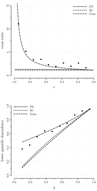
family as the original frailty distribution (closure property). In Oakes (1989), the cross ratio function, a measure of bivariate dependence, is used as a diagnostic tool. The method can in principle be used with any frailty distribution, but does not explicitly account for censoring. Some technical improvements of the method are proposed in Viswanathan & Manatunga (2001) and in Chen & Bandeen-Roche (2005). Another, more computationally demanding, diagnostic tool based on the cross ratio function is studied in Glidden (2007).

In the last four papers cited above, the basic idea is that although frailties are unobservable, the dependence structure that they impose on the data can be observed. Further, the dependence structure is dictated by the frailty distribution (Anderson et al., 1992; Hougaard, 1995). It fol-lows that a graphical comparison of the observed dependence structure with selected model-based structures can be used to reveal the frailty distribution that best describes the pattern of dependence in the data. That is, the problem of assessing the frailty distribution assumption can be linked to the problem of measuring dependence in clustered survival data. Common ways to measure dependence in clustered survival data are reviewed in the next section.

3.2

Dependence in bivariate survival data

Dependence measures have been developed mainly for bivariate data. In this section, we review a number of coefficients that evaluate dependence

(48)

Chapter 3 37

3.2.1 Overall dependence

Kendall’s τ is a rank-based dependence coefficient which ranges from

−1 to 1, with τ = 0 under independence. To define Kendall’s τ, we

need an independent copy (i.e. with the same distribution) of (T₁, T₂),

say (T₁0, T₂0). Kendall’s τ is the probability that (T₁, T₂) and (T₁0, T₂0) are

concordant minus the probability that this pair is discordant, τ = Pr(T₁−T₁0)(T₂−T₂0)>0−Pr(T₁−T₁0)(T₂−T₂0)<0

Thus, Kendall’s τ expresses the probability that the order of the first

coordinates is the same as the order of the second coordinates (“con-cordance”, i.e. large values tend to occur with large values and small values tend to occur with small values) minus the probability that the

order differs between the coordinates (“discordance”). Kendall’s τ is

scale-invariant, i.e. it remains unchanged under monotonic transforma-tions of the random variables. It is worth noting that interpretation of

Kendall’s τ requires a pair of clusters and that observations within a

cluster must have an ordering ((T₁ −T₁0)(T₂ −T₂0) is not the same as

(T1−T₂0)(T₂−T₁0)).

An alternative to Kendall’s τ, which can be interpreted with one

cluster only, is given by the median concordance coefficient, also known

as Blomqvist’sβ,

β= Pr(T₁−˜t₁)(T₂−˜t₂)>0−Pr(T₁−˜t₁)(T₂−˜t₂)<0