Modeling Interest Rate Parity: A System Dynamics
Approach
John T. Harvey
Department of Economics Texas Christian University
Working Paper Nr. 05-01
September 2005
Department of Economics Texas Christian University P.O. Box 298510 Fort Worth, TX 75087 www.econ.tcu.edu
Texas Christian University
Texas Christian University
Texas Christian University
Texas Christian University
Department of Economics
Department of Economics
Department of Economics
Department of Economics
Modeling Interest Rate Parity: A System Dynamics Approach
John T. Harvey Professor of Economics Department of Economics
Box 298510 Texas Christian University Fort Worth, Texas 76129
(817)257-7230 j.harvey@tcu.edu
Presented at the Association for Evolutionary EconomicsConference
Modeling Interest Rate Parity: A System Dynamics Approach
The theory of uncovered interest rate parity has enjoyed very little empirical support. Despite the fact that global financial markets trade seven days a week, twenty-four hours a day and
communication takes place almost instantaneously, there are strong indications that differences in expected rates of return across countries can be non-zero and large for extended periods of time.
However, these deviations display a pattern within which there is an important clue regarding their cause. Changes in the differences between expected rates of return across countries largely
correspond to changes in the differences between national interest rates. In other words, when
agents expect the rate of return (taking into account both interest rates and forecast exchange rate movements) to be higher in one country than another, that country also tends to have the higher interest rates. This means, as will be demonstrated below, that deviations from uncovered interest rate parity cannot be explained (as has been argued elsewhere) by relying on the assumption that agents perceive some assets to be riskier than others. A model of international financial flows that incorporates John Maynard Keynes’ concept of forecast confidence, however, has no difficulty explaining this commonly observed phenomenon.
The purpose of this paper is to show the superiority of Keynes’ approach by comparing three system dynamics models of the relationship among interest and exchange rates: one based on traditional uncovered interest rate parity, one with risk, and one with forecast confidence. It will be demonstrated that only the last produces patterns consistent with those observed in the real world. This paper is an extension of the empirical study undertaken in Harvey (2004).
Uncovered Interest Rate Parity
Uncovered interest rate parity makes the seemingly innocuous claim that the return on interest-bearing assets throughout the world must be identical once expected exchange rate movements are taken into account. This can be expressed (using the dollar and the euro to make the example more concrete) as shown in equation (1):
(1) (1+r$) = (i/$)(1+ri)($/i)e
where r$ is the rate of interest paid on dollar deposits, ri is the rate of interest paid on euro deposits,
(i/$) is the spot price of dollars in euros, and ($/i)e is the market’s expectation of the spot price of the
euro (in dollars) at some future date (where the time horizon of the interest rates and the exchange rate expectation are the same). If one side exceeds the other it is then assumed that this sets into motion forces that will restore the equilibrium. Were the left side of (1) to exceed the right side, for example, this would create capital flows from the euro to the dollar, driving r$ down (as capital becomes less
scarce), ri up (as capital becomes more scarce), and (i/$) up (as agents buy the dollar with the euro,
causing the former to appreciate).
Figure 1 shows a system dynamics model (written in Vensim) of the basic uncovered interest rate parity relationship introduced in equation (1). At the center is UIRP Deviation, which is measured
as (1+r$) - (i/$)(1+ri)($/i)e (i.e., the amount by which the market expects that US returns will
exceed foreign). If this number is zero, equilibrium prevails and nothing is transmitted along the single arrow emanating from UIRP Deviation. If instead, for example, US returns are expected to be greater
than those of foreign assets, this will lead to a rise US Net Capital Inflows (hence the positive sign on
the arrow linking UIRP Deviation and US Net Capital Inflows). This affects three variables in the
FX per USD Delta FX per USD
Expected FX per USD UIRP Deviation -+ Market Forces US Interest Rate Foreign Interest Rate -Delta Foreign Interest Rate Delta US Interest Rate US Net Capital Inflows + -+ US Financial Mkt Foreign Financial Mkt Currency Market US Central Bank Policy Adjustment US Interest Rate + + + +
Figure 1: Traditional UIRP model without risk or forecast confidence.
sign on the arrow; more on the construction of this variable below), the Foreign interest rate (which
rises as capital becomes more scarce–note the positive sign), and FX per USD, or units of foreign
currency per dollar (this rises as agents buy the dollar in order to buy US interest-bearing assets; note the positive sign). I chose to model the exchange rate and the two interest rates as levels affected by rates. Delta on each is the amount by which the US Net Capital Inflows caused a change in this time
period. Expected FX per USD is treated as exogenous, and FX per USD, Expected FX per USD,
Foreign interest rate, and US interest rate feed back into UIRP Deviation so as to solve for the
Note that US Interest Rate is affected by an exogenous force and an endogenous one. US
Interest Rate is simply the sum of Market Forces US Interest Rate (whose construction is parallel to
that of Foreign Interest Rate) and US Central Bank Policy Adjustment. This was done so that
external shocks to the interest rate could be introduced through the latter. An equivalent policy variable for Foreign Interest Rate was not created since US Central Bank Policy Adjustment is sufficient to
create changes in interest rate differentials.
I chose to measure the interest rates as decimal numbers (0.06 for 6%, for example) and the exchange rates (both actual and expected) as indices beginning with 100. To give a sense of the behavior the parameters and starting values create, suppose we start with model with FX per USD =
100, Expected FX per USD = 100, Foreign interest rate = 0.06, and US interest rate = 0.06. In
that case, UIRP Deviation = 0 and the model sits in equilibrium (generating a flat line at zero for UIRP
Deviation). To throw the model out of equilibrium, introduce a US Central Bank Policy Adjustment
of -0.04, temporarily lowering US Interest Rate to 0.02. This means that there is now a UIRP
Deviation of -0.04, causing agents expect US interest-bearing assets to earn (once exchange rate
movements are taken into account) a 4% lower return than foreign ones.
The first consequence of this change is that the arrow from UIRP Deviation to US Net
Capital Flows now carries a non-zero signal. As I chose to measure the latter as a simple index
wherein net capital flows would be equal to 100 times the deviation, US Net Capital Flows are now
-4 (-0.0-4 times 100). The --4 is carried out in three separate directions. In terms of the impact of capital flows on interest rates, I opted to have 10% of any given deviation be corrected per round (which represents one hour). For example, when the -4 is fed into Delta US Interest Rate, it is multiplied by
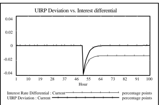
UIRP Deviation vs. Interest differential 0.04 0.02 0 -0.02 -0.04 2 2 2 2 2 2 2 2 2 2 2 2 2 2 2 1 1 1 1 1 1 1 1 1 1 1 1 1 1 1 1 10 19 28 37 46 55 64 73 82 91 100 Hour
Interest Rate Differential : Current 1 1 1 1 1 1 percentage points UIRP Deviation : Current 2 2 2 2 2 2 2 percentage points
Figure 2: Traditional UIRP, pattern of UIRP deviation compared to
interest rate differential.
deviation. Meanwhile, the -4 is multiplied by 0.001 in Delta Foreign Interest Rate, so that the
adjustment is also 0.4% (albeit in the other direction), again 1/10 of the deviation. With respect to the exchange rate, there the -4 is multiplied by 0.1, meaning that (since the initial value for FX per USD is
set at an index of 100) it falls to 99.6. This, too, is 1/10 of the way back to equilibrium (the value of FX per USD that would eliminate the deviation is 96.2, or roughly 96). With these values and
parameters it requires 41 hours for the system to return to equilibrium at UIRP Deviation = 0 (the use
of hours as the time period does not affect the behavior of the model; one could imagine this as minutes, instead).
Figure 2 shows what was described above (ignore “Interest Rate Differential” for the moment). In periods 1 through 50, Foreign Interest Rate = US Interest Rate = 0.06 and FX per USD =
Expected FX per USD = 100. Therefore, UIRP Deviation = 0 and simulation is flat at that value. In
period 51, however, there is a US Central Bank Policy Adjustment of -0.04, so that the US Interest
Rate falls to 0.02. This lowered UIRP Deviation to -0.04, but the adjustment begins immediately. It is
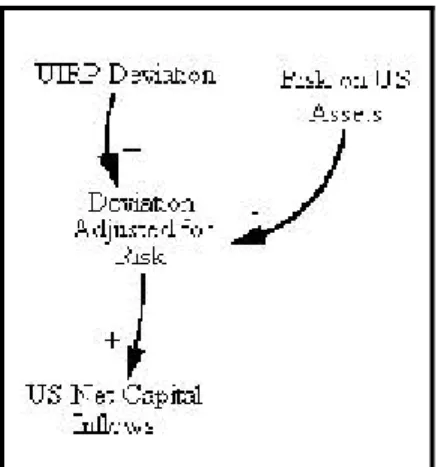
Figure 3: Link from UIRP Deviation to US Net Capital Inflows, adjusted for risk.
Returning to the thesis of this paper, the key issue is whether or not changes UIRP Deviation
tend to mimic those of the simple interest rate differential, US Interest Rate minus Foreign Interest
Rate. The plot of the interest rate differential in Figure 2 offers evidence to the contrary, the particular
problem being the behavior of UIRP Deviation. One can temporarily throw it out of equilibrium, as
occurs at hour 51, and in a manner that is consistent with real-world observations (i.e., UIRP
Deviation and the interest rate differential move in the same direction and both are, in this case,
negative). But UIRP Deviation soon returns to zero. We do not see the model settling into an
equilibrium wherein UIRP Deviation and the interest rate differential are both non zero and of the same
sign. Traditional interpretations of UIRP cannot account for the patterns observed in the real
world because UIRP Deviation must always return to zero.
A common (and reasonable) modification of UIRP is to add risk. This is accomplished by intercepting the signal from UIRP Deviation to US Net Capital Flows and altering it to reflect agents’
concerns about the assets of a particular country. The modification to Figure 1 is illustrated in Figure 3 (to save space just the change is shown–the rest of the model
is identical to that shown in Figure 1). Risk on US Assets is
measured in decimal form and represents the premium that US asset issuers must pay in order to convince agents to hold them despite their greater risk. This number is then subtracted from UIRP Deviation in Deviation Adjusted for Risk to
create the value that affects US Net Capital Flows.
Figure 4 shows the plot of model with the adjustment for risk. The behavior is the same as that shown in Figure 2 but, because of the 0.02 risk premium on US assets, UIRP Deviation is drawn
UIRP Deviation vs. Interest Differential 0.06 0.04 0.02 0 -0.02 2 2 2 2 2 2 2 2 2 2 2 2 2 2 2 1 1 1 1 1 1 1 1 1 1 1 1 1 1 1 1 10 19 28 37 46 55 64 73 82 91 100 Hour
Interest Rate Differential : Current 1 1 1 1 1 1 1 1 1 1
UIRP Deviation : Current 2 2 2 2 2 2 2 2 2 2 1
Figure 4: Traditional UIRP with risk, pattern of UIRP deviation
compared to interest rate differential.
toward 2% rather than 0% (note that I started the model with US Interest Rate at 0.08 rather than
0.06 so that this simulation would begin in equilibrium). When the US Central Bank Policy
Adjustment becomes -0.04 in hour 51, UIRP Deviation settles at 2% and the interest rate differential
returns to equilibrium at -1.36%. UIRP Deviation and the interest rate differential are both non zero,
but they are the opposite sign. The key of course is that regardless of what we introduce with respect to the interest rate differential, UIRP Deviation must always return to 2% (or whatever value we
select) because it simply reflects the risk premium on US assets. Depending on the shocks we
introduce into the system, interest rate differential can come to rest at a number of different values;
UIRP Deviation, however, will inevitably find its equilibrium at 2%. Since there is no reason to
assume that the risk premium will invariably be the same sign as the simple interest rate differential (though it can by coincidence), this approach also comes up short in terms of generating patterns consistent with what we observe in the real world.
Modifying the model according to the observations made by John Maynard Keynes in the
General Theory (1964; see especially chapter twelve), however, yields an approach that is perfectly
consistent with empirical observations. There, he argues that agents’ confidence in their forecasts is an important and overlooked consideration. Recall the construction of UIRP Deviation. All of the
component variables are known by market participants to be accurate except one: Expected FX per
USD. It is necessarily a forecast, and an extremely important one given the potential for substantial
exchange rate movements over the time horizon in question.
So, by virtue of the fact that Expected FX per USD is one of its components, UIRP
Deviation is a forecast, and forecasts are never certain. In general, the more confidence agents have in
their predictions, the more funds they are willing to commit in speculation. The most realistic way to incorporate this into the model would be to make capital flows (for a given UIRP Deviation) go from a
trickle to a strong flow as forecast confidence increased. To make the exposition simple, however, I elected instead to let portfolio investment flow either unimpeded or not at all depending on whether the absolute value of UIRP Deviation exceeded a critical value. I modeled the latter as an inverse function
of market confidence and expressed it as a forecast error. For example, market participants may expect a UIRP Deviation of 0.03, but with an anticipated forecast error of +/-0.02. In other words,
they believe that the return on U.S. interest-bearing assets will be 3%, though they would not be surprised if it were as low as 1% (i.e., 3%-2%) or as high as 5% (i.e., 3%+2%).
I then supposed a simple rule of thumb for agents in the model: whenever the absolute value of the UIRP Deviation exceeds the absolute value of Forecast Error, agents should unhesitatingly buy
the assets of the nation with the higher expected return (and capital flows unabated). This is so because even under the worst-case scenario one still profits. On the other hand, when the absolute value of the
Figure 5: Link from UIRP Deviation to US Net Capital Inflows, adjusted for confidence.
(and no capital will flow) since within the range of possible outcomes includes one that yields a loss. Again, this is a simplification over a specification that would allow for ranges of capital flow (from unhindered to zero), but it will be much simpler to model and still give the same basic result.
Figure 5 shows the adjustment to Figure 1 necessary to incorporate Keynes’ confidence (it is possible to combine risk and confidence in the same model; I opted not to do so for simplicity and because it does not alter the results). Note that, unlike in the rest of the exposition, the signs on the arrows feeding into Trigger Point Determination are based on the absolute values of UIRP
Deviation and Forecast Error. The arrow from Trigger Point Determination to US Net Capital
Flows is in a sense simply a continuation of that from UIRP Deviation, the only difference being that if
UIRP Deviation does not exceed Forecast Error, azero signal be
sent to US Net Capital Flows. Otherwise, the behavior is exactly as
explained for Figure 1 and Trigger Point Determination has no
effect on the signal from UIRP Deviation at all.
Figure 6 shows the same scenario as set out in Figures 2 and 4, but with confidence explicitly modeled. The forecast error is set at 1%, such that agents, for a given UIRP Deviation, believe that their
forecast will fall within one percentage point of that value, plus or minus.
UIRP Deviation vs. Interest Differential
0.04 0.02 0 -0.02 -0.04 2 2 2 2 2 2 2 2 2 2 2 2 2 2 2 1 1 1 1 1 1 1 1 1 1 1 1 1 1 1 1 10 19 28 37 46 55 64 73 82 91 100 DayInterest Rate Differential : Current 1 1 1 1 1 1 1 1 1 1 UIRP Deviation : Current 2 2 2 2 2 2 2 2 2 2 1
Figure 6: UIRP with Keynes’ confidence, pattern of UIRP Deviation compared to interest
rate differential.
Finally, we observe what is commonly seen in the real world: UIRP Deviation moves with the
raw interest rate differential. Both settle into equilibrium at negative values, with the interest rate differential at -2.06% and UIRP Deviation at -1%. That the latter comes to rest at this level is a
function of the fact that Forecast Error is 1%; capital will flow (and variables adjust) only when UIRP
Deviation > Forecast Error; once UIRP Deviation is less than or equal to Forecast Error, the flow
stops and hence the adjustment in UIRP Deviation stops. Figure 7 shows the same setup with multiple
shocks to US Interest Rate ( US Central Bank Policy Adjustment is 0 in periods 1-24, 0.04 from
25-50, 0 from 51-75 and -0.04 from 76-100). Again, UIRP Deviation adjusts only up to the point
that it is less than or equal to Forecast Error (1% in this example) in absolute value. The reader
UIRP Deviation vs. Interest Differential
0.04 0.02 0 -0.02 -0.04 2 2 2 2 2 2 2 2 2 2 2 2 2 2 2 1 1 1 1 1 1 1 1 1 1 1 1 1 1 1 1 10 19 28 37 46 55 64 73 82 91 100 DayInterest Rate Differential : Current 1 1 1 1 1 1 1 1 1 1 UIRP Deviation : Current 2 2 2 2 2 2 2 2 2 2 1
Figure 7: UIRP with Keynes’ confidence, pattern of UIRP Deviation compared to interest
rate differential with multiple shocks.
differential are not of the same sign in this specification, but, just as in the real world, it is the exception rather than the rule. In general, because agents lack the conviction to completely trust their exchange rate forecasts, UIRP Deviation is pulled in the direction of the raw interest rate movements and the
subsequent deviation is not completely eliminated.
Conclusion
The empirical failure of uncovered interest rate parity has stood as a mystery for a very long time in financial economics. Attempts to solve the problem using risk have failed time and again. Reaching back to Keynes, however, offers a solution that is both up to the task and intuitively appealing. A realistic formulation of agents’ expectations (a variable, incidentally, to which very little attention has been paid up to this point) suggests that what we conclude from the standard approach to
REFERENCES
Harvey, John T. “Deviations from uncovered interest rate parity: a Post Keynesian explanation.”
Journal of Post Keynesian Economics 27, no.1 (Fall 2004): 19-36.
Keynes, John Maynard. The General Theory of Employment, Interest, and Money. New York: