Clemson University Clemson University
TigerPrints
TigerPrints
All Theses Theses
August 2020
Training a Camera Based Inspection System for Appearance
Training a Camera Based Inspection System for Appearance
Variability
Variability
Vihang KhareClemson University, [email protected]
Follow this and additional works at: https://tigerprints.clemson.edu/all_theses
Recommended Citation Recommended Citation
Khare, Vihang, "Training a Camera Based Inspection System for Appearance Variability" (2020). All Theses. 3397.
https://tigerprints.clemson.edu/all_theses/3397
TRAINING A CAMERA-BASED INSPECTION SYSTEM
FOR APPEARANCE VARIABILITY
A Thesis Presented to the Graduate School of
Clemson University In Partial Fulfillment
of the Requirements for the Degree Master of Science
Computer Engineering by
Vihang Yashodhan Khare August 2020
Accepted by:
Dr. Adam Hoover, Committee Chair Dr. Richard Brooks
Abstract
This thesis considers the problem of variability in the appearance of machine parts while performing automated camera-based inspections in an appliance manu-facturing plant. In an appliance manumanu-facturing plant, machine parts are inspected to find any defects which might have occurred while assembling them. Training the system for the different appearances of these parts is important for detecting defects with high accuracy and precision. Machine parts have a lot of variability in their ap-pearance and it is a difficult and time consuming task to train the inspection system for the same. Previously, a tool (clustering) was developed by our group that could automatically learn the different appearances of machine parts that needed inspec-tion [7]. In this thesis, we perform different experiments using the tool with a goal of training an inspection system prototype for the learned variability. To do our exper-iments, we collected a total of 249,371 images for 9 inspection problems. A manual review of the data identified a range of 2-180 defects per problem. Our inspection system prototype, post training, achieved a range of 83% - 100% defect detection with a range of 0.0-2.9 false alarms per defect for 8 out of the 9 inspection problems. One of inspection problems was not firm in its structure, and in our experiments we could only find 50 % of the defects with a false alarms per defect rate of 5.0. Based on these results, we have designed a decision tree that could be used by engineers for training an inspection system for new inspection problems, for appearance variability.
Acknowledgments
I would like to thank my advisor, Dr. Adam Hoover and the entire department of Electrical and Computer Engineering at Clemson University for this wonderful opportunity. Working on this project has been the best learning experience of my life, both, personally and professionally. I feel it is a huge stepping stone to my career. I would also like to thank the team at Samsung, especially Ravee Vaid-hyanathan and Anatole Figueroa. Their guidance was critical for helping us collect and interpret data.
Table of Contents
Title Page . . . i
Abstract . . . ii
Acknowledgments . . . iii
List of Tables . . . vi
List of Figures . . . vii
1 Introduction . . . 1
1.1 Camera-based inspection system . . . 2
1.2 Part appearance variability . . . 4
1.3 Training for part appearance variability . . . 5
1.4 Background . . . 9 1.5 Related Work . . . 24 1.6 Novelty . . . 24 2 Methods . . . 26 2.1 Data collection . . . 26 2.2 Pre-processing . . . 38 2.3 Ground truth . . . 44 2.4 Clustering . . . 45
2.5 Training and evaluation . . . 47
3 Results . . . 58
3.1 White water valve . . . 58
3.2 Red water valve . . . 61
3.3 Tub clamp hose . . . 63
3.4 EMI Filter . . . 66
3.5 Pressure Sensor . . . 71
3.6 Wire holder . . . 73
3.7 Thermistor screws . . . 74
3.9 Back screw . . . 79 3.10 Training summary . . . 80 4 Conclusion . . . 81 Appendices . . . 88 A Software . . . 89 Bibliography . . . 90
List of Tables
2.1 Data collection summary. . . 28 2.2 Image pre-processing usage for different use cases depending on the
strength of edges and lighting conditions. . . 42 2.3 Match methods used for different inspection problems. . . 43 2.4 Crops and ground truths for all the use cases. . . 46 2.5 A glimpse of the inspector output for the red water valve. The
inspec-tor sinspec-tores the name of the image, maximum match score, the template that matched with that score and the ground truth label. In this case there were 4 templates numbered from 0 to 3. . . 52 2.6 A glimpse of the inspector output sorted in ascending order of the
match scores for the red water valve for 4 templates, shown for the 1st least scoring part to the 500th least scoring part. . . 53 2.7 Values of different metrics, used for drawing the ROC curves for 4 red
water valve training templates. . . 54 3.1 Inspection accuracies for all the uses cases post training. . . 80 4.1 Guide to choose RGB matching or Edge matching to find the location
List of Figures
1.1 A fill-level inspection. In Bottles 2 and 4, the fill-level of the beverage inside is below a threshold and hence they fail the inspection, while bottle 1 and 3 are full and they pass. . . 3 1.2 Screws inspected in the first three images match the three inspection
templates well and pass the inspection. The fourth image has a missing screw and hence the inspection fails. . . 4 1.3 The screw in the fourth image fails the inspection because there is no
inspection template that matches it well. The system erroneously stops the assembly line. . . 5 1.4 Variability in appearance due to change in viewing angle. . . 6 1.5 Variability in appearance due to incorrect assembling. . . 7 1.6 Variability in appearance due to change in color of background, the
color of the part and specularities. . . 7 1.7 Variability in appearance due to change in orientation and occlusions. 8 1.8 Template matching using RGB images. The hose template matches
with a score of 0.85 at the best match location (center of the part) as seen in the inspection window. A bright white spot can also be seen in the template match image on the right at the same location. . . 11 1.9 Template matching using edge images. The hose template matches
with a score of 0.78 at the best match location (center of the part) as seen in the inspection window. A bright white spot can also be seen in the template match image on the right at the same location. The white spot in this case, is more distinct. . . 12 1.10 Overview of the inspection process. . . 13 1.11 Camera installation and a frame captured from the camera. . . 15 1.12 After locating the trigger template shown in a red box, the system
locates different parts shown in green dotted boxes. The top left corner of the windows are at a fixed dx and dy from the trigger template. This is shown for the wire holder in this case. . . 16
1.13 A frame of the machine with different parts. After locating the image trigger, the system has defined an inspection window for the white water valve at a fixed distance from the image trigger. A match score is generated for the part (white water valve) inside the inspection window. The match score (0.85) is higher than a threshold and is hence labelled as an OK. The template match image of the inspection template and the window is also shown. . . 18 1.14 Overview of the cropping process. . . 19 1.15 The 40 cluster seeds capture different variations in the appearance of
the screw including defects. . . 21 2.1 Overview of the methods used for our experiments. . . 27 2.2 Low Gain dataset: Six different parts inspected in 39268 such frames. 29 2.3 In the first figure, the white valve is present and fully secured and
connected to the green mount (OK). Next, it is is absent (NOK). In the third figure, it is dangling (NOK). . . 30 2.4 In the first figure, the red valve is present and fully secured and
con-nected to the green mount (OK). Next it is absent (NOK). In the third figure, it is dangling (NOK). . . 31 2.5 In the first figure, the hose is seated on the tub and the clamp is secure
(OK). Next, it is occluded by an object and it cannot be inspected (NOK). . . 31 2.6 In the first figure, the EMI filter is completely fastened down (OK).
Next, it is not fastened down completely (NOK). . . 32 2.7 In the first figure, the white connector of the pressure sensor is snapped
in completely inside the blue mount (OK). Next, the part is occluded or it is a trigger failure (NOK). . . 32 2.8 In the first figure, the wire harness is inside the wire holder (OK). Next,
the wire holder is not tied and the wire is left dangling outside of the holder (NOK). Next, the holder is not tied and the wire can slip out (NOK). In the fourth figure, the wire is not going through the holder and in the last figure the holder is absent (NOKs). . . 33 2.9 Thermistor data set: A frame of the tub of the machine; Two different
parts inspected in 23,247 such frames. . . 34 2.10 In the first figure, the thermistor frame is screwed into the tub
com-pletely (OK). In the second figure, there is a human hand covering the part and we cannot inspect it (NOK). . . 35 2.11 In the first figure, the screw is screwed tightly on to the frame (OK).
In the second figure, the screw is absent (NOK). . . 35 2.12 Data Collection 3: Top left and top right corners of the back of the
machine; Four screws at the top left corner and three screws at the top right corner inspected. . . 36
2.13 Screws on the back of the washing machine. The first figure is an OK screw. Next, the screw is absent (NOK). In the last figure, the screw is not screwed into the frame (NOK). . . 37 2.14 Different pre-processing options developed to improve the results of the
clustering algorithm and other methods. . . 38 2.15 The system has an option to adjust the window size if the part is not
fully visible in the cropped images. . . 39 2.16 Pre-processing drastically improves the edges of the parts which are
dimly lit. . . 41 2.17 Pre-processing fails for this use case because the lighting is good and
pre-processing is not required. . . 41 2.18 Process of manual reviewing for defects. . . 45 2.19 Overview of the methods used for training and evaluation of an
inspec-tion system prototype, for the learned variability. . . 48 2.20 The 40 cluster seeds capture different variations in the appearance of
the EMI filter, including defects. . . 50 2.21 ROC curves of the red water valve for 1 training template and 4 training
templates drawn for 1 least scoring part to 500 least scoring parts. For 4 training templates, the operating point is at the right bottom corner with a high defect detection rate and a low false alarm rate. The scores in this region are in the range of 0.58 to 0.62 and the threshold can be set to one of those values for inspecting this part. . . 55 3.1 The template chosen for the white valve. . . 58 3.2 OK templates suggested by the clustering algorithm for the white water
valve, in decreasing order of their sizes. . . 59 3.3 ROC curves of the white water valve for three templates. The operating
point is at the right bottom corner with a 1.0 defect detection rate and a 0.0 false alarm rate. . . 60 3.4 The template chosen for the red water valve. . . 61 3.5 OK templates suggested by the clustering algorithm for the red water
valve in decreasing order of their sizes. . . 61 3.6 ROC curves of the red valve for one and four templates. The
operat-ing point is at the right bottom corner of the curve drawn with four templates, with a defect detection rate of 0.9 and a false alarm rate of 0.2. . . 62 3.7 The handles of the clamps of the hose vary in their appearance and
sometimes, are not visible at all. . . 63 3.8 The different template options we had. . . 64 3.9 The template chosen for the tub hose with the clamp ring and the hose
3.10 OK templates suggested by the clustering algorithm in decreasing order of their cluster sizes. . . 65 3.11 ROC curves of the hose for three templates and six templates. The
operating point is at the right bottom corner for the curve drawn with six templates, with a defect detection rate of 1.0 and a false alarm rate of 0.05. . . 65 3.12 Different options we had for choosing the template for the EMI filter. 66 3.13 An OK and an NOK image of the EMI filter. . . 66 3.14 The template chosen for the EMI filter. . . 66 3.15 OK seeds of the EMI filter suggested by the clustering algorithm in
decreasing order of their cluster sizes. . . 67 3.16 NOK seeds of the EMI filter suggested by the clustering algorithm in
decreasing order of their cluster sizes. . . 67 3.17 EMI filter as a 1 class problem using 4 OK training templates detects
around 80 % defects with a false alarm rate of 3.0. . . 68 3.18 EMI filter as a 1 class problem using 7 NOK training templates detects
around 70 % defects with a false alarm rate of 3.0. . . 69 3.19 EMI filter as a 2 class problem combining the results from 4 OK and 7
NOK templates has a peak defect detection rate of 0.97 with 2.9 false alarms per defect. . . 70 3.20 The template chosen for the pressure sensor. . . 71 3.21 ROC for the pressure sensor. With just 1 template the system was
able to detect all the defects with 0 false alarms. . . 72 3.22 The template chosen for the wire holder. . . 73 3.23 ROC for the wire holder using 34 training templates. The system was
able to find only around 50 % of the defects at a high false alarm rate of 5.0. . . 74 3.24 The thermistor screws appear larger if closer to the camera. . . 74 3.25 The template chosen for the thermistor screws. . . 75 3.26 OK seeds of the thermistor screws suggested by the clustering
algo-rithm in decreasing order of the sizes of their clusters. . . 75 3.27 ROC for the thermistor screws using 4 training templates. At a 2.0
alarms per defect, the system was able to achieve a 0.83 defect detection rate. . . 76 3.28 The template chosen for the screw near the thermistor. . . 77 3.29 OK seeds of the thermistor screws suggested by the clustering
algo-rithm in decreasing order of their cluster sizes. . . 77 3.30 ROC for the screw near thermistor using 3 training templates. At the
operating point, the defect detection rate is 1.0 and the false alarm rate is 0.56. . . 78 3.31 The template chosen for the screw on the back. . . 79
3.32 ROC of the top left screw at the back of the machine for 31 templates. The system achieves a 1.0 defect detection rate at 1.02 false alarms per defect detected. . . 79 4.1 Appearance of defects for the wire holder use case. In the first figure,
the wire harness is inside the wire holder (OK). Next, the wire holder is not tied and the wire is left dangling outside of the holder (NOK). Next, the holder is not tied and the wire can slip out (NOK). In the fourth figure, the wire is not going through the holder and in the last figure the holder is absent (NOKs). . . 82 4.2 The training templates suggested by the clustering algorithm for the
wire holder. The only defect captured by the algorithm is image num-ber 33 where the holder is untied and the wire is dangling. . . 83 4.3 Decision tree to help the human engineer train and evaluate the
in-spection system for appearance variability. . . 85 4.4 Decision tree to help the human engineer tweak the inspection settings. 86
Chapter 1
Introduction
This work is in collaboration with Samsung Electronics Home Appliances (SEHA) and it has been going on for the last 1.5 years. It considers the prob-lem of variability in the appearance of machine parts, while performing automated inspections, in an appliance manufacturing plant; in this case, a washing machine manufacturing plant.
A manufacturing plant is an industrial site where workers or robots manufac-ture goods, or process one product into another [9]. In an appliance manufacturing plant, the end-product is an appliance or a piece of equipment designed to perform a specific task. The manufacturing process is called an assembly line, where machine parts are fitted together and the unfinished assembly moves from one work station to another on a conveyor belt, until the final product is built. In the context of this thesis, machine parts are metal or plastic pieces used to assemble washing machines. They can be valves, connectors, clamps, holders and fasteners. Parts are inspected to find any defects which might have occurred while assembling them. Learning the variability of the appearance of different parts to be inspected is very important for finding defects with high accuracy and precision.
If overlooked, defects might be difficult to find as you go further down the assembly line. A defective part or a defective assembly is bad for the manufacturing company. A defective machine has to be repaired or replaced. Repairing requires skilled labor, which is expensive and replacement is a big loss to the company. It also affects consumer trust and the brand value of the company. Hence, any manufacturing company needs to have an accurate and precise inspection system in which parts are inspected at each work station and repaired as soon as a defect is found, and defects are not allowed to propagate down the assembly line.
1.1
Camera-based inspection system
An inspection is a careful examination or scrutiny of something to make sure that rules are followed and standards are met. Traditionally, inspections at manu-facturing plants have been performed by people called inspectors. There can be an inspector at each workstation on an assembly line who inspects the part assembled by another human or a robot for defects. If they find a defect, the conveyor belt which moves the assembly is stopped for repair. There are two main disadvantages to the approach: the cost of hiring inspectors is high and the performance of humans decreases due to vigilance decrement.
Recently, camera-based inspection systems have been developed to overcome the shortcomings of the traditional approach. In this system, cameras are mounted on the assembly line to inspect the parts assembled at each work station. There can be a single or multiple cameras capturing images of the part from different angles after it has been assembled. The camera can be a smart camera with a processor of its own or just a normal camera that is connected to a computer via Firewire, USB or Gigabit Ethernet. There can also be a PLC based sensor system to detect when
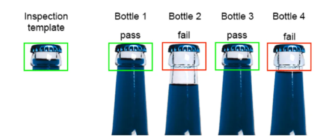
Figure 1.1: A fill-level inspection. In Bottles 2 and 4, the fill-level of the beverage inside is below a threshold and hence they fail the inspection, while bottle 1 and 3 are full and they pass.
the assembly is in frame and to trigger the camera to start inspecting different parts. The camera-based system needs to be provided with an image of the part without any inherent defects, and a proper assembly. This image is also known as the inspection template. The live image of the part on the assembly line or the image of the part to be inspected, is then compared with the inspection template to check for similarities. If the live image matches the inspection template well then it passes, else it fails and the assembly line is stopped until the part is repaired or replaced. This process is shown in figure 1.1 for a fill-level inspection system.
A fill-level inspection system has to check if the beverage in a bottle is filled up to a certain level. The first image on the left is the inspection template and the four bottles on the right are live inspections. It can be seen that bottles 1 and 3 match the inspection template well and pass, whereas, bottles 2 and 4 in which the beverage is filled less, fail.
The fill-inspection system discussed above requires just one inspection tem-plate to perform live inspections. Sometimes the part to be inspected might have some variability in its appearance and one inspection template is not enough to capture
(a) Inspection templates
(b) Parts inspected
Figure 1.2: Screws inspected in the first three images match the three inspection templates well and pass the inspection. The fourth image has a missing screw and hence the inspection fails.
this variability. The part could vary in its color or orientation and the system needs to be fed with multiple inspection templates that capture these different variations in the appearance of the part.
Figure 1.2 shows the inspection templates and live inspections for a screw inspection system. There is an inspection template provided to the system for each of the different variations in the appearances of the screw and the background frame. If one or more templates match with the part really well then the system assumes there is no defect or passes, else it signals a defect or fails.
1.2
Part appearance variability
As mentioned earlier, a camera based inspection system needs to be provided as many inspection templates as the number of distinct appearances of the parts to be inspected.
Sometimes, one of the variations in the appearance of the part to be inspected might not get considered. This might cause the system to fail, give false alarms and
(a) Inspection templates
(b) Parts inspected
Figure 1.3: The screw in the fourth image fails the inspection because there is no inspection template that matches it well. The system erroneously stops the assembly line.
erroneously stop the assembly line. As shown in figure 1.3 the system is provided with three different templates for three possible appearances. Even though the screw in the fourth live image is properly fastened, it does not match well with any of the inspection templates provided to the system, causing the system to fail.
Thus the system fails due to a particular variability in the appearance of the screw not known to it, and this is called the problem of part appearance variability. Any camera based inspection system has to be trained for this variability in part appearance to avoid such false alarms, and increase the defect detection rate.
1.3
Training for part appearance variability
To train a camera based inspection system for part appearance variability, typically, a human engineer at the factory would try to anticipate expected variations based on the different appearances of the parts. These images with different appear-ances would then be fed to the system as inspection templates. This section explains why this training process is difficult, costly and time consuming.
Figure 1.4: Variability in appearance due to change in viewing angle.
Machine parts could have a lot of variability in their appearances due to: changes in viewing angle, parts incorrectly assembled, changes in color, occlusions or changes in orientation of the parts. Each of these are explained in detail below, with an example.
Figure 1.4 shows an example where the variability in appearance is due to a change in the viewing angle of the camera. The machine might not always be in the same position when a frame is captured and the part to be inspected could be closer or further away from the camera. This change in the viewing angle leads to changes in how the part looks. It can be seen in figure 1.4 that there is variability in the appearance of the part in the live images and none of the appearances are defects.
Sometimes there is an error in the assembling that causes the part to look different. In figure 1.5 the second and third image look different because they haven’t been assembled properly. In both the images, the part has not been fastened down properly and looks loose. Thus the variability in appearance in this case is due to incorrect assembling and could be easily overlooked by a human.
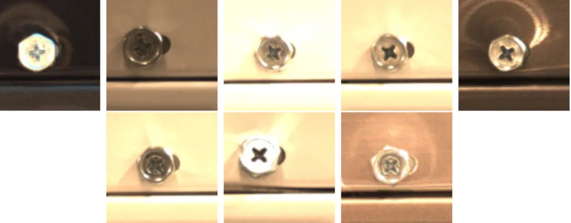
Parts and the frames on which they are fastened or attached can have different colors and specularities. Figure 1.6 shows eight different appearances of the screws. Each image has variation in the color of the frame, color of the screw and in the appearance of specularities caused due to the lighting in the factory. These colors and specularities make the parts look different and could affect the performance of
Figure 1.5: Variability in appearance due to incorrect assembling.
Figure 1.6: Variability in appearance due to change in color of background, the color of the part and specularities.
the system. It is difficult for a human to identify these different appearances and anticipate their effect on the performance of the system.
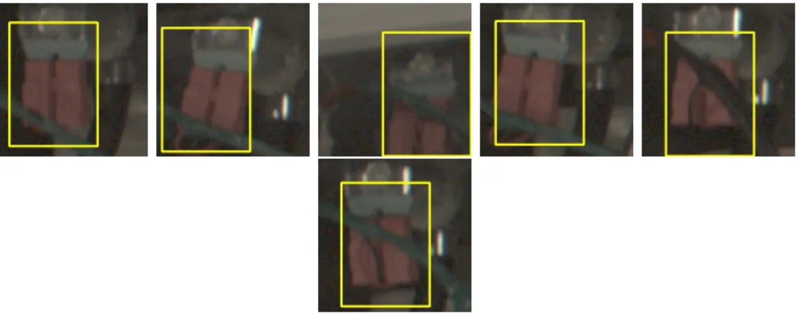
Another reason for variability in appearance could be occlusions. When some-thing obstructs or hides the view of a part, as seen from the camera, it is said that the part has been occluded or hidden or obstructed. This can cause variability in appearance as shown in figure 1.7. There is a green wire occluding the part in all the images. In one of the images the color of the wire is black and the orientation of the wire appears different in each of the seven images. The part is tilted to the right or left and is not exactly upright in most of the images. This also leads to change in appearance and it is difficult for a human to grasp these subtle changes.
Figure 1.7: Variability in appearance due to change in orientation and occlusions.
parts and sometimes they occur in combinations, which makes the problem even harder, for a human eye. In order to train the system for these complex variabilities in appearance, the human operator at the factory would have to spend a lot of time looking at tens of thousands of images of a part and find inspection templates that capture the variability in its appearance. They would have to do this for each and every part that needs to be inspected.
This is a time consuming and an error prone method and there might be a particular appearance or different appearances of a part that did not catch the eye of the human, which might cause the system to fail, as seen in figure 1.3. Some parts might have a lot of variations in their appearances and it would be really difficult for a the human eye to catch all the different cases. The system might trigger a lot of false alarms if there are not enough inspection templates that capture these variabilities in part appearance. This would stop the assembly line more frequently and reduce the throughput of the factory; thereby, making the inspection system very unreliable. Moreover, hiring human engineers for this process is a costly affair for the manufacturing company.
This thesis explains a novel approach of training a camera based inspection system to solve the problem of part appearance variability.
1.4
Background
This section gives a detailed overview of the work done by our group in the last 1.5 years to solve the problem of appearance variability or to train an inspection system for appearance variability [7]. It explains the core technologies used, the methods developed, and the inspection system prototype that was built to test these methods.
1.4.1
Template matching
Camera based inspection systems use an image processing technique called template matching for comparing the inspection templates to the live images. Tem-plate matching is a technique of finding a small part in a large image that matches a small template image. In the context of part inspections, the template image is the image of the part to be inspected, in a perfectly good condition, and, the large image is the image of a portion of the assembly where it is expected that the part would be present. In this thesis, we call the template image as the inspection template (IT) and the large image as an inspection search window or just an inspection window (IW).
As discussed earlier, in order to a inspect a part, the part inspection window is compared against all its inspection templates and depending on how well the window matches the templates, it passes and is labelled as an OK (good), or it fails and is labelled as an NOK (defect). The inspection template is slid/convolved over the entire inspection window and compared, to find out the location of the inspection template or something that looks like the inspection template, in the inspection window. A match score is generated for each point inside the inspection window. It is in the range of 0.0 to 1.0, where 0.0 indicates a total mismatch and 1.0 indicates a perfect
match. The point with the maximum score is regarded as the match location of the template inside the window. This sliding/convolving of the inspection template over the window is called template matching.
In this thesis, template matching is implemented using OpenCV, an open source computer vision and machine learning library [3]. The library provides various comparison or score generating methods for template matching. For the purpose of this thesis the normalized cross correlation (NCC) provided by the TM CCORR NORMED function is used for template matching. The algorithm produces two outputs: the best match location and the corresponding match score.
The template matching function in OpenCV is modified to generate a third output; a gray scale image called the template match image. It helps us in deciding if a particular template is appropriate for an inspection problem. This image is generated by scaling the match scores at each and every point in the inspection window to a scale from 0 to 255 where 0 is black and 255 is white and everything in between is some shade of grey. This scale is called the grey scale and the image generated using this scale is called a grey scale image. The bright spot in the image is the location with the highest score, in other words, the best match location. Ideally, there should be a single bright spot and everything else should be black or a dark shade of grey. Too many bright spots or patches indicate a poor choice of the inspection template. It indicates that too many points in the original image had a score close to the highest match score, in other words, it shows that the template is not distinct enough and is matching multiple locations in the image. Such a template would be bad for an inspection system which needs high precision and accuracy.
Figure 1.8 displays the three outputs generated by the algorithm for a partic-ular use case. In this example the template matching algorithm is used to inspect a part called hose clamp. Thus the inspection template in this case is an image of the
(a) Inspection template (b) Inspection window (c) match image
Figure 1.8: Template matching using RGB images. The hose template matches with a score of 0.85 at the best match location (center of the part) as seen in the inspection window. A bright white spot can also be seen in the template match image on the right at the same location.
hose clamp in a perfectly good condition. The IT is slid/convolved over the inspec-tion window (region where it is expected that the part is present) and a match score is generated for each and every point in the window. A blue box with dimensions equal to that of the template is drawn with its center as, the point with the highest match score, or, in other words, the best match location of the template inside the inspection window. In this case, the score at the best match location is 0.85 and a bright white spot can be seen in template match image at the same location as seen in figure 1.8c.
As mentioned earlier, the template matching algorithm has three different outputs:the match location, the match score and the match image. Sometimes, to make the process color and light independent, gradient or edge images are used instead of the original RGB images to generate these outputs [10]. Depending on the type of inspection, either or all the outputs could be generated using the original images or the gradient images of the IT and the IW like in figure 1.9.
(a) inspection template (b) inspection window (c) match Image
Figure 1.9: Template matching using edge images. The hose template matches with a score of 0.78 at the best match location (center of the part) as seen in the inspection window. A bright white spot can also be seen in the template match image on the right at the same location. The white spot in this case, is more distinct.
1.4.2
The inspection system prototype
In order to test of our methods, our group built a prototype of an inspection system. The system is capable of inspecting parts in motion and raising an alarm if a defect is detected. It can also be used to collect data (images) into a windows laptop during normal assembly operations.
1.4.2.1 Hardware
The system consists of the Basler acA2500-14gc [2], a windows laptop and LAN and power chords required for Power over Ethernet (PoE) [11]. The Basler camera has resolution of 2590x1942 pixels and captures frames at the rate of 14 frames per second. For PoE, power from a source and data from the windows laptop is transported over a CAT 6 cable via a PoE injector.
Image triggering (detect machine) Localization (find part location) Inspection (Compare, threshold and label) Figure 1.10: Overview of the inspection process.
1.4.2.2 The inspection process
The inspection process involves three stages and all three use template match-ing as their core algorithm. The first stage is detectmatch-ing if the machine is in the view of the camera. This is done by something called as image triggering. The second stage involves finding the location of the inspection windows of the parts to be inspected, also called as localization. The third stage is where the parts are inspected and the assembly line is stopped if a defect is found. Figure 1.10 gives an overview of the entire process. Each of these stages are discussed in detail in this section.
Image triggering This is the first stage in the inspection process. The unfinished assembly or the machine in an appliance manufacturing plant stops at each work station where different parts get assembled by a human or a robot. Each time it passes a work station the assembled part or parts need to be inspected. Thus the inspection system needs to be installed immediately after a work station and it needs to be notified when the machine is in view. This is done by using image triggering.
An image trigger in an image, in the context of this thesis, is that which initiates the inspection process. Just like the inspection template and the inspection window discussed earlier, we have a trigger template and a trigger search window. A trigger template is chosen such that it is present on each and every assembly on that particular assembly line. We typically select part of the background housing as shown in the red box in figure 1.11a. The trigger template is expected to be found
inside the trigger search window. The size of the search window is chosen after some trial and error; after understanding the variability in the orientation of the assembly when it is in the frame of the camera. The size of the trigger search window is set in such a way that it is not too large. A large trigger search window might slow down the image triggering process which might lead to missed inspections if the conveyor belt moves too fast.
This can be better explained using an example. Figure 1.11a shows the trigger template and a frame captured by the camera. The small image on the left is the trigger template, the blue dotted box in the image in the middle is the trigger search window, and the red box is the location of trigger where it was found with a match score of 0.72. The location of trigger in the window is indicated by the bright spot (this is the center of the red box) in the template match image, which is the rightmost image in figure 1.11a. Figure 1.11b shows where the system was setup at the factory for this use case. Basically, the machines keep moving from left to right and the live inspection system keeps searching for the trigger, in the trigger search window.
Part localization After detecting that the machine is in frame, the next step in the process of inspection is to locate the parts that need to be inspected. Assuming that all machines are assembled in a similar fashion, all parts are at fixed locations in the machine. Thus their distances from the image trigger are the same. The distances along the x axis are denoted as dx and those along the y axis are denoted as dy. Each part has a dx and dy from the trigger that is input to the system before starting the inspection process. Thus if the the location of the top left corner of the trigger inside the trigger search window is at x,y, then the top left corner of the inspection window for a part can be defined at x+dx,y+dy. The sizes of the inspection windows are pre-defined. An approach similar to the trigger search window is used for deciding the size
(a) The trigger template, the frame of the machine captured by the camera and the trigger match image. The red box shows the location of the trigger found inside the frame and the blue dotted box shows the trigger search window. A bright spot can be seen at the match location (center of the red box) in the match image.
(b) Camera installation at Samsung Electronics Home Appliances, Newberry, SC.
Figure 1.12: After locating the trigger template shown in a red box, the system locates different parts shown in green dotted boxes. The top left corner of the windows are at a fixed dx and dy from the trigger template. This is shown for the wire holder in this case.
of the inspection window. In this case, we look at the size of the inspection problem (part) and its orientation in different frames. Different parts can have inspection windows of different sizes as seen in figure 1.12. Figure 1.12 shows the machine with different parts. The blue dotted boxes are the inspection windows of different parts that need to be inspected for defects. The dx and dy for the part called wire holder is shown in the figure. Both, dx and dy have negative values in this case because the part is on the left and above the image trigger.
Part Inspection Once the machine is frame and the system knows the probable locations of different parts, it is time to inspect. Inspection templates for each part are fed to the system before starting the inspection process. Each part can have varying number of inspection templates. The inspection templates for a part are compared
with the respective inspection window using template matching and a template match score and a match image is generated for each template. If the template that matches the best, (has the highest match score and the brightest spot in its match image) has a match score lower than a threshold (for that part) then it is assumed that there is a defect and the part is labelled as an NOK and an alarm is raised, else it is an OK. As shown in figure 1.13, after locating the inspection window of the white water valve using part localization, the templates of the white water valve are compared with the window using template matching. The template with the highest score of 0.85 is shown on the left and its match image with the best match location indicated by a bright spot is shown on the right of the machine. The match location is shown in the machine with a red box with size equal to the size of the template. The score of 0.85 is greater than a threshold and hence it is assumed that the part is OK or has no defects. This method is implemented for all the parts shown in figure 1.12 simultaneously as soon as the machine is in frame.
Figure 1.13: A frame of the machine with different parts. After locating the image trigger, the system has defined an inspection window for the white water valve at a fixed distance from the image trigger. A match score is generated for the part (white water valve) inside the inspection window. The match score (0.85) is higher than a threshold and is hence labelled as an OK. The template match image of the inspection template and the window is also shown.
Image triggering (locate the trigger in the stored frame) Localization (locate the IWs) Crop (crop and store)
Figure 1.14: Overview of the cropping process.
1.4.3
The data collection process
Data is collected to test, and further develop our methods of training the inspection system for appearance variability. The data collection process developed by our group is similar to the inspection process and is performed during normal assembly operations. Once the machine is in frame, as detected by the image trigger, instead of localizing and inspecting different parts, the frame is stored in a database (windows laptop).
1.4.4
The cropping process
After the data has been collected, we need images of the inspection windows of the different parts to be inspected. For this reason, a cropping program which crops out inspection windows from all the frames (data) collected in the data collection process, was developed by our group.
This process is again, similar to the inspection process. As the inspection windows of parts are defined with respect to the location of the trigger in the image, image triggering is performed in order to find the location of the trigger. Next the location of the top left corner of the inspection windows of different parts are found out and the parts are cropped. Figure 1.14 gives an overview of this process.
1.4.5
Clustering to find appearance variability
As discussed earlier, it is a time consuming task and an error prone task for a human to go through each and every inspection window and find out the differ-ent variations in the appearance of each and every inspection problem. In order to solve this problem a method to automatically learn part appearance variability was developed by our group at Clemson [7].
It is based on an unsupervised machine learning algorithm known as clustering and automatically learns the variability in appearance of the parts to be inspected. It takes in as input, all the inspection windows generated by the cropping program, an inspection template of the part to be inspected and a configuration file. It then forms different clusters or groups of IWs that have similar part appearances. Each cluster has a seed which represents the variability in the appearance captured by that particular cluster; in other words, all parts in that cluster look more or less the same in comparison to the seed.
Now, instead of looking at each and every image, the human engineer can just look at the seeds and pick the ones that vary in appearance and are not defects. The method is generic and not problem specific and automatically suggests inspection templates that capture the variability in appearance of parts to be inspected; it does not require any human interference once given the required inputs.
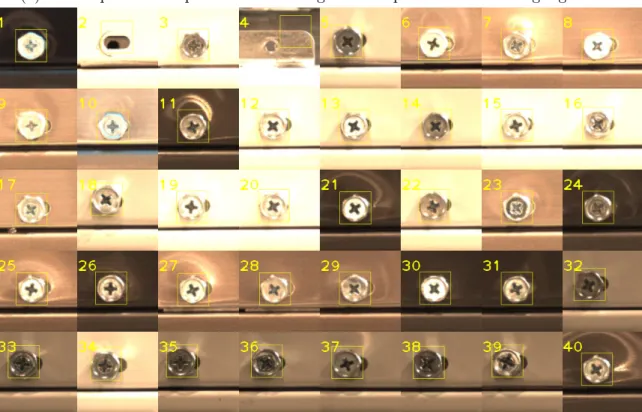
Figure 1.15 shows the output of the clustering algorithm for the screw use case. It takes in as input the inspection template as shown in figure 1.15a, and approximately 3,000 inspection windows of the screw. Different variations in the appearances of the screw can be seen in figure 1.15 as found by the algorithm. Inside each of the windows there is a bounding box that highlights part. The size of these highlights is same as the size of the input template, as shown in figure 1.15a. These
(a) The inspection template of the screw given as input to the clustering algorithm.
(b) A collage of the 40 cluster seeds of the screw generated by the clustering algorithm.
Figure 1.15: The 40 cluster seeds capture different variations in the appearance of the screw including defects.
are called seed templates or seeds. These seed templates of all the clusters can be suggested to a human engineer as probable inspection templates which could be used for live inspections as seen in figure.
1.4.5.1 The clustering algorithm
This section reviews the clustering method described in [7]. The system is based on a variant of the k-means clustering algorithm. The k-means clustering algorithm divides a large dataset into k groups because there are k seeds or k points within the data set that are manually chosen with some heuristics. The algorithm has two steps: assignment and update. In the assignment step, each data point is assigned to one of k seeds. Each data point is assigned to the seed which is the closest to it, in terms of a distance metric. At the end of this step we have k groups with their respective k seeds, where the seed of a group is one of the points in the group that represents the group. In the update step these k seeds are updated so as to better represent their group. Next, the algorithm goes back to the assignment step and this loop of assignment to update to assignment goes on until a stopping condition is met. At the end, k distinct groups of points are formed, where each group has a distinct feature. In the case of clustering inspection windows of a part, the k seeds would represent the k distinct appearances of the part.
The algorithm developed by our group takes in as input all the inspection windows of a part, an inspection template and a threshold that defines the stopping condition. Unlike k-means clustering where the user provides k different seeds, the algorithm has to be given only one seed which is the template (one ideal appearance of the part) of the part to be inspected.
At the beginning, in the assignment step, all images are assigned to one clus-ter. A match score and a match location is generated for all the inspection windows
after comparing them with the seed using template matching, and the variance of all the match scores is calculated. This is the first cluster or group of images formed by the algorithm. In the update step, the least scoring member of this cluster (part which looks very dissimilar to the seed) is assigned as the second seed. Now, the scores and locations are calculated with respect to both the seeds for all the inspec-tion windows by using template matching. Next, in the assignment step, cluster membership is assigned to a window according to the seed which has a better match score for that particular window. At the end of this step, we have two clusters with their two respective seeds. Now, the variances of scores for cluster one and for cluster two are calculated. In the update step, the least scoring member of the cluster with the maximum score variance (cluster which has a lot of variability in the appearance of its members) is assigned as the the third seed. Now, the scores and locations are calculated with respect to three seeds for all the inspection windows. This loop goes on until the cluster with the maximum variance is below a certain threshold called the maximum cluster variability threshold or MCVT. At the end, the algorithm gen-erates k different groups of inspection windows with their match locations and match scores with respect to their respective k seeds. Each seed represents the variability in appearance of the part captured by its group or cluster. Information about each cluster such as the seed, number of members, score variance, match locations and scores of each member are stored in a text file.
Unlike k-means clustering the value of k is not pre-defined. It depends on the MCVT, which in turn, depends on the complexity of the inspection problem and is calculated using normalized difference accumulated image (NDAI) of the part to be inspected. The entire algorithm, along with the tuning of MCVT using the NDAI, is discussed in more detail in [7].
1.5
Related Work
W. A. Perkins developed a system that could classify different parts and detect defects at the same time. There were two parts to the inspection system, one was de-termining inspection regions of a part and then dede-termining test parameters for those regions in order to inspect the part [5]. C. Tsatsoulis and King-sun Fu developed a programming language named SAIL (simple assembly inspection language) for visual inspection of assemblies. The system is based on measurement of different charac-teristics of parts. It is described in [8]. Progress in the field of machine vision and an overview of the real-world applications can be found in [4]. It describes popular software and hardware tools required to build a machine vision system. Different im-age registration methods are discussed in [13]. The most recent work which is closely related to what we have done is a patent by Cognex Corporation [6].
All the above works are part specific, whereas, we are trying to solve the problem using a generic approach which can be applied to any inspection problem. We also consider the problem of a human engineer at a manufacturing plant being able to use our methods.
1.6
Novelty
The novelty of this thesis lies in three components of the inspection system:
• Training the inspection system for appearance variability: Previous work developed a tool (clustering) that could learn part appearance variability [7]. We performed a set of experiments, trying different ways of using the tool to train an inspection system. Variations included how long to run the clustering, how to select inspection templates from its output, whether or not
to use NOK templates in addition to OK templates, and when and how to tweak the inspection settings (pre-processing, IW size, IT size). The goal was to maximize the defect detection rate while minimizing the false alarms. Lessons learned from performing these tests on 9 different inspection problems were used to build a decision tree that could be used by engineers for training the inspection system on future inspection problems. We also report our inspection accuracies and the training process for all the 9 inspection problems.
• Data collection: Previous work collected 1,052 images for 3 inspection prob-lems. In this work we collected a large amount of new data: 39,268 frames for 6 inspection problems (EMI filter, red water valve, white water valve, hose clamp, wire holder and the pressure sensor), 23,247 frames for 2 more inspec-tion problems (thermistor, screw near thermistor) and 3,987 frames for another inspection problem (back screw). A total of 249,371 images were collected for 9 inspection problems.
• The clustering algorithm: The clustering algorithm developed previously [7] was modified to allow it to run on arbitrary sized data sets. This was needed because the data we collected was orders of magnitude larger than in previous work.
Chapter 2
Methods
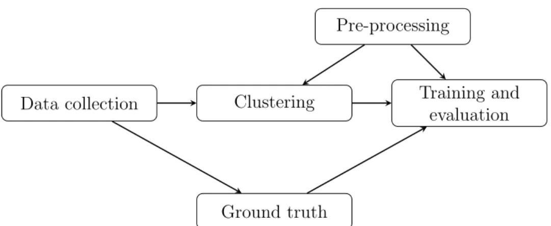
Figure 2.1 overviews the methods used for our experiments in order to train an inspection system prototype for part appearance variability. After collecting data, parts to be inspected are cropped and manually reviewed for defects (ground truth). The clustering algorithm is run on the crops of the parts to be inspected. The clustering algorithm outputs all the cluster seeds or the different appearances of the parts. The cluster seeds are then used as training templates to train and evaluate an inspection system prototype by comparing its results with the manually reviewed data. Different pre-processing and training options are tested to improve the results our methods with a goal of reducing false alarms and increasing the number of defects detected. Each of these processes are discussed in detail in this chapter.
2.1
Data collection
We collected data on three different occasions. The first data collection oc-curred over a period of 3 months as we tested different variations of pre-processing and camera settings. The second data collection occurred at another assembly line
Data collection Clustering Training and evaluation Pre-processing
Ground truth
Figure 2.1: Overview of the methods used for our experiments.
location for 2 new parts. The third data collection used cameras already installed at SEHA and being used by their existing Q-eye inspection system. All the data collected has been summarized in table 2.1.
2.1.1
The low gain data set
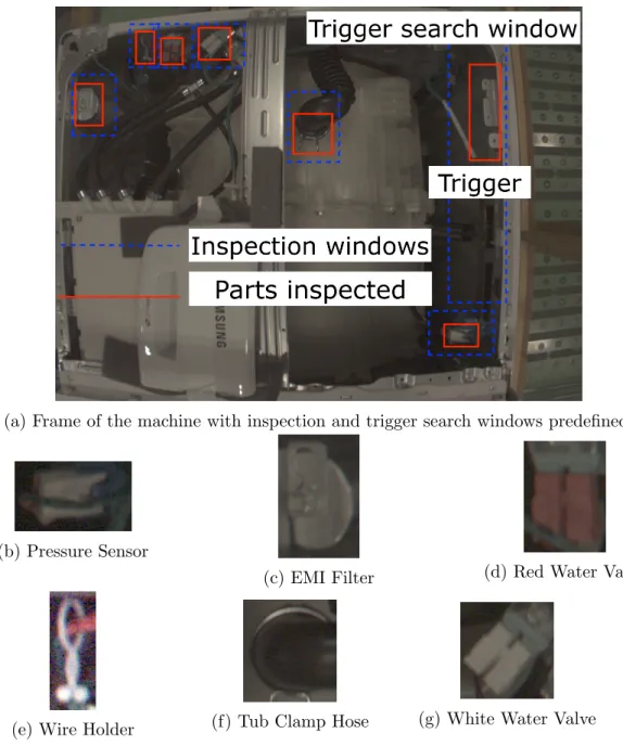
This data set contains parts from the frame shown in figure 2.2. A total of 39,268 frames were collected, 2 frames per machine. Out of the 12 parts in the frame that needed inspection, we chose only 6 to do our experiments on due to occlusions or poor lighting conditions. This section describes each of the 6 parts and what they were inspected for, viz., the white water valve, the red water valve, the pressure sensor, the tub clamp hose, the EMI filter and the wire holder. Each of these can be seen in figure 2.2.
White water valve Valves in a washing machine are mechanical devices that con-trol the amount of flow of hot and cold water inside the washer. They are connected to water hoses that transports the water inside the washer. The valves have ports which
Data-set No. of Machines Start date End date Notes
Pilot 3,347 12/6/2018 12/10/2018 First collection
test.
Low Gain 19,634 1/11/2019 1/29/2019 Largest dataset.
After collection, it was determined that the camera gain
was too low (dark images).
(figure 2.2)
High Gain 3,378 2/11/2019 2/12/2019 Adjusted gain
and exposure time to increase
image brightness.
New Model 4,520 2/12/2019 2/21/2019 New washing
machine model. Production slow
(about 1 machine/10
minutes).
Thermistor 11,625 9/26/2019 10/10/2019 Most recent
data collection to demo our system to the Samsung executives. (figure 2.9)
SEHA 3,987 03/09/2019 03/11/2019 This is the data
provided by SEHA (figure
2.12) Table 2.1: Data collection summary.
(a) Frame of the machine with inspection and trigger search windows predefined.
(b) Pressure Sensor
(c) EMI Filter (d) Red Water Valve
(e) Wire Holder (f) Tub Clamp Hose (g) White Water Valve
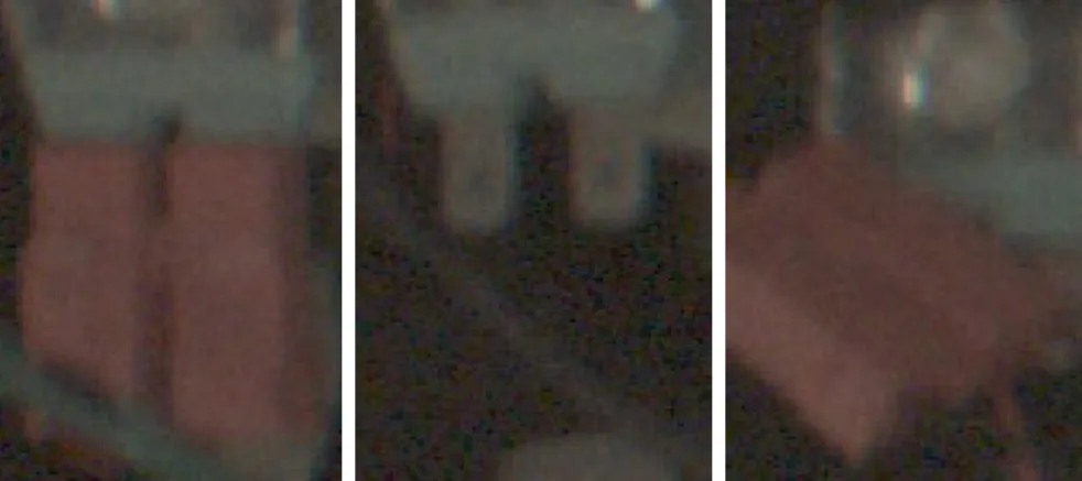
Figure 2.3: In the first figure, the white valve is present and fully secured and con-nected to the green mount (OK). Next, it is is absent (NOK). In the third figure, it is dangling (NOK).
are used to send electric power to the valve to open and close the flow of water based on the user defined settings of temperature and volume. These ports have solenoid valves which carry electric current. Incorrect assembling of the solenoid valves might lead to the tub not getting filled properly or the temperature of the water not being as defined by the user.
The white valve is inspected to make sure it is present and connected to the green mount as shown in figure 2.3. In this thesis we focus on detecting presence or absence of the valve. We do not try to find whether the valve is partially or fully connected, we are just inspecting to make sure it is connected and not dangling or totally absent.
Red water Valve The red water valve is similar to the white water valve, but red in color. It is also inspected to make sure it is present and fully secured and connected to the green mount and not dangling or absent, as shown in figure 2.4.
Tub Clamp Hose A hose is a tube that transports liquids from one location to other. In this case, it is the hose that provides water to the tub of the machine. The hose clamps are used to attach the hose to the tub via a fitting such as a barb. The hose is inspected to check whether it is fully seated on the tub and that the clamp is
Figure 2.4: In the first figure, the red valve is present and fully secured and connected to the green mount (OK). Next it is absent (NOK). In the third figure, it is dangling (NOK).
Figure 2.5: In the first figure, the hose is seated on the tub and the clamp is secure (OK). Next, it is occluded by an object and it cannot be inspected (NOK).
all the way secure as shown in figure 2.5 (to avoid water leakage).
EMI Filter The EMI (Electromagnetic interference) filter is a device that reduce the high frequency (radio frequency) noises present on the power lines that can de-grade the performance of the electronic equipment inside the machine. It is inspected to make sure it is completely fastened down and is not loose as shown in figure 2.6.
Figure 2.6: In the first figure, the EMI filter is completely fastened down (OK). Next, it is not fastened down completely (NOK).
Figure 2.7: In the first figure, the white connector of the pressure sensor is snapped in completely inside the blue mount (OK). Next, the part is occluded or it is a trigger failure (NOK).
needed for different cleaning cycles. The pressure sensing module is inspected to make sure it is snapped in completely to its mount as shown in figure 2.7.
Wire Holder The wire holder is designed to hold all the wire harnesses and avoid any dangling wires inside the machine. A wire harness is a group of wires that transmit power and other signals. It is important to manage the wiring so that wires are not left dangling around. Dangling wires have a risk of breaking or getting shorted and that might affect the performance of the washing machine, or it might just stop working due to no power.
Figure 2.8: In the first figure, the wire harness is inside the wire holder (OK). Next, the wire holder is not tied and the wire is left dangling outside of the holder (NOK). Next, the holder is not tied and the wire can slip out (NOK). In the fourth figure, the wire is not going through the holder and in the last figure the holder is absent (NOKs).
holder and the holder is completely snapped into the frame of the machine. It is also inspected to make sure that it has a knot, so as to not allow the wire harness to slip out of the holder.
2.1.2
The thermistor data set
This data was collected to demo our system to the Samsung executives. We collected a total of 23,247 frames of machines, approximately 2 frames per machine.
Figure 2.9: Thermistor data set: A frame of the tub of the machine; Two different parts inspected in 23,247 such frames.
the thermistor as shown in figure 2.9.
Thermistor screws A thermistor is a resistor, the resistance value of which, changes based on the temperature of the surroundings. Thus it acts as a temperature sen-sor. It is inserted inside the tub (where the clothes get washed) to measure the temperature of the water.
The thermistor is attached to a frame with 2 screws. The thermistor is inserted into the tub and and the two screws are tightened to hold it in place inside the tub. Loose screws can cause water leakage, damaging other electrical components of the machine. Thus they are inspected to make sure the silver frame is fully seated and screwed into the tub as shown in figure 2.10.
Screw near thermistor The screw near the thermistor helps with some of the electrical connections. It is inspected to make sure it is present and screwed tightly
Figure 2.10: In the first figure, the thermistor frame is screwed into the tub completely (OK). In the second figure, there is a human hand covering the part and we cannot inspect it (NOK).
Figure 2.11: In the first figure, the screw is screwed tightly on to the frame (OK). In the second figure, the screw is absent (NOK).
into the silver frame as shown in figure 2.11
2.1.3
The SEHA data set
The SEHA data set was provided to us by the Samsung Electronics Home Appliances (SEHA) factory and contains 3987 frames of the screws on the back of the machine, on the left and right side as shown in figure 2.12. Out of the 7 screws, the one on the top left side and next to the grey colored frame (right side of the frame) was used for our experiments.
Top left screw on the back The top left screw was inspected to make sure it is tight and screwed completely into the frame as shown in figure 2.13.
(a) Top Left Screws
(b) Top Right Screws
Figure 2.12: Data Collection 3: Top left and top right corners of the back of the machine; Four screws at the top left corner and three screws at the top right corner inspected.
Figure 2.13: Screws on the back of the washing machine. The first figure is an OK screw. Next, the screw is absent (NOK). In the last figure, the screw is not screwed into the frame (NOK).
Training for appearance
variability
Inspection template size Template match method
Image pre-processing method Inspection window size
Figure 2.14: Different pre-processing options developed to improve the results of the clustering algorithm and other methods.
2.2
Pre-processing
Figure 2.14 shows the several pre-processing options we developed, while trying to improve the results of our methods. Some helped clarify part appearances, while others improved part comparisons. Image pre-processing methods like histogram equalization and median blurring were used to improve contrast and remove noises in the images. Different template match methods like RGB or Edge matching were tried, to improve part comparisons while clustering. Other options developed were changing the inspection template size and the inspection window sizes, in order to improve the localization of the areas of inspection. Each of these pre-processing options are discussed in this section.
2.2.1
Inspection window size
Sometimes the part to be inspected is not centered or partially visible or clipped inside the inspection window. To solve this problem, the size of the inspection window is increased and all the inspection windows are re-cropped. The inspection windows are cropped in such a way that there are no nearby parts or other similar
(a) Inspection search window too small as part is not fully visible or clipped and the local-ization is poor.
(b) New inspection window with an increased size leads to better localization.
Figure 2.15: The system has an option to adjust the window size if the part is not fully visible in the cropped images.
objects in view. An example is shown in figure 2.15.
The inspection window for the white water valve was cropped originally small as shown in figure 2.15a. For a couple of thousand images the valve was at the right bottom and some part of the green mount was out of the frame. To solve this problem the size of the window was increased and all the inspection windows were re-cropped. Now, the templates were able to latch on to the correct location as shown in figure 2.15b.
2.2.2
Size of the inspection template
In our experiments, we consider the following factors while deciding the size of the template:
Area of inspection The size of the inspection template is chosen such that it covers the entire area of inspection, at minimum. Many times, the size of the template is increased to include any nearby context that might act as a cue for defects or might
help the template matching algorithm to locate the area of inspection easily (have a good template match image).
Appearance of defects Defects are looked at to get a better understanding of the differences between defects and OK parts. This information is used to adjust the size of the template so that it is able to capture defects and not just OK parts.
Variation in size All the cropped parts are checked for variations in the size of the area of inspection. Sometimes a part appears larger due to a change in camera angle or change in orientation of the assembly, other times, a part could have variable sizes, both cases need to be considered.
Image gradients Another important factor to consider is the image gradients. The image gradients are looked at and analyzed for defect and OK images. Sometimes they act as cues for defects, other times they help in the process of localization (edges of the nearby context).
2.2.3
Image pre-processing method
For the clustering to work, it important for the part to be clearly visible inside the inspection widows. Image processing techniques like histogram equalization and median blurring are used to solve this problem. Histogram equalization improves contrast and median blurring removes the noises in the image. This can be seen in figure 2.16 for the white water valve use case.
That being said, it is not always necessary to use image pre-processing. Some-times the lighting conditions are good and the image pre-processing only hurts, if not improves the performance. Important edge information in the area of inspection
(a) Inspection window of an OK white water valve and its edge image before and after image pre-processing.
(b) Inspection window of an NOK white water valve and its edge image before and after image pre-processing.
Figure 2.16: Pre-processing drastically improves the edges of the parts which are dimly lit.
Figure 2.17: Pre-processing fails for this use case because the lighting is good and pre-processing is not required.
could be lost if pre-processing is used when not required, as shown in figure 2.17. Table 2.2 gives information whether the image pre-processing option was ac-tivated or not, for all the 9 use cases. In our data sets, the screws were well lit and had strong edges, and hence, did not require image pre-processing to be done.
Inspection problem
Image pre-processing White
water valve Yes
Red water
valve Yes
Tub clamp
hose Yes
EMI Filter Yes
Pressure
sensor Yes
Wire holder Yes
Thermistor
screws Yes
Screw near
thermistor No
Back screw No
Table 2.2: Image pre-processing usage for different use cases depending on the strength of edges and lighting conditions.
2.2.4
Template matching method
The template matching algorithm has two different outputs, one is the match location and the other is the match score. These outputs could be generated using edge images or RGB images of the IT and IW, depending on the inspection problem.
Finding the match location Three factors are considered when deciding on the matching technique to be used for finding the match location: Distinctiveness of the edges in the area of inspection with respect to the nearby context, distinctiveness of the color of the area of inspection with respect to nearby context, color variation in the area of inspection and the nearby context and occlusions. The table 2.3 gives information regarding the matching technique used in each of the 9 use cases and why it was used.
Inspection problem
Match
method Notes
White
water valve Either
Part has distinct color and edges and no occlusions. Both RGB and edge matching work well. Red water
valve RGB
Part has distinct color and edges but a lot of occlusions. Hence RGB matching (occlusions mess
up edges) Tub clamp
hose RGB
Edges of the area of inspection are weak and there are occlusions. Part has a distinct
color. EMI Filter Either
Part has distinct color and edges. Both RGB and edge
matching work well. Pressure
sensor RGB
Part has distinct color and edges but a lot of occlusions. Hence
RGB match.
Wire holder Either Part has distinct color and edges. Both work same. Thermistor
screws RGB
Part has distinct color and edges but has occlusions. Hence RGB
match. Screw near
thermistor Edge
Part has a distinct circular edge. Hence edge match.
Back screw Edge
Part has distinct color and edges and no occlusions. But there are
too many color variations.
Finding the match score For the parts inspected in this thesis, matching edge images of the ITs and the area of the inspection generate a wide range of scores and it is easy to decide on a threshold (score), below which, all the parts are labelled as defects. This is because the edges in an NOK or an image of a defective part are very different from those in an OK image.
Matching RGB images generate scores in a very narrow range and it is really difficult to decide on a threshold on such a narrow range of scores. Hence RGB matching is not used to score any of the inspection problems discussed in this thesis.
2.3
Ground truth
Once the inspection windows are cropped, they are manually reviewed or ground truth for defects. This helps us in understanding the appearance of the defects, and also helps us in evaluating the performance of the system in detecting defects, after the training process is completed.
The cropping process crops all the inspection windows of a part into one folder. These are then viewed using the icon view option of the macOS Finder (file explorer) as shown in figure 2.18. In the icon view option, one can see many inspection windows at a glance and that speeds up the reviewing process. As shown in the figure, 28 inspection windows of the white water valve were reviewed or ground truth at a time. It took on an average of 180 minutes to ground truth a data set of approximately 39,000 inspection windows for one use case.
Table 2.4 gives information regarding the number of images cropped and the number of defects found for all the 9 use cases. A total of 249,371 images were
Figure 2.18: Process of manual reviewing for defects.
cropped for 9 inspection problems and there were 2 to 180 defects per inspection problem. Some of the images failed to crop due to trigger failures (failed image triggering) or out of bound inspections (part not in frame).
2.4
Clustering
For this thesis, the clustering algorithm is modified to process a much larger amount of data. The method now has very less memory requirements and can run on arbitrary sized data faster.
The implementation in [7] loads all the inspection windows of the part from the database in order to run clustering. The size of an inspection window can be of
Inspection problem No. of frames Frames analyzed Fail to
crop Defects Defect rate
White water valve 39,268 32,242 1,602 83 0.26 % Red water valve 39,268 38,447 821 89 0.23 % Tub clamp hose 39,268 39,268 0 17 0.04 % EMI Filter 39,268 39,268 0 31 0.08% Pressure Sensor 39,268 13,009 26,259 2 0.02 % Wire holder 39,268 36,658 2,610 180 0.49 % Thermistor screws 23,247 23,247 0 12 0.05 % Screw near thermistor 23,247 23,245 2 23 0.1 % Back screw 3,987 3,987 0 39 1.0 %
Table 2.4: Crops and ground truths for all the use cases.
several megabites and thus the program might require several gigabytes of memory to run. If we have hundreds of thousands of images then the memory requirement can go up to several terabites. Considering the time complexity of the clustering algorithm of O(N2), that means more memory usage and more time to run. In contrast, the implementation in this thesis requires very less memory and runs faster for large data sets. At any given point during which the program runs, there are only two images that are loaded. Thus the memory requirement to run the program is only a few megabytes. This updated version can now handle arbitrary sized data unlike the previous implementation, where if the data size was greater than the available memory, the program would crash because it couldn’t load all the images.