A Novel Hyperbolic Smoothing Algorithm for Clustering Large Data Sets

A Novel Hyperbolic Smoothing Algorithm for

Clustering Large Data Sets

Adilson Elias Xavier Vinicius Layter Xavier

Dept. of Systems Engineering and Computer Science Graduate School of Engineering (COPPE)

Federal University of Rio de Janeiro P.O. Box 68511

Rio de Janeiro,RJ 21941-972, BRAZIL e-mail: {adilson,vinicius}@cos.ufrj.br

Abstract

The minimum sum-of-squares clustering problem is considered. The math-ematical modeling of this problem leads to a min−sum−min formula-tion which, in addiformula-tion to its intrinsic bi-level nature, has the significant characteristic of being strongly nondifferentiable. To overcome these difficul-ties, the proposed resolution method, called Hyperbolic Smoothing, adopts a smoothing strategy using a special C∞ _{differentiable class function. The} fi-nal solution is obtained by solving a sequence of low dimension differentiable unconstrained optimization This paper presents an extended method based upon the partition of the set of observations in two non overlapping parts. This last approach engenders a drastic simplification of the computational tasks.

Keywords: Cluster Analysis, Pattern Recognition, Min-Sum-Min Problems, Nondifferentiable Programming, Smoothing

1

Introduction

Cluster analysis deals with the problems of classification of a set of pat-terns or observations, in general represented as points in a multidimensional space, into clusters, following two basic and simultaneous objectives: patterns in the same clusters must be similar to another (homogeneity objective) and different from patterns of other clusters (separation objective), see Hartingan (1973) and Sp¨ath (1980).

A particular clustering problem formulation is considered. Among many criteria used in cluster analysis, the most natural, intuitive and frequently adopted criterion is the minimum sum-of-squares clustering (MSSC). It is a criterion for both the homogeneity and the separation objectives.

The minimum sum-of-squares clustering (MSSC) formulation produces a mathematical problem of global optimization. It is both a nondifferen-tiable and a nonconvex mathematical problem, with a large number of local minimizers.

In the cluster analysis scope, algorithms use, traditionally, two main strategies: hierarchical clustering methods and partition clustering methods (Hansen and Jaumard (1997) and Jain et alli (1999)). This paper adopts a different strategy, a smooth approach, which was originally presented in Sousa(2005) and Xavier(2008).

For the sake of completeness, we present first the smoothing of the min−

sum−min problem engendered by the modeling of the clustering problem. In a sense, the process whereby this is achieved is an extension of a smoothing scheme, called Hyperbolic Smoothing. This technique was developed through an adaptation of the hyperbolic penalty method originally introduced by Xavier (1982). By smoothing, we fundamentally mean the substitution of an intrinsically nondifferentiable two-level problem by a C∞ _{unconstrained} differentiable single-level alternative.

Additionally, the paper presents a extended faster procedure. The basic idea is the partition of the set of observations in two non overlapping parts. By using a conceptual presentation, the first set corresponds to the obser-vation points relatively close to two or more centroids. This set of observa-tions, named boundary band points, can be managed by using the previously presented smoothing approach. The second set corresponds to observation points significantly closer to a single centroid in comparison with others. The set of observations, named gravitational points, is managed in a direct and simple way, offering much faster performance.

For the purpose of illustrating both the reliability and the efficiency of the method, a set of computational experiments was performed, making use of traditional test problems described in the literature.

2

The Clustering Problem Transformation

Let S ={s1, . . . , sm} denote a set of m patterns or observations from an Euclidean n-space, to be clustered into a given number q of disjoint clusters. To formulate the original clustering problem as a min−sum−min

problem, we proceed as follows. Let xi, i= 1, . . . , q be the centroids of the clusters, where each xi ∈ Rn. The set of these centroid coordinates will be represented by X ∈Rnq_{. Given a point s}

j of S, we initially calculate the distance from sj to the center in X that is nearest. This is given by

zj = minxi∈X ksj −xik2.

The most frequent measurement of the quality of a clustering associated to a specific position of q centroids is provided by the sum of the squares of these distances, which determines the following problem:

minimize m X j=1 z2 j (1) subject to zj = min i=1,...,q ksj −xik2, j = 1, . . . , m.

Considering its definition, each zj must necessarily satisfy the following set of inequalities: zj − ksj −xik2 ≤0, i = 1, . . . , q. Substituting these

inequalities for the equality constraints of problem (1), a relaxed problem would be obtained.

Since the variables zj are not bounded from below, the optimum solution of the relaxed problem will be zj = 0, j = 1, . . . , m. In order to obtain a bounded formulation, we do so by first letting ϕ(y) denote max{0, y} and then observing that, from the set of constraints in (1), it follows that

q X

i=1

ϕ(zj − ksj−xik2 ) = 0, j = 1, . . . , m. (2)

By using (2) in place of the set of constraints in (1) and by including a perturbation ² >0 we would obtain the bounded problem:

minimize m X j=1 z2 j (3) subject to q X i=1 ϕ(zj − ksj−xik2 ) ≥ ε , j = 1, . . . , m.

Since the feasible set of problem (1) is the limit of that of (3) when

²→0+, we can then consider solving (1) by solving a sequence of problems

Analyzing the problem (3), the definition of function ϕ endows it with an extremely rigid nondifferentiable structure, which makes its computational solution very hard. From this perspective, for y ∈ R and τ > 0, let us define the function:

φ(y, τ) = ³

y+py2_+τ2

´

/2. (4)

Function φ constitutes an approximation of function ϕ. To obtain a completely differentiable problem, it is yet necessary to smooth the Euclidean distance ksj−xik2. For this purpose, let us use the function

θ(sj, xi, γ) = v u u tXn l=1 (sl j −xli)2 + γ2 (5)

By using function θ in place of the distance ksj −xik2, it is obtained

the completely differentiable problem:

minimize m X j=1 z2_j (6) subject to q X i=1 φ(zj −θ(sj, xi, γ), τ)≥ε, j = 1, . . . , m.

So, the properties of functions φ and θ allow us to seek a solution to problem (3) by solving a sequence of subproblems like problem (6), produced by the decreasing of the parameters γ →0 , τ →0, and ε→0.

On the other hand, given any set of centroids xi, i = 1, . . . , q, due to the increasing convex property of the hyperbolic smoothing function φ,

the constraints of problem (6) will certainly be active. So, it will at last be equivalent to problem: minimize m X j=1 z2 j (7) subject to hj(zj, x) = q X i=1 φ(zj−θ(sj, xi, γ), τ) − ε = 0, j = 1, . . . , m. The dimension of variable domain space of problem (7) is (nq +m).

However, it has a separable structure, because each variable zj appears only in one equality constraint. Therefore, as the partial derivative of h(zj, x) with respect to zj, j = 1, . . . , m is not equal to zero, it is possible to use the

Implicit Function Theorem to calculate each component zj, j = 1, . . . , m as a function of the centroid variables xi, i = 1, . . . , q. In this way, the unconstrained problem minimize f(x) = m X j=1 zj(x)2 (8)

is obtained, where each zj(x) results from the calculation of the unique zero of each equation hj(zj, x) = q X i=1 φ(zj−θ(sj, xi, γ), τ) − ε = 0, j = 1, . . . , m. (9)

Again, due to the Implicit Function Theorem, the functions zj(x) have all derivatives with respect to the variables xi, i= 1, . . . , q, and therefore it is possible to calculate the gradient of the objective function of problem (8),

∇f(x) = m X j=1 2zj(x)∇zj(x), (10) where ∇zj(x) = − ∇hj(zj, x) / ∂ hj(zj, x) ∂ zj , (11)

while ∇hj(zj, x) and ∂ hj(zj, x)/∂ zj are obtained from equations (4), (5) and (9).

In this way, it is easy to solve problem (8) by making use of any method based on first order derivative information. At last, it must be emphasized that problem (8) is defined on a (nq)−dimensional space, so it is a small problem, since the number of clusters, q, is, in general, very small for real applications.

3

The Partition Procedure

The calculation of the objective function of the problem (8) demands the determination of the zeros of m equations (9), one equation for each obser-vation point. Now, it will be presented a faster procedure. The basic idea is the partition of the set of observations in two non overlapping parts. By using a conceptual presentation, the first set corresponds to the observation points that are relatively close to two or more centroids. The second set corresponds to the observation points that are significantly close to a unique centroid in comparison with the other ones.

So, the first part JB is the set of boundary observations and the second is the set JG of gravitational observations. Considering this partition, equation (8) can be expressed as a sum of two independent components.

minimize f(x) = m X j=1 zj(x)2 = X j∈JB zj(x)2 + X j∈JG zj(x)2. (12) minimize f(x) = f1(x) +f2(x). (13)

The first part of expression (13), associated with the boundary observa-tions, can be calculated by using the previous presented smoothing approach, see (8) and (9). The second part of expression (13) can be calculated by using a faster procedure, as we will show right away. Let us define the two parts in a more rigorous form. Let be xi, i= 1, . . . , q be a referential position of centroids of the clusters taken in the iterative process.

The boundary concept in relation to the referential point x can be easily specified by defining a δ band zone between neighboring centroids. For a generic observation s ∈ Rn_{, we define the first and second nearest} distances from s to the centroids: d1(s, x) = ks−xi1k = miniks−xik

and d2(s, x) = ks−xi2k = mini=6 i1ks−xik , where i1 and i2 are the

labeling indices of these two nearest centroids. By using the above definitions, let us define precisely the δ boundary band zone:

Zδ(x) = {s ∈Rn |d2(s, x) − d1(s, x) < δ} (14)

and the gravitational region, this is the complementary space:

Gδ(x) = {s∈Rn − Zδ(x)}. (15) Figure 1 illustrates in R2 _{the Z}

δ(x) and Gδ(x) partitions. The central lines form the Voronoy polygon associated with the referential cen-troids xi, i = 1, . . . , q. The region between two parallel lines to Voronoy lines constitutes the boundary band zone Zδ(x).

Now, the two sets can be defined in a precise form: JB(x) ={j|sj ∈Zδ(x)} and JG(x) = {j|sj ∈Gδ(x)}.

Proposition 1: Let s be a generic point belonging to the gravitational region Gδ(x), with nearest centroid i1. Let x be the current position of

the centroids. Let ∆x = maxikxi − xik be the maximum displacement of the centroids. If ∆x < δ then s will continue to be nearest to centroid

xi1 than to any other.

Since δ ≥ ∆x, Proposition 1 makes it possible to calculate exactly expression (12) in a very fast way. First, let us define the subsets of gravita-tional observations associated with each referential centroid:

Ji(x) = ½ j ∈JG| min l=1,...,qksj −xlk = ksj −xik ¾ (16)

Figure 1: The Zδ(x) and Gδ(x) partitions.

The gravity centers of the observations in each non-empty subset are given by vi = 1 |Ji| X sj∈Ji sj, ∀i= 1, . . . , q. (17) Let us consider the second sum in expression (12). It will be computed by taking into account the gravity centers defined above.

minimize f2(x) = X j∈JG zj(x)2 = q X i=1 X j∈Ji ksj−xik2 = q X i=1 X j∈Ji ksj−vi+vi−xik2 = q X i=1 X j∈Ji ksj−vik2+ q X i=1 |Ji| kxi−vik2 (18)

When the position of centroids xi, i = 1, . . . , q moves during iterative process, the value of the first sum in (18) assumes a constant value, since the vectors s and v are fixed. On the other hand, for the calculation of the second sum, it is only necessary to calculate q distances, namely: kvi −xik, i = 1, . . . , q. The gradient of the second part of the objective function is easily calculated by:

∇f2(x) =

q X

i=1

2|Ji|(xi−vi). (19) So, if it is observed that δ≥ ∆x within the iterative process, P_j∈JG zj(x)2 and its gradient can be computed exactly by very fast procedures.

Simplified Extended Hyperbolic Smoothing Clustering Algorithm

Initialization Step:

Choose start point: x0_{; Choose parameter values: γ}1 _{, τ}1 _{, ε}1_;

Choose reduction factors: 0< ρ1 <1, 0< ρ2 <1, 0< ρ3 <1;

Specify the boundary band width: δ1_{; Let k = 1.}

Main Step: Repeat until a stopping rule is attained

For determining the Zδ(x) and Gδ(x) partitions, given by (14) and (15), use x=xk−1 _{and δ=δ}k_.

Calculate the gravity centers of the observations vi, i = 1, . . . , q of each non-empty subset by using (17).

Solve problem (13) starting at the initial point xk−1 _{and let x}k _be the solution obtained:

For solving the equations (9), associated to the first part given by (8), take the smoothing parameters: γ =γk_{, τ =τ}k _{and ε=ε}k_;

For solving the second part, given by (18), use the above calculated gravity centers of the observations.

Updating procedure: Let γk+1 _{= ρ}

1 γk , τk+1 = ρ2 τk , εk+1 = ρ3 εk

Redefine the boundary value: δk+1_{. Let k:=k+ 1.}

Just as in other smoothing methods, the solution to the clustering prob-lem is obtained, in theory, by solving an infinite sequence of optimization problems. In the Extended Hyperbolic Smoothing Clustering (XHSC) algo-rithm, each problem to be minimized is unconstrained and of low dimension. Notice that the algorithm causes τ and γ to approach 0, so the con-straints of the subproblems as given in (6) tend to those of (3). In addition, the algorithm causes ε to approach 0, so, in a simultaneous movement, the solved problem (3) gradually approaches the original MSSC problem (1). The efficiency of the XHSC Algorithm depends strongly on the choice of boundary band width δ. A small value choice will imply an improper definition of the set Gδ(x) and the frequent violation of the basic condition, ∆x < δ, for the valid of Proposition 1. Otherwise, a big value choice will imply in a decrease of the number of observations belonging to the gravi-tational region and, therefore, the compugravi-tational advantages given by the formulation (18) will be reduced.

4

Computational Results

The computational results presented below were obtained from a pre-liminary implementation of the Extended Hyperbolic Smoothing Clustering algorithm. The numerical experiments have been carried out on a PC Intel Celeron with 2.7GHz CPU and 512MB RAM. The programs are coded with Compac Visual FORTRAN, Version 6.1. The unconstrained minimization tasks were carried out by means of a Quasi-Newton algorithm employing the BFGS updating formula from the Harwell Library, obtained in the site: (http://www.cse.scitech.ac.uk/nag/hsl/).

In order to show the distinct performance of the XHSC algorithm, results obtained by solving a set of the largest problems of the TSP collection are shown below (http://www.iwr.uni-heidelberg.de/groups/comopt/software).

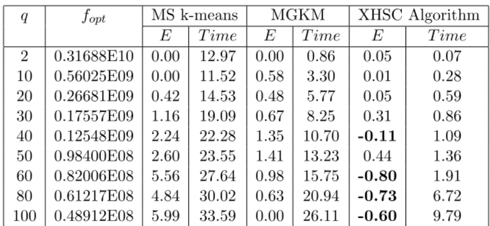
Table 1 presents the results for the TSPLIB-3038 data set. It exhibits the results produced by XHSC algorithm and, for comparison, those of two algo-rithms presented in Bagirov(2008). The first two columns show the number of clusters (q) and the best known value for the global optimum (fopt) taken from Bagirov(2008). The next columns show the error (E) for the best solution produced (fBest) and the mean CPU time (T ime) given in seconds associated to three algorithms: multi-start k-means (MS k-means), modified global k-means (MGKM) and the proposed XHSM. The errors are calculated in the following way: E = 100 (fBest−fopt)/ fopt.

The multi-start k-means algorithm is the traditional k-means algorithm with multiple initial starting points. In this experiment, to find q clusters, 100 times q starting points were randomly chosen in the MS k-means algorithm. The global k-means (GKM) algorithm, introduced by Likas et alli (2003), is a significant improvement of the k-means algorithm. The MGKS is an improved version of the GKM algorithm proposed by Bagirov(2008). The XHSM solutions were produced by using 10 starting points in all cases, except q = 40 and q = 50, where 20 and 40 starting points were taken, respectively.

q fopt MS k-means MGKM XHSC Algorithm

E T ime E T ime E T ime

2 0.31688E10 0.00 12.97 0.00 0.86 0.05 0.07 10 0.56025E09 0.00 11.52 0.58 3.30 0.01 0.28 20 0.26681E09 0.42 14.53 0.48 5.77 0.05 0.59 30 0.17557E09 1.16 19.09 0.67 8.25 0.31 0.86 40 0.12548E09 2.24 22.28 1.35 10.70 -0.11 1.09 50 0.98400E08 2.60 23.55 1.41 13.23 0.44 1.36 60 0.82006E08 5.56 27.64 0.98 15.75 -0.80 1.91 80 0.61217E08 4.84 30.02 0.63 20.94 -0.73 6.72 100 0.48912E08 5.99 33.59 0.00 26.11 -0.60 9.79

It is possible to observe in each row of Table 1 that the best solution produced by the new XHSC Algorithm becomes significantly smaller than that by MS k-means when the number of clusters q increases. In fact, this algorithm do not perform well for big instances, in despite being one of most used algorithms. Wu et alli (2008) present the top 10 data mining algorithms identified by the IEEE International Conference on Data Mining in December 2006. The k-means assumes the second place in this list. The comparison between XHSC and MGKM solutions demonstrates similar superiority of proposed algorithm. In the same way, the comparison of time columns shows a consistent speed advantage of proposed algorithm over the older ones.

On the other hand, the best solution produced by the XHSC Algorithm is very close to the putative global minimum, the best known solution of the TSPLIB-3038 instance. Moreover, in this preliminary experiment, by using a relatively small number of initial starting points, four new putative global minimum results (q = 40, q = 60, q = 80 and q = 100) have been established.

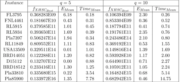
Instance q= 5 q= 10

f_XHSCBest E_{M ean} T ime_{M ean} f_XHSCBest E_{M ean} T ime_{M ean} FL3795 0.368283E09 6.18 0.18 0.106394E09 2.30 0.26 FNL4461 0.181667E10 0.43 0.31 0.853304E09 0.36 0.52 RL5915 0.379585E11 1.01 0.45 0.187794E11 0.41 0.74 RL5934 0.393650E11 1.69 0.39 0.191761E11 2.35 0.76 Pla7397 0.506247E14 1.94 0.34 0.243486E14 2.10 0.80 RL11849 0.809552E11 1.11 0.83 0.369192E11 0.53 1.55 USA13509 0.329511E14 0.01 1.01 0.149816E14 1.39 1.69 BRD14051 0.122288E11 1.20 0.82 0.593928E10 1.17 2.00 D15112 0.132707E12 0.00 0.88 0.644901E11 0.71 2.27 BRD18512 0.233416E11 1.30 1.25 0.105912E11 1.05 2.24 Pla33810 0.335680E15 0.22 3.54 0.164824E15 0.68 5.14 Pla85900 0.133972E16 1.35 7.78 0.682942E15 0.46 14.75

Table 2: Results for larger instances of the TSPLIB collection

Table 2 presents the computational results produced by the XHSC Al-gorithm for the largest instances of Symmetric Traveling Salesman Problem (TSP) collection: FL3795, FNL4461, RL5915, RL5934, Pla7397, RL11849, USA13509, BRD14051, D15112, BRD18512, Pla33810 and Pla85900. For each instance, it is presented two cases: q = 5 and q = 10. Ten dif-ferent randomly chosen starting points were used. For each case, the table presents: the best objective function value produced by the XHSC Algorithm (fXHSCBest), the average error of the 10 solutions in relation to the best

solu-tion obtained (EM ean) and CPU mean time given in seconds (T imeM ean). It was impossible to perform a comparison on given the lack of records of so-lutions of these instances . Indeed, the clustering literature seldom considers instances with such number of observations. Only a possible remark, the low

values presented in columns (EM ean) show a consistent performance of the proposed algorithm.

5

Conclusions

In this paper, the Extended HSC algorithm, a new method for the solu-tion of the minimum sum-of-squares clustering problem, has been proposed. The robustness performance of the XHSC Algorithm can be attributed to the complete differentiability of the approach. The speed performance of the XHSC Algorithm can be attributed to the partition of the set of observa-tions in two non overlapping parts. This last approach engenders a drastic simplification of computational tasks.

From the results presented in Tables 1 and 2, as well other results ob-tained for solving classical problems of the literature (see Sousa(2005)), it was possible to observe that the implementation of the XHSC algorithm reaches the best known solution, in most of the cases, otherwise calculates a solution which is close to the best. Moreover, some new best results in the cluster literature have been established, as these shown in the present paper for the TSPLIB-3038 instance.

Finally, it must be remembered that the MSSC problem is a global op-timization problem with a lot of local minima, so the algorithm only can produce local minima. However, the obtained computational results pre-sented a deep local minima property, perfectly adequate to the necessities and demands of real applications.

References

BAGIROV, A. M. and YEARWOOD, J. (2006) “A New Nonsmooth Op-timization Algorithm for Minimum Sum-of-Squares Clustering Problems”, European Journal of Operational Research, 170 pp. 578-596

BAGIROV, A. M. (2008) “Modified Global k-means Algorithm for Minimum Sum-of-Squares Clustering Problems”, Pattern Recognition, Vol 41 Issue 10 pp 3192-3199.

DUBES, R. C. and JAIN, A. K. (1976) “Cluster Techniques: The User’s Dilemma”, Pattern Recognition No. 8 pp. 247-260.

HANSEN, P. and JAUMARD, B. (1997) “Cluster Analysis and Mathemati-cal Programming”, MathematiMathemati-cal Programming No. 79 pp. 191-215.

HARTINGAN, J. A. (1975) “Clustering Algorithms”, John Wiley and Sons, Inc., New York, NY.

JAIN, A. K. and DUBES, R. C. (1988) “Algorithms for Clustering Data”, Prentice-Hall Inc., Upper Saddle River, NJ.

JAIN, A. K.; MURTY, M. N. and FLYNN, P. J. (1999) “Data Clustering: A Review”, ACM Computing Surveys, Vol. 31, No. 3, Sept 1999.

LIKAS, A.; VLASSIS, M. and VERBEEK, J. (2003) “The Global k-means Clustering Algorithm”, Pattern Recognition, Vol 36 pp 451-461.

SOUSA, L.C.F. (2005) “Desempenho Computacional do M´etodo de Agrupa-mento Via Suaviza¸c˜ao Hiperb´olica”, M.Sc. thesis - COPPE - UFRJ, Rio de Janeiro.

SP ¨ATH, H. (1980) “Cluster Analysis Algorithms for Data Reduction and Classification”, Ellis Horwood, Upper Saddle River, NJ.

WU, X. et alli (2008) “Top 10 Algorithms in Data Mining”, Knowledge and Information Systems, Vol 14 No. 1, pp 1-37

XAVIER, A.E. (1982) “Penaliza¸c˜ao Hiperb´olica: Um Novo M´etodo para Resolu¸c˜ao de Problemas de Otimiza¸c˜ao”, M.Sc. Thesis - COPPE - UFRJ, Rio de Janeiro.

XAVIER, A.E. (2008) “The Hyperbolic Smothing Clustering Method”, sub-mited to Pattern Recognition.