Summary Data from the Sixth AIAA Computational Fluid Dynamics Drag Prediction Workshop: Code Verification

Summary of Data from the Sixth AIAA CFD Drag

Prediction Workshop: Case 1 Code Verification

Christopher J. Roy 1

Virginia Tech, Blacksburg, VA, 24061, USA Christopher L. Rumsey 2

NASA Langley Research Center, Hampton, Virginia 23681-2199, USA Edward N. Tinoco 3

Retired, Kent, WA, 98031, USA

Results from the Sixth AIAA CFD Drag Prediction Workshop (DPW-VI), Case 1 Code Verification are presented. This test case is for the turbulent flow over a 2D NACA 0012 airfoil using Reynolds-Averaged Navier-Stokes (RANS) turbulence models. A numerical benchmark solution is available for the standard Spalart-Allmaras (SA) turbulence model that can be used for code verification purposes, i.e., to verify that the numerical algorithms employed are consistent and that there are no programming mistakes in the software. For the Case 1 code verification study, there were 31 data submissions from 16 teams: 23 with the SA model (using various versions), 4 with the omega SST model (two variants), and one each with kl, k-epsilon, an explicit algebraic Reynolds stress model, and the lattice Boltzmann method (LBM) with very large eddy simulation (VLES). Various grid types were employed including structured, unstructured, Cartesian, and adapted grids. The benchmark numerical solution was deemed to be the correct solution for the 21 submissions with the standard SA model, the SA-noft2 variant (without the ft2 term),

and the SA-neg variant (designed to avoid nonphysical transient states in discrete settings). While many of these 21 submissions did demonstrate first-order convergence on the finer meshes, others showed either nonconvergent solutions in terms of the aerodynamic forces and moments or converged to the wrong answer.

1 _{Professor and Assistant Department Head for Graduate Studies; [email protected]. AIAA Associate Fellow} 2 _{Senior Research Scientist, Computational AeroSciences Branch; [email protected]. AIAA Fellow} 3 _{Boeing Technical Fellow (Retired); [email protected]. AIAA Associate Fellow}

2

Results for this case highlight the continuing need for rigorous code verification to be conducted as a prerequisite for design, model validation, and analysis studies.

I. Nomenclature

CDp Pressure Drag Coefficient CDv Skin Friction Drag Coefficient CL Lift Coefficient

CMy Pitching Moment Coefficient (about the quarter chord) Cf Surface skin friction coefficient

Cp Surface pressure coefficient f General solution functional h Grid spacing = sqrt(1/N) N Number of grid points or cells

pˆ Observed order of accuracy r Grid refinement factor x Airfoil coordinate (chordwise) y Airfoil coordinate (normal to chord)

II. Introduction

HE AIAA CFD Drag Prediction Workshop (DPW) Series was initiated by a working group of members from the Applied Aerodynamics Technical Committee of the American Institute of Aeronautics and Astronautics. The primary goal of the workshop series was to assess the state-of-the-art of modern computational fluid dynamics methods using geometries and conditions relevant to commercial aircraft. From the onset, the DPW organizing committee has adhered to a primary set of guidelines and objectives for the DPW series:

3

• Assess state-of-the-art Computational Fluid Dynamics (CFD) methods as practical aerodynamic tools for the prediction of forces and moments on industry-relevant geometries, with a focus on absolute drag.

• Provide an impartial international forum for evaluating the effectiveness of CFD Navier-Stokes solvers.

• Promote balanced participation across academia, government labs, and industry.

• Use common public-domain subject geometries, simple enough to permit high-fidelity computations.

• Provide baseline grids to encourage participation and help reduce variability of CFD results. • Openly discuss and identify areas needing additional research and development.

• Conduct rigorous statistical analyses of CFD results to establish confidence levels in predictions. • Schedule open-forum sessions to further engage interaction among all interested parties.

• Maintain a public-domain accessible database of geometries, grids, and results.

• Document workshop findings; disseminate this information through publications and presentations.

Five workshops have been held prior to the present study, all held in conjunction with the AIAA Applied Aerodynamics Conference for that year. While there have been some variations, the workshops have typically used subjects based on commercial transport wing-body configurations – a consensus of the organizing committee based on a reasonable compromise between simplicity and industry relevance. The vast majority of the participants submit results generated with Reynolds Averaged Navier-Stokes (RANS) codes, although the organizing committee does not restrict the methodology. Further discussion of the Drag Prediction Workshop series can be found in Ref. [1].

A code verification exercise was also included in the fifth DPW [2]. There were three cases: 2D flat plate, 2D bump, and 2D NACA 0012 airfoil. Although most participants who ran these cases exhibited consistent results, the exercise identified problems with several model implementations. The NACA 0012 grids from that workshop were found to be too coarse to draw any conclusions, but this issue was addressed prior to the sixth workshop.

4 were optional.

Case 1 - Verification Study: 2D NACA 0012 Airfoil from the NASA Langley Turbulence Modeling Resource (TMR) [2] sponsored by the AIAA Fluid Dynamics Technical Committee Turbulence Model Benchmarking Working Group (TMBWG). Summary results for Case 1 are presented in this paper.

Case 2 - CRM Nacelle-Pylon Drag Increment: Calculate the drag increment between the CRM wing-body-nacelle-pylon (WBNP) and the CRM wing-body (WB) configurations. Flow conditions are: M = 0.85; Re = 5 million; fixed CL = 0.5 +/- 0.0001; Reference temperature = 100°F; aeroelastic deflections at the angle-of-attack 2.75 degrees geometry. Grid convergence study on Baseline WB and WBNP grids.

Case 3 - CRM WB Static Aero-Elastic Effect: Angle-of-attack sweeps are conducted using the aero-elastic deflections measured in the ETW Wind Tunnel Test. Flow conditions are: M = 0.85; Re = 5 million; Reference temperature = 100°F; Angle-of-attack sweep = [2.50, 2.75, 3.00, 3.25, 3.50, 3.75, 4.00] degrees. Use the Medium Baseline grids [7 solutions on 7 grids].

Case 4 - CRM WB Grid Adaptation [Optional]: Fixed lift condition for the CRM Wing-Body using an adapted grid family provided by the participant. Flow conditions are: M = 0.85; Re = 5 million; fixed CL = 0.5 +/- 0.0001; Reference temperature = 100°F; aeroelastic deflections at the angle-of-attack 2.75 degrees geometry. Start the adaptation process from the Tiny (or Coarse) Baseline Mesh. Participants are to document the adaptation process.

Case 5 - CRM WB Coupled Aero-Structural Simulation [Optional]: Fixed lift condition for the CRM Wing-Body coupled with computational structural analysis. Flow conditions are: M = 0.85; Re = 5 million; fixed CL = 0.5 +/- 0.0001; Reference temperature = 100°F; static aeroelastic deflections calculated, starting from the undeformed geometry. Use the Medium Baseline Grid. A structural FEM is supplied by NASA via the CRM Website. Modal shapes are also available.

The current paper summarizes the results for Case 1 only, which addresses code verification of the various CFD codes including the turbulence model used. The current code verification results include the

5

dimensionless force and moment coefficients as well as surface pressure and skin friction distributions. The summary results for Cases 2-5 are presented in Ref. [1] and a more detailed discussion of Case 5 is

presented in Ref. [3].

III.

Code Verification

Code verification has emerged as a rigorous technique for detecting errors related to software programming and numerical algorithms in CFD [4-6]. It is the first step in any design, analysis, or model validation study, and failure to successfully demonstrate that a code has been verified should lead one to view any results produced by the code with skepticism. Code verification provides confidence that the code will converge to the right solution and at the proper rate, the latter having a significant impact on solution cost given a specified numerical error tolerance. The most rigorous code verification test is either

comparison with an exact/known solution or use of Method of Manufactured Solutions [4-6] in conjunction with an order of accuracy test. The order of accuracy test determines whether or not the discretization error reduces at the expected rate with systematic mesh refinement. This test is equivalent to determining whether the observed order of accuracy (i.e., the order of accuracy that the solutions actually achieve) matches the formal order of accuracy of the given numerical scheme. For all discretization approaches (finite difference, finite volume methods, finite element, etc.), the formal order of accuracy can be obtained from a truncation error analysis. Since it is the most difficult test to satisfy (and therefore, the most

sensitive to coding mistakes and algorithm deficiencies), the order of accuracy test is the recommended acceptance test for code verification [4-6].

The observed order of accuracy is the accuracy that is directly computed from code output for a given simulation or set of simulations. The observed order of accuracy can be adversely affected by mistakes in the computer code, solutions which are not sufficiently smooth (i.e., contain singularities or

discontinuities), inconsistent numerical algorithms, and numerical solutions that are not in the asymptotic grid convergence range. When an exact solution is known, the observed order of accuracy can be found from

( )

6

where pˆ is the observed order of accuracy, fcoarse is the solution on the coarse grid, ffine is the solution on

the fine grid, and r is the grid refinement factor that measures how much the grid has been refined in each coordinate direction. It is important that the grids be systematically refined [4], which means that the grids must be refined by the same factor in each coordinate direction over the entire domain. It also requires that the mesh quality either stay the same or improve with mesh refinement.

IV.

Problem Description

The problem under consideration is the Mach 0.15 flow over a 2D NACA 0012 airfoil at a Reynolds number (based on the chord length) of 6 million, angle of attack of 10 degrees, and static temperature of 300 K. As shown in Figure 1, the outer boundary is located approximately 500 chord lengths away from the airfoil where fixed Riemann boundary conditions should be applied (i.e., without a point vortex circulation correction [7]). This problem has been used as a verification and validation test case and is available on the Turbulence Model Resource (TMR) web site [2]. The Spalart-Allmaras (SA) turbulence model [8,9] has been applied to this problem using both FUN3D and CFL3D, both of which have undergone rigorous code verification testing using the Method of Manufactured Solutions [10]. Since both of these codes have been demonstrated to converge to the same results, they have been used to establish a benchmark numerical solution for the SA turbulence model applied to this case [11]. Note that this benchmark solution is deemed appropriate for three variants of the SA model since the iteratively-converged results are the same in those cases: the baseline SA, SA without the ft2 term (SA-noft2), and the negative SA model (SA-neg). Except for possible numerical artifacts that can occur very near the trailing edge (depending on the grid and the particular numerical methods employed), the benchmark results for this case give fully attached flow. Some details from Ref. [11] are repeated below for completeness.

In this benchmark case, the definition of the NACA 0012 airfoil is slightly altered from the original definition so that the airfoil closes at the trailing edge (i.e., it has a sharp trailing edge). The reason for the sharp trailing edge was to make structured grid generation easier as well as to reduce the possibility of small-scale unsteadiness in the solutions. To close the trailing edge, the exact NACA 0012 formula

(

)

7

is used to create an airfoil between x=0 and x=1.008930411 (the T.E. is sharp at this location). Then the airfoil is scaled down by 1.008930411. Thus, the resulting airfoil is a perfect scaled copy of the 0012, with maximum thickness of approximately 11.894% relative to its chord (the original NACA 0012 has a maximum thickness of 12% relative to its blunted chord, but it, too, has a maximum thickness of 11.894% relative to its chord extended to 1.008930411). The revised airfoil definition is given by

(

)

On the airfoil surface, the boundary condition is a no-slip adiabatic solid wall condition, while at the outer boundary, a farfield Riemann boundary condition based on inviscid characteristic methods is employed (without the point vortex correction [7]). When solving the compressible RANS equations, the Prandtl number is taken to be Pr = 0.72, and the turbulent Prandtl number Prt = 0.90. Sutherland’s law for air is used for computing dynamic viscosity, and a calorically perfect gas is assumed. Details can be found on the TMR web site [2].Families of C-grids up to 14.7 million grid points are also available for download from this site. There are three C-grid families available: Family I, II, and III. Each family's finest grid has minimum spacing at the wall of 1 x 10-7_{c (where c is the chord length) and average stretching rate normal} to the wall of about 1.02 for the points near the wall. The leading edge spacing along the airfoil in all families is the same: 0.0000125c. The difference between the families is in their trailing edge streamwise spacing: 0.000125c for Family I, 0.0000125c for Family II, and 0.0000375c for Family III. The primary set of grids used in the current paper are from grid Family II, while some contributors employed grid Family I. An overview of these available Family I and Family II grids can be found in Figure 2. A few participants created their own NACA 0012 grids. However, there is no information available about them; it is not known how well they were constructed or whether successively refined grids are part of the same family. Therefore, results on participant-created grids should be viewed with caution.

A significant number of detailed solutions are provided on the TMR website, including surface pressure coefficient, surface skin friction coefficient, and a wide variety of flowfield line profiles. Lift and drag coefficients for three codes (FUN3D, CFL3D, and Tau) are shown in Figure 3 for the Family II set of

8

systematically-refined grids. This grid family has the finest streamwise spacing at the trailing edge compared with two other families available on the TMR website [2], and has been ascertained to provide the most accurate results. All grid families on the TMR web site are comprised of a systematic family of grids since the fine grid was generated initially and then each subsequent coarser grid was obtained by removing every other grid node in each direction (i.e., a grid refinement factor of r = 2).

In terms of grid-converged forces and pitching moment, the following values represent the estimated lower and upper bounds for the benchmark NACA 0012 solution from the CFL3D and FUN3D codes for the SA model and the variants SA-noft2 and SA-neg:

• CL = 1.0909 - 1.0911 • CD = 0.012270 - 0.012275 • CDp = 0.00606 - 0.00607 • CDv = 0.006205 - 0.006206 • CMy = 0.00676 - 0.00680

Thus, for example, the benchmark lift coefficient is “known” to within about 0.02% and drag coefficient to about 0.1%, or 1/10th _{of a drag count. There is a high degree of confidence in this benchmark solution since} both the CFL3D and FUN3D codes have undergone rigorous code order of accuracy testing using the Method of Manufactured Solutions [10], and a third independent code (Tau) also produces the same results.

V.

Results

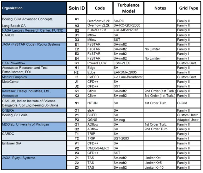
A summary of the contributions for Case 1 of the 6th _{Drag Prediction Workshop is given in Table 1.} There are 16 organizations using 17 different CFD codes, 6 different turbulence models (including 5 different variants of the SA turbulence model), and 6 different grid types including structured, unstructured, and Cartesian. Overall, there were 31 different contributions submitted.

9

Table 1. Summary of Contribution to Drag Prediction Workshop 6, Case 1

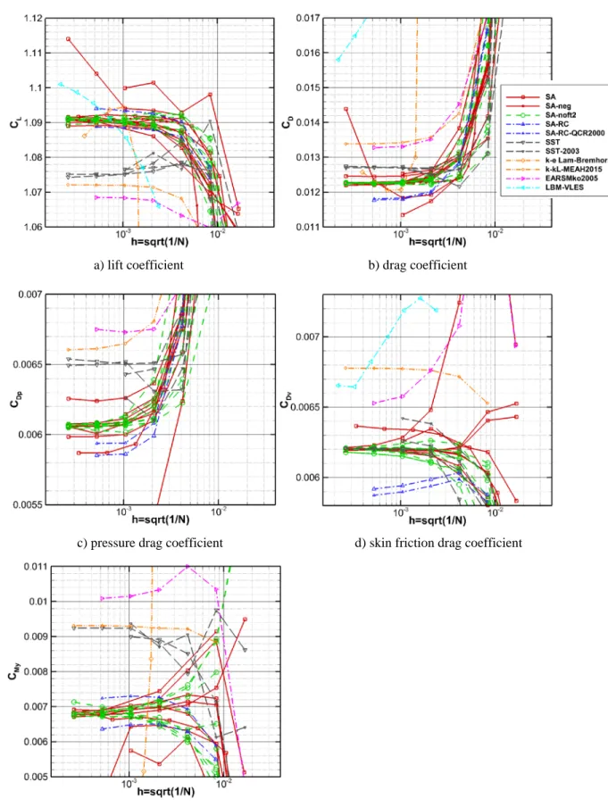
A. Results from All Contributors

The results for the force coefficients (lift, total drag, pressure drag, and skin friction drag) and moment coefficient about the quarter chord for all contributors are shown in Figure 4. All results are plotted versus h, a representative characteristic grid cell length for each grid level. The solutions on the right side of each plot are on grids as coarse as 113×33 nodes, while the solutions on the left (as h → 0) are as fine as 7169×2049 nodes. Since these combined results include all 6 turbulence models (and multiple variants of SA), they are not all expected to converge to the same answer. While most of the results do display a convergent behavior, showing up as asymptotic convergence with mesh refinement, a few outliers are nonconvergent on the finer meshes. It is possible that some of this nonconvergent behavior is due to incomplete iterative convergence, but we as organizers did not request sufficient information to assess the

10

level of iterative convergence of individual solutions. This missing information should be included in any future code verification cases, as incomplete iterative convergence can easily pollute the results, especially on the finer meshes.

Some general observations from Figure 4 are as follows. There appear to be two clusters of results for the lift and drag coefficients, likely due to different turbulence models. However, in both cases, there are also a few nonconvergent outliers on the finer meshes. For the moment coefficient, the data at zero indicates the contributor did not supply moment data, and one contributor likely had the wrong sign for the coefficient. Also, there appears to be significantly more scatter in the moment coefficient than in the force coefficients. Most of the results are grouped within 6 drag counts for the pressure drag and within 10 drag counts for the skin friction drag; however, again there are some outliers.

B. Effects of Turbulence Model

The results grouped by turbulence model are shown in Figure 5. The distribution of results with the different turbulence models and model variants are as follows:

• SA: 11 • SA-noft2: 9 • SA-neg: 3 • SA-RC: 1 • SA-RC-QCR2000: 1 • SST: 3 • SST-2003: 1 • k-ε Lam-Bremhorst 1 • k-kl: 1 • LBM-VLES: 1 • EARSM: 1

For all coefficients, the Lattice Boltzman Method (LBM) converges very slowly. For the lift coefficient, the SA and SST models seem to converge to approximately 1.09 and 1.075, respectively. Most SA model variants tend to converge to around CD = 0.01225 except the SA-RC variants, which seem to converge to 0.0118, a 4.5 drag count difference. The SST models converge to approximately 0.01275, a 5 drag count difference from the bulk of the SA models. The moment coefficient again shows a wider scatter than lift or total drag, with most SA results converging to near 0.0068, while the SST and k-kl models both converge to near 0.0093. For the pressure drag, most SA model variants converge to approximately 0.0061, with the

11

SA-RC variants converging a bit lower. Most SST and the k-kl models converge near 0.0065, a 4 drag count difference from the bulk of the SA models. For the skin friction drag, most models appear to be converging to approximately 0.0062 except the SA-RC model, which comes in a bit lower at 0.0059, and the k-kl model, which converges to 0.0068.

C. Effects of Grid Type

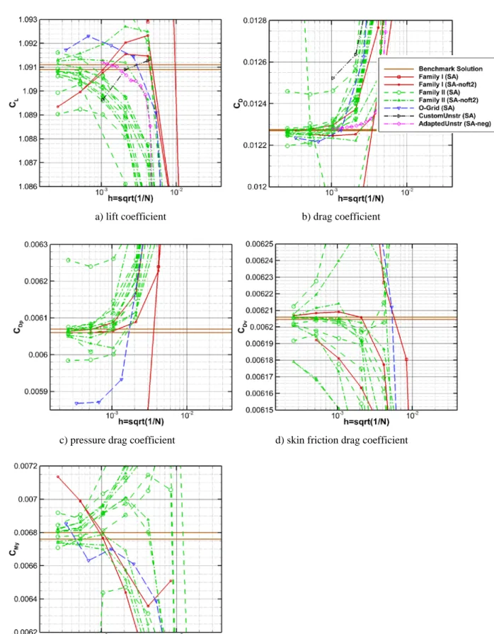
The results filtered by grid type are only given for the SA model variants where the benchmark numerical solution is expected to be appropriate (i.e., SA, SA-noft2, and SA-neg). The other models were excluded to ensure that we are truly looking at the effects of grid type and not just variations due to different turbulence models. The grid types shown in Figure 6 include Family I (3 submissions), Family II (15 submissions), one O-grid, one custom unstructured grid, and one adapted unstructured grid.

For the lift coefficient, the three contributions using grid Family I (with the trailing edge streamwise spacing coarser than Family II by a factor of 10) do not converge to the benchmark solution range, which is shown as the two horizontal maroon lines straddling CL = 1.091. The Family II submissions generally do seem to converge near the benchmark result, with a few outliers. The O-grid shows a nonmonotone behavior on the finest three meshes, but may be converging to the benchmark result; more grid levels are needed. The custom unstructured grid result is nonconvergent, but the adapted unstructured result appears to yield results close to the correct result on significantly coarser grids than the (unadapted) Family II submissions.

For the drag coefficient, most results appear to converge to the benchmark drag result except for one of the three Family I submissions, two of the Family II submissions, and the custom unstructured submission. The adapted unstructured approach appears to converge to the benchmark result on fairly coarse meshes (at least as judged by total node count). The O-grid results are 2 drag counts lower than the benchmark solution for pressure drag and 2 drag counts higher than the benchmark solution for skin friction drag, thus explaining the correct total drag being predicted on the O-grid. The two unstructured contributions did not provide a drag breakdown to pressure and skin friction components (and thus, show up with values of zero). Two of the Family I submissions and all but two of the Family II submissions seem to converge to the benchmark solution for both pressure and skin friction drag.

12

For the moment about the quarter chord, the Family I submissions do not converge to the benchmark result, while the grid Family II submissions do generally converge to the benchmark solution (with one or two exceptions). The O-grid is again nonmonotone on the finest grids and it is not clear to what value of moment coefficient it is converging.

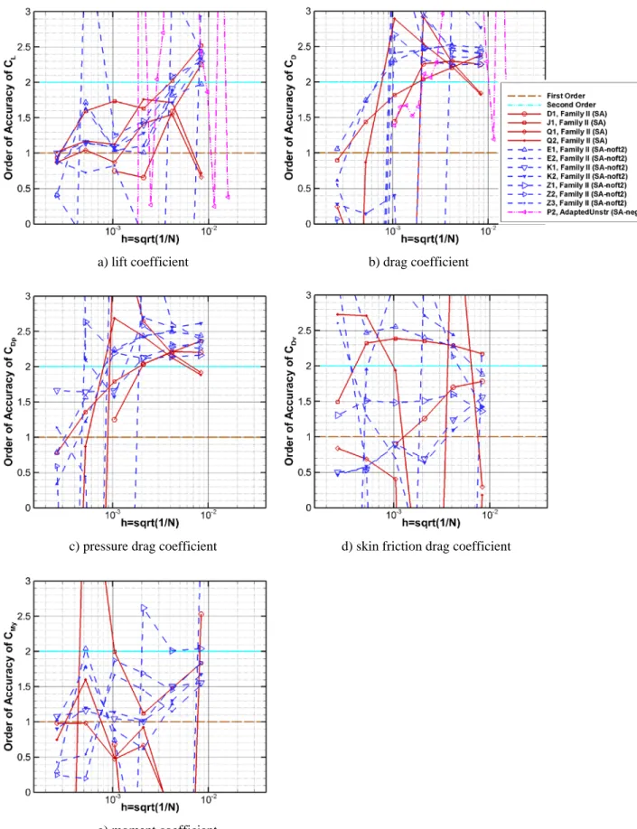
D. Order of Accuracy

The order of accuracy is given in Figure 7 for the SA models where the benchmark numerical solution is expected to be appropriate (i.e., the SA, SA-noft2, and SA-neg). Note that since the Family I grids, the O grid, the unstructured grid, and cases H1, O1, V1, and V2 were all shown to be nonconvergent in the last section, they were not included.

Since the benchmark numerical solution was demonstrated to be correct with multiple CFD codes that have undergone rigorous code verification using the Method of Manufactured Solutions [10], the

benchmark results can be used to conduct a code verification exercise with these remaining 12 submissions. For the plots shown in Figure 7, the exact solution was taken to be the mean of the interval given for each coefficient given above. While not technically correct (since the true exact solution is only assumed to be somewhere within the interval), this approach at least makes the plots readable versus computing order of accuracy with both the upper and lower bounds of the benchmark numerical solution. The order of accuracy is computed as discussed earlier in Section III. Note that an order of accuracy of zero indicates that coefficient was not included in the data submission, which occasionally occurred for Cy, CDp, and CDv.

Most of the Family II submissions display orders of accuracy between first and second order, although they are convergent at first order on the finest meshes. While all of the codes are nominally second-order accurate (except for four submissions that identified as first order for the SA turbulence equation), a reduction in the order of accuracy down to first order is not surprising due to the presence of the strong trailing edge singularity as well as the weaker stagnation point singularity near the leading edge. The Family I submissions are generally not convergent, although one submission appears to be convergent at second order except on the finest mesh (true for CD, CDp, and CDv). The custom unstructured result appears to be convergent for the drag coefficient only (note that drag components were not included in this submission). The adaptive unstructured result is shown on the figures, but the order of accuracy results are

13

only approximate since the grid is not systematically refined [4].

The lift and moment coefficients for the Family II submissions appear to be the best behaved, with the drag and drag component results showing more scatter on the finest meshes. This is quite possibly due to the use of the mean of the drag range being used for the “exact solution” in the observed order of accuracy computation.

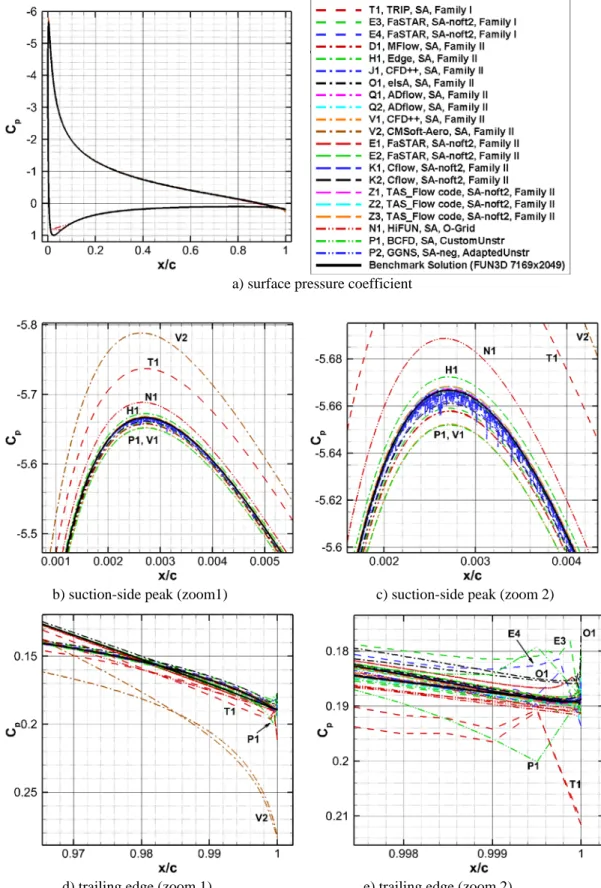
E. Surface Distributions

The pressure coefficient along the surface of the airfoil is given in Figure 8 for all contributors. For this and all following surface distribution figures, additional information is included in the legend to try to help the reader discern trends and isolate reasons for differences between results. While nearly all of the submissions show very similar profiles (see Figure 8a), a closer inspection of the suction (top) side peak shown in Figure 8b and c identifies a number of outliers. The T1 submission displays unusual behavior near x/c = 0.012, which may be due to transition from laminar to turbulent flow. Submissions V2, T1, and I2 all appear to predict higher peaks (lower pressures), but the I2 submission does not provide sufficient

resolution to know for sure. The Lattice Boltzmann solver (G1) is noisy as expected. The EARSM model (H2) predicts the lowest suction peak. Most of the submissions that predict higher or lower suction peaks also predict lower or higher trailing edge pressure, respectively (see Figure 8d and e). The A1, A2, T1, and T2 submissions all display some oscillations near the trailing edge.

The pressure coefficient for the SA models where the benchmark numerical solution is expected to be appropriate (i.e., the SA, SA-noft2, and SA-neg) are given in Figure 9. A number of submissions (N1, T1, V1) overpredict the suction peak, while P1 and V1 underpredict it. Most of the submissions cluster closely to the benchmark numerical solution obtained using FUN3D on an extremely fine 7169×2049 Family II mesh. Most of the submissions match reasonably well to the benchmark solution at the trailing edge, with the notable exception of submission V2.

There are significantly more differences observed in the skin friction coefficient for all the submissions, as shown in Figure 10. Note that a number of contributors were omitted from the skin friction analysis due to problems with the data ordering (N1), skin friction coefficient scaling (O1), surface geometry resolution (I2), or the fact that Cf,x was provided rather than Cf (B2, H1, H2, and P2). Numerous submissions (e.g.,V2,

14

T1) appear to predict laminar flow near the leading edge and then transition to turbulent flow downstream. The participants were instructed to run the cases fully turbulent. The Lattice Boltzmann method and, to a lesser extent, the SST-2003 model, predict higher peak skin friction values. The V2 submission appears to be an outlier at both the suction peak and at the trailing edge. The two SST model results (D3 and V3) show good agreement with each other. The submissions on grid Family I show increases in the skin friction near the trailing edge.

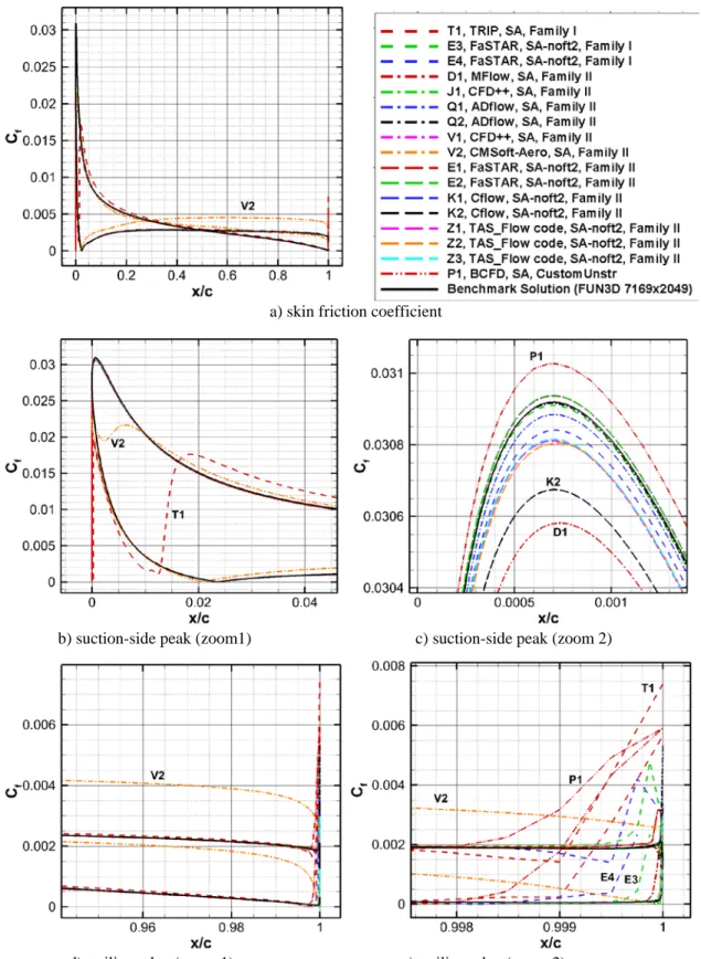
The skin friction coefficient for the SA models where the benchmark numerical solution is expected to be appropriate (i.e., the SA, SA-noft2, and SA-neg) are given in Figure 11, along with the numerical benchmark solution (FUN3D on a 7169×2049 Family II grid). Submissions T1 and V2 are clearly outliers, possibly due to their prediction of late transition from laminar to turbulent flow on the upper surface. Submission P1 overpredicts the peak skin friction, while D1 and K2 underpredict it. A large peak in skin friction occurs at the trailing edge for those submissions on the Family I grid.

VI.

Conclusions

An analysis of the results for the 2D code verification case yielded the following conclusions. Most SA variants on the Family II grids do appear to be converging to the benchmark numerical solution. However, this convergence is generally only first-order accurate on the finer meshes, even though the codes are all nominally second-order accurate. The reason is likely the strong trailing edge singularity, which has a locally first-order convergence and eventually pollutes the entire solution over the domain since the mathematical character of the flow is elliptic. Three of the four SST model results appear to be converging to the same result. However, as none of these codes have been rigorously verified using the Method of Manufactured Solutions, this agreement is not yet sufficient to establish a numerical benchmark solution for the SST model.

The grid used is important. The results on grid Family II were generally much better than those on grid Family I, with the only difference between these two grids being the trailing edge streamwise spacing is a factor of ten finer for Family II. This finding suggests that it is critical to resolve the trailing edge

singularity. The single submission that employed unstructured adaptive grids showed promising results, with the solutions approaching the benchmark values at much lower node counts than the unadapted grids.

15

Other participant-generated grids generally gave less accurate results than the provided Family II grids, but the reasons were not clear.

Examination of the surface distributions suggests that some of the submissions predicted a delayed transition from laminar to turbulent flow on the upper airfoil surface. This delayed transition should not occur for the SA model for this case, if used as specified by the model developers. An implementation error is likely. For example, it is possible that the freestream turbulence in these transitional solutions has been set below the recommended level. In addition, the Family I grid submissions generally predicted a large skin friction peak at the trailing edge, which is clearly incorrect, at least for the SA models where the benchmark solution is appropriate.

For the outlier submissions that were nonconvergent, nonmonotone on the finer grids, or converged to the wrong answer, it is unclear what the source of the problem is. A more transparent reporting of iterative convergence may have shed some light on the source of this problem and should be implemented in future workshops. Other likely sources could be: 1) a software coding mistake, 2) an improper boundary condition used, 3) an incorrect wall distance used in the turbulence model, 4) the presence of round-off error if run in single precision, and 5) incorrect variant of the model reported. While the ideal approach to code

verification is to demonstrate order of accuracy using the Method of Manufactured Solutions, this numerical benchmark solution allows an easier path to code verification that does not require the code intrusiveness of Manufactured Solutions. Code verification should be considered a prerequisite for application of a code to design, model validation, and analysis.

Acknowledgments

The authors would like to thank the entire 6th _{Drag Prediction Workshop committee for their dedication} and hard work over the past two years. We would also like to thank all of the contributing groups for their submissions, without which this paper would not be possible.

16

References

1. Tinoco, E. N., Brodersen, O. P., Keye, S., Laflin, K. R., Feltrop, E., Vassberg, J. C., Mani, M., Rider, B., Wahls, R.,

Morrison, J. H., Hue, D., Gariepy, M., Roy, C. J., Mavriplis, D. J., and Murayama, M., “Summary of Data from the

Sixth AIAA CFD Drag Prediction Workshop: CRM Cases 2 to 5,” AIAA Paper 2017-1208, January 2017.

2. Levy, D. W., Laflin, K. R., Tinoco, E. N., Vassberg, J. C., Mani, M., Rider, B., Rumsey, C. L., Wahls, R., Morrison,

J. H., Brodersen, O. P., Crippa, S., Mavriplis, D. J., and Murayama, M., “Summary of Data from the Fifth

Computational Fluid Dynamics Drag Prediction Workshop,” Journal of Aircraft, Vol. 51, No. 4, 2014, pp.

1194-1213.

3. NASA Langley Turbulence Modeling Resource web site, 2D NACA 0012 Airfoil Validation Case:

https://turbmodels.larc.nasa.gov/naca0012numerics_val.html (last accessed 9/25/2017).

4. Keye, S. and Mavriplis, D., “Summary of Data from the Sixth AIAA CFD Drag Prediction Workshop: Case 5

(Coupled Aero-Structural Simulation),” AIAA Paper 2017-1207, January 2017.

5. Oberkampf, W. L. and Roy, C. J., Verification and Validation in Scientific Computing, Cambridge University Press,

Cambridge, 2010.

6. Roache, P. J., Fundamentals of Verification and Validation, Hermosa Publishers, New Mexico, 2009.

7. Roy, C. J., “Review of Code and Solution Verification Procedures for Computational Simulation,” Journal of

Computational Physics, Vol. 205, No. 1, 2005, pp. 131-156.

8. Thomas, J. L. and Salas, M. D., “Far-Field Boundary Conditions for Transonic Lifting Solutions to the Euler

Equations,” AIAA Journal, Vol. 24, No. 7, 1986, pp. 1074-1080.

9. Spalart, P. R. and Allmaras, S. R., “A One-Equation Turbulence Model for Aerodynamic Flows,” Recherche

Aerospatiale, No. 1, 1994, pp. 5-21.

10.Allmaras, S. R., Johnson, F. T., and Spalart, P. R., “Modifications and Clarifications for the Implementation of the

Spalart-Allmaras Turbulence Model,” ICCFD7-1902, 7th International Conference on Computational Fluid

Dynamics, Big Island, Hawaii, 9-13 July 2012.

11.Rumsey, C. L. and Thomas, J. L., “Application of FUN3D and CFL3D to the Third Workshop on CFD Uncertainty

Analysis,” NASA/TM-2008-215537, November 2008.

12.AIAA Committee on Standards in CFD, “AIAA Standard for Code Verification in Computational Fluid Dynamics,”

17 Figures

Figure 1. Domain and boundary conditions for Case 1: NACA 0012, M = 0.15, Rec = 6 million (c=1), Tref = 540 R (adapted from Ref. [2]).

18

a) Family II grid (449×129), far view b) Family II grid (449×129), near view

c) Family II grid (449×129), trailing edge d) Family I grid (449×129), trailing edge

19

20

a) lift coefficient b) lift coefficient (zoomed)

c) drag coefficient d) drag coefficient (zoomed)

21

g) pressure drag coefficient h) pressure drag coefficient (zoomed)

i) skin friction drag coefficient j) skin friction drag coefficient (zoomed)

22

a) lift coefficient b) drag coefficient

c) pressure drag coefficient d) skin friction drag coefficient

e) moment coefficient

23

a) lift coefficient b) drag coefficient

c) pressure drag coefficient d) skin friction drag coefficient

e) moment coefficient

24

a) lift coefficient b) drag coefficient

c) pressure drag coefficient d) skin friction drag coefficient

e) moment coefficient

Figure 7. Order of accuracy computed using the middle of the benchmark numerical solution interval by grid type for SA, SA-noft2, and SA-neg contributors.

25

a) surface pressure coefficient

b) suction-side peak (zoom1) c) suction-side peak (zoom 2)

d) trailing edge (zoom 1) e) trailing edge (zoom 2)

26

a) surface pressure coefficient

b) suction-side peak (zoom1) c) suction-side peak (zoom 2)

d) trailing edge (zoom 1) e) trailing edge (zoom 2)

27

a) skin friction coefficient

b) suction-side peak (zoom1) c) suction-side peak (zoom 2)

d) trailing edge (zoom 1) e) trailing edge (zoom 2)

28

a) skin friction coefficient

b) suction-side peak (zoom1) c) suction-side peak (zoom 2)

d) trailing edge (zoom 1) e) trailing edge (zoom 2)