Three Essays in Labor and Education Economics

(1)

Three Essays in Labor and Education Economics

by

Breno Braga

A dissertation submitted in partial fulllment of the requirements for the degree of

Doctor of Philosophy (Economics)

in the University of Michigan 2014

Doctoral Committee:

Professor John Bound, Co-Chair Professor Charles Brown, Co-Chair Professor David Lam

(2)

c

(3)

DEDICATION

(4)

ACKNOWLEDGMENT

I am very grateful to my dissertation committee, John Bound, Charlie Brown, David Lam and Brian McCall, for all the comments and suggestions that improved this dissertation signicantly. I am especially thankful to John and Charlie for the many hours of discussion and endless constructive comments on my work. Both of them have hugely inuenced the way I think about economics and conduct my research.

The second chapter of this dissertation is a joint work with Paola Bordon and the third chapter is a joint work with John Bound, Joe Golden and Gaurav Khanna. I am very grateful to all these coauthors from whom I have learned much throughout our time together. I wish to thank all my colleagues in the Economics PhD program, in particular Aditya Aladangady, Vanessa Alviarez, Lasse Brune, Sebastian Calonico, Italo Gutierrez, Monica Hernandez, Cynthia Doniger and Peter Hudomiet. They were an incredible source of aca-demic and personal support and I deeply appreciate all their suggestions.

I am continually thankful for my beautiful girlfriend, Katherine Axelsen. In addition to proofreading all my papers, her kindness and love provided great happiness to me these past 4 years. I could not have a better partner to take the next step of my life.

(5)

Therez-love were always present during my work and crucial to all my accomplishments.

Last, but denitely not least, I would like to deeply thank my parents Nize and Antonio Braga. Since an early age they have been obsessed with providing my sister and I with the best possible education despite many adverse situations. This dissertation is nothing but the successful result for their tireless eorts.

(6)

LIST OF TABLES

1.1 Literature Review . . . 46

1.2 Work History Variables . . . 47

1.3 Descriptive Statistics . . . 48

1.4 The Eect of Schooling, Experience, and Career Interruptions on Earnings . 49 1.5 The Eect of Schooling, Experience, and Career Interruptions on Earnings, Other Demographic Groups . . . 50

1.6 The Eect of Schooling, Experience, and Career Interruptions on Earnings -Leaving School Year as First Year a Responded Left School . . . 51

1.7 The Eect of Unemployment and Schooling on Earnings by Timing of Unem-ployment . . . 52

1.8 The Eect of Schooling, Experience, and Career Interruptions on Earnings, Individual Fixed Eect . . . 53

2.9 Descriptive Statistics for Selective and Non-Selective Universities . . . 89

2.10 Earnings for Selective and Non-Selective Universities . . . 89

(10)

2.12 EL-SD Regression Discontinuity Test - Robustness Checks . . . 91 3.13 Fraction of Computer Scientists and Immigrants in the US Workforce by

Oc-cupation . . . 136 3.14 Calibrated Parameters . . . 137 3.15 Summary of Results from Counterfactual Simulation . . . 138

(11)

LIST OF FIGURES

1.1 Employment Attachment over the Life-Cycle - High School Graduates . . . 54

1.2 Employment Attachment over the Life-Cycle - BA or More Graduates . . . . 55

1.3 Earnings Coecient on Schooling by Work Experience Groups . . . 56

1.4 Earnings Coecient on Schooling by Cumulative Years Unemployment Groups 57 1.5 Earnings Coecient on Schooling by Cumulative Years OLF Groups . . . 58

1.6 Log Earnings - Work Experience Prole . . . 59

1.7 Log Earnings - Cumulative Years Unemployed Prole . . . 60

1.8 Log Earnings - Cumulative Years OLF Prole . . . 61

1.9 The Eect of Unemployment on Earnings by Timing of Unemployment . . . 62

1.10 The Eect of OLF on Earnings by Timing of OLF periods . . . 63

1.11 High Type Belief . . . 64

2.12 Application Process to Traditional Universities . . . 92

2.13 Smoothed Language PAA Score Distribution . . . 92

(12)

2.15 Graduation from Selective University Discontinuity . . . 94

2.16 Discontinuity at Pre-treatment Outcomes . . . 95

2.17 Earnings Discontinuity by Experience . . . 96

3.18 Major Trends (1990 to 2012) . . . 139

3.19 H-1 and H-1B Visa Population . . . 140

3.20 Model and Counterfactual (1/2) . . . 141

(13)

CHAPTER I

Schooling, Experience, Career Interruptions, and

Earnings

1.1 Introduction

Economists have long recognized that schooling and experience are two of the most important aspects of earnings determination.1 _{Given the importance of these two variables, a natural}

question is: how does their interaction aect earnings? In other words, do educated workers have a higher or lower wage increase as they accumulate experience? Which theories can explain this relationship?

In addition to the time spent at work, it is also well documented that individuals spend a signicant portion of their time unemployed or out of the labor force during their careers, and these events have a persistent eect on a worker's life-time earnings.2 _{Given the importance}

of non-working events throughout a worker's life cycle, it is also of considerable interest to

1_{The study of the impact of schooling and experience on earnings goes back to Becker (1962), Mincer}

(1962) and Ben-Porath (1967).

2_{Examples of papers studying the eect of career interruptions on earnings include Mincer and Polachek}

(1974), Corcoran and Duncan (1979), Mincer and Ofek (1982), Kim and Polachek (1994), Light and Ureta (1995), and Albrecht et al. (1999).

(14)

investigate whether educated workers suer greater or lower wage losses after out-of-work periods.

It is within this context that this paper examines how the interaction between schooling and work experience aects earnings. In contrast to the existing literature, I take into consideration that workers spend a signicant amount of time not employed throughout their careers and that working and non-working periods are substantially dierent in terms of the interaction between workers and rms.

While considering the dierence between working and non-working periods seems natural, this dierence has been ignored in most of the existing literature. Table 1.1 presents some the most important papers that have addressed how the interaction between schooling and experience aects earnings. As can be seen in the table, in order to identify whether more educated workers have a higher or lower wage increase with experience, these papers have used rough measures of experience, such as age minus schooling minus six or years since transition to the labor force.3

As seen in the table, the overall nding in the literature is that returns to potential experience do not change across educational groups in old datasets (Mincer, 1974), or decrease with educational level in the most recent datasets (Lemieux, 2006 and Heckman et al., 2006).4

These results had a lasting inuence on empirical work in the eld of labor economics. For example, Mincer (1974) used his ndings to justify the separability between schooling and

3_{Note also that these studies dier on how they dene earnings. For example, Farber and Gibbons (1996)}

use earning in levels. There is also a dierence between using annual or hourly wages as the dependent variable. Mincer (1974) uses annual earnings, but only nds evidence for parallel wage prole when controlling for weeks worked in the past calendar year. With the exception of Heckman et al. (2006), most recent papers have used hourly earnings as the dependent variable.

4_{Altonji and Pierret (2001) also nd negative coecients for interaction between schooling and experience}

when including ability measures not observed by rms that are correlated to schooling on the earnings equation.

(15)

experience present in the Mincer earnings equation, which has remained for decades the ``workhorse'' of empirical research on earnings determination.5

Despite the unquestionable value of the articles presented in table 1.1, in this paper I point out issues associated with the measures of experience they use. The rst contribution of this paper is to demonstrate that potential experience used in Mincer (1974) confounds the impact of two distinct events on earnings: actual experience and past non-working periods. Furthermore, I demonstrate that if educated workers suer greater wage losses after out-of-work periods, potential experience can produce greater bias to the returns to experience for more educated workers.

This result is at odds with the literature that discusses the bias associated with using po-tential experience variable (Filer, 1993, Altonji and Blank, 1999, and Blau and Kahn, 2013). According to this literature, potential experience generates lower bias to the returns to expe-rience for demographic groups with higher employment attachment, such as more educated workers. In contrast, I demonstrate that potential experience can generate a greater bias to the returns to experience for workers with higher employment attachment if their earnings are more aected after career interruptions. To my knowledge, this is the rst paper that addresses this matter.

The second contribution of this paper is to use the National Longitudinal Survey of Youth (NLSY) to estimate a model where earnings depend on work experience, past unemploy-ment and non-participation periods, and their interaction with schooling. While there is an

5_{The existing literature presents some possible explanations for the non-increasing eect of schooling}

on earnings. In the traditional Mincerian model, all workers have the same rate of returns to on-the-job investment, that is independent of their educational achievement. This independence between human capital investments at school and on-the-job can justify the parallel log earnings-experience proles across educational groups. On the other hand, Farber and Gibbons (1996), and Altonji and Pierret (2001) claim that schooling is used by employers as a signal of a worker's ability. Therefore, schooling should not become more important for earnings as a worker accumulates work experience.

(16)

extensive literature the analysis the impact of career interruptions on earnings (Mincer and Polachek, 1974 and Mincer and Ofek, 1982), on the gender gap (Kim and Polachek, 1994 and Light and Ureta, 1995), and on race wage gap (Antecol and Bedard, 2004), to my knowledge this is the rst paper that addresses how past working and non-working periods aect the wage coecient on schooling.

The results from the estimation of the earnings model that fully characterize the work his-tory of individuals are remarkably dierent from the standard specication using potential experience. Using my preferred estimation method, I nd that for non-black males, the wage coecient on schooling increases by 1.8 percentage points with 10 years of actual experience, but decreases by 2.2 percentage points with 1 year of unemployment. In other words, the earning dierential between the more and less educated workers mildly rises with actual ex-perience but signicantly falls with unemployment. The periods a worker spends out of the labor force (OLF) do not signicantly aect the wage coecients on schooling. I also nd qualitatively similar results for blacks and women, with the exception that I nd a negative eect of the interaction between OLF periods and schooling on earnings for women.

I provide several robustness checks for these results. First, I estimate a non-parametric model where I do not impose restrictions on the relation between earnings, schooling, work experience, and career interruptions. Second, I change the earnings model so that the timing of career interruptions can also change the eect of schooling on earnings. Third, I take into consideration the possible endogeneity of work history, and estimate a model using an individual xed eect assumption. In all these specications, I consistently nd that more educated workers have a higher wage increase with work experience but suer greater wage losses after unemployment periods.

(17)

rationalize the empirical ndings of this paper. In the model, the productivity of a worker depends on his ability, schooling level and work experience. However, dierent from the articles in table 1.1, I assume that ability is complementary to schooling and experience in determining a worker's productivity. In other words, high ability workers have higher returns to human capital investments at school and on-the-job.

The model also shares features with the employer learning literature (Farber and Gibbons, 1996 and Altonji and Pierret, 2001). Firms observe schooling and the work history of individ-uals but have imperfect information about their ability. Within this framework, employers have to make predictions about a worker's ability using the information available at each period. As low-ability workers are more likely to be unemployed throughout their careers, rms use information regarding past employment history of workers in the prediction of their unobservable ability.6

Based on the framework described above, the model can predict the empirical results of the paper. The intuition is as follows. High ability workers learn faster on-the-job and have a higher productivity growth as they accumulate work experience. As ability and education are positively related, the model predicts that educated workers have a higher wage increase with experience. In addition, employers use past unemployment as a signal that a worker is low ability. As low ability workers have lower returns to schooling, the model predicts that more educated workers suer greater wage losses when their low ability is revealed through unemployment.

The paper is organized as follows. In section 2, I discuss the issues of using potential experience when estimating a typical Mincer equation if career interruptions have an impact

6_{While there are studies where employers use lay o information (Gibbons and Katz, 1991) or the duration}

of an unemployment spell (Lockwood, 1991 and Kroft et al., 2013) to infer a worker's unobservable quality, in this paper rms take into consideration the full work history of an individual.

(18)

on earnings. In section 3, I describe the data and I show some descriptive statistics. Section 4 presents the main empirical results of the paper, and I provide some robustness checks. In section 5, I describe the model, and Section 6 concludes the paper.

1.2 Potential Experience and Career Interruptions in the

Mincer Equation

The Mincer earnings equation has long been long used as the workhorse of empirical research on earnings determination. Based on theoretical and empirical arguments, Mincer (1974) proposed a specication where the logarithm of earnings is a linear function of education and a quadratic function of potential experience (age minus schooling minus six). Mincer also suggested that schooling and experience are separable in the earnings equation, meaning no interaction term between these two variables is required in the earnings equation. Notably, as discussed shown in table 1.1, Mincer founds evidence that potential experience proles are nearly parallel across educational groups.

There is wide discussion on the potential pitfalls with the earnings specication proposed by Mincer (Murphy and Welch (1990) and Heckman et al. (2006)), including discussion of the issues associated with using the potential experience variable (Filer, 1993 and Blau and Kahn, 2013). In addition to the existing critiques, in this section I discuss new issues with using the potential experience variable when non-working periods aect earnings.

In order to give some perspective to this issue, I begin the analysis with the traditional case where earnings are aected only by actual experience and not by non-working periods.7 _The

(19)

log-earnings generating process of workeri at time periodt (lnwit) with level of schoolings is dened by the equation below. The parameter βs

1 identies the impact of the increase of

actual experience for workers with level of education s.

lnwit =β0s+β1sexperit+εit (1.1)

For expositional purposes, and dierent from Mincer's suggested specication, I assume that log earnings are a linear function of experience. As discussed in Regan and Oaxaca (2009), an inclusion of a quadratic and cubic term tends to exacerbate the type of bias that is discussed here.8

The object of interest of the paper is the interaction between schooling and experience. In terms of the equation above, I am interested in how the parameter βs

1 changes across

dierent educational groups. Note that according to Mincer (1974) original specication, log-experience proles are parallel across educational groups: β₁s =β1 for all s.

Equation (1.1) describes how log-earnings changes with actual experience, but individuals can spend some time not working after they leave school. I denelτ i as an indicator variable that assumes a value of one if individualiworked at past time periodτ. The actual experience

variable is dened by the sum of past working periods after a worker left school:

experit =Pt

−1 τ=gliτ

whereg is the time at which an individual leaves school. I also assume thatliτ is independent of the wage error term εit and E[liτ] =ps, whereps is a constant between zero and one that 8_{In the empirical section of the paper I include dierent functional forms for both actual experience and}

(20)

indicates the expected fraction of periods that a worker with s level of education stays

employed after leaving school.9

In most datasets it is not possible to identify an individual's work history. For this reason, researchers have long used rough measures of experience which do not distinguish working and non-working periods, such as the potential experience variable. In the context described above, the potential experience variable pexpit, is dened as the time period since an indi-vidual left school:10

pexpit= t−1−g

In this framework, it is easy to show that the coecient that expresses how earnings change with potential experience is a biased estimator of βs

1, such that βe_pex = p_sβ₁s. In fact, this

is typical attenuation bias associate with using the potential experience variable present in the literature (Filer, 1993 and Blau and Kahn, 2013). Note that while potential experience attenuates the returns to experience for all demographic groups, the attenuation bias is higher for demographic groups with lower employment attachment. That is the reason why using complete measures of actual experience is a special issue in the literature that studies the gender wage gap (Altonji and Blank, 1999).

Note that as educated workers tend to have a higher employment attachment than uned-ucated workers, such that ps > ps−1, this model predicts that potential experience

under-estimates the dierence in the wage growth between educated and uneducated workers. In other words, if earnings are not aected by career interruptions, the potential experience

9_{A discussion of the potential endogeneity of}_liτ _{is found in section 1.3.2.}

10_{Mincer (1974)'s denition of age-6-schooling would also generate an error term regarding the correct}

(21)

generates a lower bias to the returns to experience for more educated workers. However, as I will show in section 1.3.2, this is the opposite to what it is observed in the data.

Suppose now that in addition to actual experience, non-working periods also have a long-term impact on wages.11 _{A representation for the earnings equation in this framework would}

be:

lnwit =β0s+β s

1experit+β2sinterrit+εit (1.2)

whereinterit is a measure of career interruptions of a worker since leaving school. Using the same notation as before, I dene career interruptions as the accumulation of non-working periods since an individual left school:

interrit=Pt

−1

τ=g(1−liτ)

Note that for simplicity, I assume that earnings are aected by the cumulative non-working periods. However, one can argue that the order and length of non-working periods have a dierent impact on earnings (Light and Ureta, 1995). In the empirical sections of the paper I also consider this possibility, but for exposition I assume that earnings are only aected by the accumulation of out-of work periods (Albrecht et al., 1999).

Under the earnings generating process described in (1.2), it is easy to show that a regression of earnings on potential experience identies the following object:

11_{Possible explanations for that are human capital depreciation (Mincer and Polachek, 1974 and Mincer and}

Ofek, 1982), rms using the information on past non-working periods as a signal of a worker's productivity (Albrecht et al., 1999), or even that workers accept a wage loss after career interruptions due to liquidity constraints, end of non-working benets or disutility from leisure (Arulampalam, 2001). In section 1.4, I present a theory for why career interruptions aect wages.

(22)

e βs

pex =psβ1s+ (1−ps)β2s

Note that in this framework βe_pexs confounds the eect of actual experience and career

in-terruptions on earnings. In precise terms, the potential experience eect on earnings is a weighted average of βs

1 and β2s, with the weight being dened as the expected employment

attachment of workers.

A few comments are needed on how this framework is related to the traditional potential experience bias when career interruptions do not have an impact on earnings, as presented in the discussion of model (1.1). First, if career interruptions have a negative impact on earnings (β₂s <0), the downward bias on estimating on the returns to actual experience is even greater than what the literature has been suggested (Filer, 1993 and Blau and Kahn, 2013).

Second, the potential experience bias can cause greater bias for groups with higher employ-ment attachemploy-ment. If demographic groups with high employemploy-ment attachemploy-ment are also more aected by career interruption (more negative βs

2), it might be the case that βe_pexs is a more

biased estimator ofβs

1 than it is for groups with low employment attachment. In section 1.3.2

I demonstrate that i) educated workers have a higher employment attachment; ii) educated workers face much greater wage losses with career interruptions; and iii) potential experience produces a greater bias to the returns to actual experience for more educated workers.

(23)

1.3 Empirical Dynamics

1.3.1 Data

The data used in this paper are the 1979-2010 waves of the National Longitudinal Survey of Youth (NLSY) 1979. The NLSY is well suited for this study because it contains detailed information about individuals' work history since an early age, and follows them during a signicant portion of their careers. The individuals in the sample were 1422 years old when they were rst surveyed in 1979, and they were surveyed annually from to 1979 to 1993 and biennially from 1994 to 2010.

The sample is restricted to the 2,657 non-black males from the cross-section (nationally representative) sample. This decision to restrict the sample was based on several reasons. First, this is a more stable demographic group during the decades of analysis. The labor market for women and blacks has passed through signicant changes in the past 30 years. Second, reasons for career interruptions might dier by gender and race. Even though it is possible to dierentiate unemployment from out-of-the-labor-force periods in the data, it is well know that reasons for non-participation in the labor market can substantially dier among demographic groups. Finally, most of the current studies presented in table 1.1 restrict the sample to non-black males, consequently this sample restriction allows a better comparison between my results and previous studies. Nevertheless, given the interest in women and blacks, I also present the main results of the paper for these groups, separately. I dene year of leaving school as the year when a worker has achieved his highest schooling level and I consider only workers that have been in the labor market after they left school.12

(24)

Note that this denition for year of leaving school assures that career interruptions are not caused by a worker's decision to go back to school. However, it also ignores work experience that an individual might have accumulated before achieving his highest degree level. In order to show that the main ndings of the paper are not sensitive to such previous work experiences, I also present robustness checks where I dene year of leaving school as the year an individual reports to not be enrolled in school for the rst time.

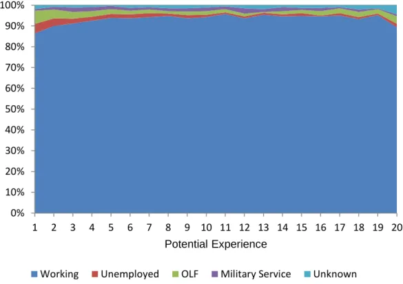
In the NLSY it is possible to identify week-by-week records of individuals' labor force status since 1978. I use these variables to calculate for each potential experience year (age minus schooling minus six) the share of weeks that each worker in the sample spent working, unemployed, out of the labor force, or in active military service. I use this information to present statistics on average employment attachment over the life cycle for high school graduates and workers with at least a college degree in gures 1.1 and 1.2, respectively. These gures reveal that both high school and college graduates spend on average a signicant share of their time after leaving school not working, although career interruptions happen much more often for the former group.

A surprising nding from these gures is that non-black males spend a signicant share of their time out-of-the labor force throughout their careers. Although the NLSY provides limited information on the reasons for non-participation of workers, I did some further in-vestigation of the available data for why these group of workers are out-of-the labor force.13

The results show that the reasons are very diverse, with the three most common reasons being individuals that did not want to work (20%), had a new job they were to start (19%) and were ill or unable to work (14%).

13_{The data is limited due to the changes of questionnaires across years. These statistics are based on the}

(25)

In addition to week-by-week information, NLSY also provides information on weeks between interview years that an individual spent working, unemployed, out of the labor force, or in military service14_{These retrospective variables were used to construct the main work history}

variables used in the paper, as presented in table 1.2. More specically, for each individual, work experience is dened as the cumulative number of weeks spent working since leaving school. In addition, cumulative unemployment, OLF, and military service years were dened as the number of weeks spent in each of these labor force conditions since leaving school. I then divide all variables by 52, so that the measurement unit is year.15 _{Throughout the}

paper, potential experience is dened as age minus schooling minus six. This is the variable typically used in the literature (table 1.1) to measure experience, and as discussed before, it does not distinguish working and non-working periods throughout a worker's career. Note that because some individuals take more time to nish school than their schooling years, potential experience does not accurately measure the years a worker is in the labor market. For this reason, I also use time since leaving school as an alternative measure of experience that does not account for non-working periods. Note that time since leaving school is just the sum of the other cumulative work history variables.16

The wage is calculated as the hourly rate of pay (measured in year 1999 dollars) for the

cur-14_{There is also information on the percentage of weeks that NLSY cannot be accounted for. I use this}

information as a control in all regressions.

15_{In section 1.3.2 I also explore the possibility that timing of career interruptions might aect earnings.} 16_{An issue I faced while creating the work history variables is the fact that 7% of the individuals in the}

sample graduated before 1978 and there is no available information regarding their work history before this year. I try to overcome this problem by using information available on when a worker left school (a year before 1978) and impute the work history variables described in table 1.2 for these individuals, between the year of leaving school and the year 1978. The imputation method consists of calculating the number of work/unemployment/OLF/military service weeks for the 1978 calendar year, and the assumption that it was constant between the year of leaving school and 1978. An alternative approach is to drop the 196 individuals who graduated before 1978 from the analysis. The results of this second approach are quite similar to imputing the work history variable, so I decided to omit them in this paper, but they are available upon request.

(26)

rent or most recent job of a worker.17 _{In order to perform the earnings equation estimation,}

I also restrict the observations to individuals employed at time of interview who work for hourly wages higher than $1 and less $100.18 _{After these sample restrictions given above, the}

remaining sample consists of 2,484 individuals with 33,707 observations. All the statistics in the paper are unweighted.

Table 1.3 contains the main statistics of the sample used in the earnings equation estima-tions for dierent educational levels. This table highlights some important features of the data. First, the mean of the potential experience and time since leaving school variables are signicantly greater than the mean of the work experience for all educational groups. This shows that even for non-black males a group with considerably higher employment attachment potential experience substantially overstates actual experience. However, as expected, the dierence is higher for less educated workers. Second, the individuals in all the educational groups spend more time out of the labor force than unemployed throughout their career. Finally, the work history information reported in the NLSY is quite accurate: for only 0.8% of weeks since leaving school NLSY was not able to dene the labor status of the workers in the sample.

1.3.2 Earnings Dynamics Estimation

There are two main earnings models that are estimated in this paper. The rst model represents the typical earnings equation that has been widely used in the literature, which

17_{The hourly rate of pay is calculated in the NLSY from answers to questions concerning earnings and}

time units for pay. If a respondent reports wages with an hourly time unit, actual responses are reported as the hourly rate of pay. For those reporting a dierent time unit, NLSY uses number of hours usually worked per week to calculate an hourly rate of pay.

18_{There are 41 individuals who do not have any observations during the whole period of analysis with}

(27)

shows how the eect of schooling on wages changes with potential experience (see table 1.1). I refer to this model as the traditional model and dene log-earnings of individual iin time

period t as:

lnwit =α0+α1si+α2(si×pexpit) +g(pexpit) +εit (1.3)

where lnwit is the log of hourly earnings, si is years of schooling and pexpit is the poten-tial experience, dened as age - schooling - six or time since graduation, which do not distinguish working and non-working periods and g(.) is as cubic function.19 The primarily interest of the paper is estimating the parameterα2 which identies how the wage coecient

on schooling changes with potential experience. It is important to note that in previous work (table 1.1) this parameter has been consistently estimated as non-positive; I aim to test whether the same result is found in the sample used in this paper.

In addition to equation 1.3, I also estimate a wage model that fully characterizes the past employment and unemployment history of workers:

lnwit =β0+β1si+β2(si×experit) +β3(si×interrit) +f(experit) +h(interrit) +uit (1.4)

where experit is work experience and interrit is a measure of career interruptions since leaving school. The objects of interest are the parameters β2 and β3, which identify how the

wage coecient on schooling changes with work experience and past non-working periods

19_{Mincer (1974) uses log of annual wages and}_g₍_.₎_{function is dened as a quadratic function. But since}

the seminal paper from Murphy and Welch (1990), the convention is to use log of hourly earnings and dene

(28)

respectively.

When modeling an earnings function that accounts for the work history of individuals, a researcher is confronted with some non-trivial choices. First, there is a question regarding the appropriate way to measure career interruptions. It has been shown that dierent labor force status of individuals during career interruptions might have dierent impact on subsequent wages (Mincer and Ofek, 1982 and Albrecht et al., 1999). For this reason, I will follow the literature and make the distinction between periods of unemployment, time spent out of the labor force, and military service periods.

Second, one can claim that the timing of career interruptions is also important for earnings determination. With respect to this issue, the literature has suggested dierent specications, ranging from the simple accumulation of out-of-work periods since leaving school (Albrecht et al., 1999) to a less parsimonious model, which characterizes the number of weeks out of employment for every year since leaving school (Light and Ureta, 1995). For the main results of the paper I will follow Albrecht et al. (1999) and accumulate periods of unemployment and out-of-work since leaving school. However, in subsection 1.3.2 the analogous results using a less parsimonious model are also presented, where timing of non-working periods is important for earnings.

The nal non-trivial choice is how to dene the functions f(.) and h(.). In order to be consistent with the most recent literature on the earnings equation (Murphy and Welch (1990)), I dene f(.) as a cubic polynomial in the main tables of the paper. By analogy, I will also dene h(.) as cubic polynomial, although the coecients of higher order terms are usually not signicant. Nevertheless, I will also present a less-restricted model, where I estimate both f(.) and h(.) non-parametrically in subsection 1.3.2 and the results are

(29)

Main Results

Throughout the paper I normalize the interactions between schooling and measures of work history variables such that coecient of interactions represent a change in the wage coecient on schooling with 10 years of experience, unemployment, or OLF periods. All the standard errors presented are White/Huber standard errors clustered at the individual level.

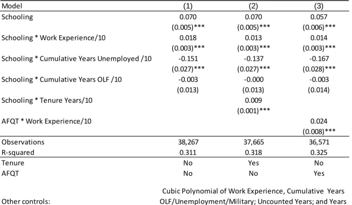
Columns (1) and (2) of table 1.4 show the estimation of the traditional earnings model as presented in equation (1.3). The main point of these estimations is to show that one can replicate the nding of the literature, as presented in table 1.1, using the sample restrictions of this paper. First, in column (1) I estimate that the eect of an extra year of schooling on earnings in the beginning of a worker career is 11% (0.006). Next, I estimate that interac-tion between schooling and potential experience is statistically insignicant. This result is in accordance with Mincer (1974), who found no eects of the interactions between school-ing and potential experience on earnschool-ings (parallel or convergence of log earnschool-ings potential experience proles across educational groups). Finally, in column (2) I estimate the same specication using time since leaving school as a measure of experience. This measure also does not distinguish working in non-working periods but accurately identies the period in which a worker left school. Note that the results from these specications are similar to the ones presented in column (1).

Column (3) provides the estimation of the career interruptions earnings model as presented in equation (1.4). As can be seen, the result from this specication is remarkably dierent from the ones using the traditional model. First, I estimate a lower schooling coecient of 8% (0.005). Second, I nd a positive and signicant coecient of 0.018 for the interaction between schooling and work experience, meaning that the eect of one additional year of

(30)

education increases from 8% to 10%, after a worker accumulates ten years of work experience. Furthermore, I estimate a negative eect of the interaction between past unemployment and schooling. Specically, I estimate that the wage coecient on schooling decreases by 2.1%, following one year of unemployment. Finally, I nd a positive but not signicant interaction between OLF periods and schooling.20 _{But, as discussed in section 1.3.1,}

the interpretation for the impact of OLF periods on wage for this demographic group is challenging due to heterogeneous reasons that lead to this type of career interruption. Columns (4) and (5) provide more robustness to the previous results. In column (4) tenure and its interaction with schooling are added to the model. The idea behind this addition is to investigate whether the main ndings of the paper are due to the period a worker is attached to a particular employer, rather than general labor market experience. From these estimations, I nd that: i) the coecients of the career interruptions model are barely aected by the inclusion of these variables; and ii) the wage coecient on schooling is not signicantly aected by tenure. This result suggests that rm-specic mechanisms are not the main explanation for the empirical ndings of the paper. This is the approach that is followed in section 1.4.

In column (5) Armed Forces Qualication Test score (AFQT) and its interaction with work experience are added to the earnings equation.21 _{The AFQT score has been used in the}

employer learning literature (Farber and Gibbons, 1996 and Altonji and Pierret, 2001) as a measure of a worker's ability that is not easily observed by rms. According to this literature, when AFQT is included with its interaction with experience in the earnings equation, it causes the decreasing with experience (as described in table 1.1). Note that this result is not

20_{I also reject with 99% condence that the coecient of the interaction between schooling and}

unemploy-ment is equal to the coecient of the interaction between OLF periods and schooling.

(31)

found in a model that accounts for career interruptions of workers: while there is a decline of β2 from columns (3) to (5), the coecient is still positive and signicant. In addition,

the other coecients of interest remain practically unchanged with the inclusion of AFQT in the equation.

Figures 1.3, 1.4, and 1.5 illustrate how the wage coecient on schooling changes with the work history variables used in the paper. In these gures I report the coecients of schooling with a 95% condence interval estimated from the same earnings model as presented in column (3) of table 1.4. The only dierence is restricting the sample to workers within a specic range of work history variable (as presented in the x-axis) and the omission of the interaction terms between schooling and work history variables from the equations.

Based on this approach, gure 1.3 shows a wage coecient on schooling of 8% for workers with 0 to 4 years of work experience. However, this coecient rises for workers with higher experience levels. In precise terms, I estimate the eect of schooling on earnings at 11% for workers with 16 to 20 years of work experience. In contrast, gure 1.4 shows that the wage coecient on schooling tends to decrease for workers with higher levels of cumulative unemployment. In fact, I estimate that workers with 0 to 0.4 cumulative years of unem-ployment have a 10% wage coecient on schooling, while workers with cumulative years of unemployment between 1.6 and 2 are rewarded only 4% for an extra year of education. Finally, gure 1.5 shows that the wage coecient on schooling does not change signicantly within OLF groups. All these results are consistent with the ndings of table 1.4.

As discussed in section 1.3.1, the main group of interest for this work is non-black males. Nevertheless, one might be interested on the empirical results for other demographic groups. In table 1.5, I present the results of the career interruption model for black males, non-black females and black females in columns (1), (2) and (3) respectively. The main ndings are

(32)

similar to those for non-black males. For black males and non-black females, I estimate: i) a positive and signicant eect of the interaction between work experience and schooling; and ii) a negative eect of the interaction between past unemployment and schooling on earnings. Neither work experience nor cumulative unemployment have a signicant eect on the returns to schooling for black females. Finally, past OLF periods have a negative impact on the returns to schooling for both non-black and black females. However, it is well-known that reasons for non-participation periods are substantially dierent for males and females, which poses a challenge for comparing the results for these two groups.

Finally, table 1.6 provides robustness check that the main results of the paper are not sensitive to the denition of the year of leaving school. In precise terms, and dierent from the other results of the paper, in this table a worker enters the labor market when he rst leaves school and the accumulation of work, unemployed and OLF weeks start in this period. As discussed before, on one hand, some of the career interruptions can be justied by a decision of a worker to return to school after spending some time in the labor market. On the other hand, I can account for employment periods a worker had before returning to school in the construction of the work experience.

The table shows that the results using this denition for year of leaving school is very similar to the ones presented in table 1.4. In fact, in column (1) I estimate a 7% eect of schooling on earnings at the beginning of a workers career. Second, there is a positive and signicant coecient of interaction between schooling and work experience of 0.018. In contrast, there is a negative eect of the interaction between past unemployment and schooling of 0.151 and insignicant eect of OLF periods on the returns to schooling. In addition, in columns (2) and (3) I nd similar results when including tenure and AFQT and its interactions with schooling and work experience respectively on the wage equation.

(33)

Earnings Proles and Nonparametric Regressions

In this subsection I estimate a less restricted earnings model without imposing functional form assumptions on the relation between work experience, cumulative unemployment, and OLF years and earnings. In these estimations I also substitute years of schooling with educational degree dummies. This procedure allows the model to account for non-linearity in the relation between schooling and earnings. The earnings proles are plotted with respect to work experience, cumulative years unemployed, and cumulative years OLF for dierent educational groups. The estimated non-parametric model is the following:

lnwit=fs(experit) +hs(cunempit) +gs(colfit) +ηit (1.5)

where s represents educational group variables: less than high school, high school degree,

some college and bachelor degree or more. As beforeexperitis work experience. I also dene

cunempitas the cumulative years a work spent unemployed, andcolfitas the cumulative years a worker spent OLF. Dierent from model (1.4), there is no imposition of any parametric restriction on fs(.) , hs(.) and gs(.). However, I still impose the additive separability of the work history variables in the model. The method used for the non-parametric estimation is the dierentiating procedure described in Yatchew (1998).22 _{I use locally weighted regressions}

using a standard tricube weighting function and a bandwidth of 0.5 when estimatingfs and 0.25 when estimating hs and gs.23

Figure 1.6 plots the estimate of fs(.) for dierent educational groups. The gure shows 22_{In this method, I estimate each function} _f

s(.), hs(.), gs(.) separately, imposing a functional form

as-sumption for the non-estimated functions. In precise terms, when estimatingˆgs(.), I assume thatfs(.)and hs(.) are cubic polynomial but impose no parametric restriction on gs(.). The same procedure is applied

when estimating_fsˆ₍_.₎_andˆ_hs₍_.₎_.

(34)

that the log earnings-work experience proles have a concave shape as previously found in the literature (Murphy and Welch, 1992), with wages growing faster at the beginning of a worker's career. In contrast to previous literature, I estimate a much steeper wage growth for more educated workers, than for uneducated workers. In fact, the gure shows that the wage gap between individuals with at least a college degree and other workers tends to increase as workers accumulate actual experience. Similarly, the wage gap between high school graduates and workers with less than a high school education is smaller than it is for workers with zero work experience, but increases signicantly as workers accumulate experience. These results are in accordance with the ndings presented in table 1.4, namely that the wage coecient on earnings increases, as workers accumulate actual experience throughout their careers. Figure 1.7 presents the non-parametric estimation of the relation between log earnings and cumulative years of unemployment, dened by the function hs(.) in equation (1.5), for dif-ferent educational groups. The gure shows that both college and high school graduates are negatively aected by unemployment periods, as wages decline with the accumulation of this variable. However, the rate of wage decline is substantively dierent across educational groups since workers with a bachelor's degree have a greater wage decline with unemploy-ment. It is also notable that the wages of workers with less than a high school degree are not signicantly aected by unemployment.

Finally, gure 1.8 plots the analogous estimation of the relation between log earnings and cumulative years that a worker spends out of the labor force, as described by the function

gs(.). The evidence shows that this relation is quite heterogeneous among the groups. While the earnings of workers with at least a college degree are almost not aected at all by the accumulation of OLF, workers with less than a high school degree face a substantial wage decrease with OLF periods. The interpretation of these results is dicult because

(35)

non-participation periods have heterogeneous justications among workers. Timing of Career Interruptions

This section addresses whether accounting for timing of career interruptions in the earnings equation can aect the main ndings of the paper. For this reason, instead of assuming that wages are aected by the cumulative unemployment and out-of-the-labor-force periods, I estimate the following log wage model separately by educational groups:

lnwit =β0S+β S 1 +fs(experit) + 5 X j=1 γ_jsunempit−j + 5 X j=1 αs_jolfit−j+ηit (1.6)

where s represents educational group variables: less than high school, high school degree,

some college, and bachelor degree or more; unempit−j is the number of weeks a worker spent unemployed in the calendar year that was j years before the interview and olfit−j is the number of weeks a worker spent out of the labor force in the calendar year that was j

years before the interview date. For example, for t =1993, the variable unempit−3 reports

the number of weeks a worker spent unemployed in 1990 and olfit−3 the number of weeks a

worker spent OLF in 1990.24 _{I divide}_unemp

it−j andolfit−j by 52, allowing the coecients to be interpreted as changes of year units. Finally, I limit the sample to observations of a worker 5 years after leaving school, so past work history variables reect events that happened after a worker made the transition to the labor market.

Figure 9 plots the estimation of the coecientsγs

j with a 95% condence interval for dierent

s and j. The graph shows a few interesting facts. First, the weeks spent unemployed in the 24_{These career interruption variables are constructed based on the week-by-week work history information}

provided by NLSY, which identies with precision the periods of unemployment and OLF throughout a worker's career.

(36)

past calendar year have the highest impact on earnings for all education groups, but the eects are much higher for workers with a bachelor's degree or higher. In precise terms, the estimation shows that spending the previous calendar year unemployed decreased the earnings of this group by 60%. Second, unemployment periods have a long-term impact on earnings, with a signicant negative eect of unemployment weeks, which occurred 5 years prior to the interview. While the dierence across educational groups is not as strong, this gure shows that educated workers are also more aected by older unemployment periods. In gure 1.10, the analogous statistics for αs

j are reported with a 95% condence interval, showing that periods spent out of the labor force have a negative impact on the earnings of all workers. However, this eect is much lower than those estimated by unemployment periods, and tend to disappear with time. Finally, while it is estimated that college-graduate workers are more aected by past year OLF weeks than educated workers, the dierences across educational groups are not as strong for OLF periods as they are for unemployment periods.

Figures 1.9 and 1.10 bring to light how unemployment and OLF periods aect the eect of schooling on earnings. In order to provide a more accurate test regarding whether the returns to schooling change throughout a workers' career in a model where timing of career interruptions aect wages I estimate the model below:

lnwit =β0+β1si+β2(si×experit) +f(experit) + 5 X j=1 λjunempit−j (1.7) +P5 j=1πj(si×unempit−j) + P5 j=1ρjolfit−j + P5 j=1ψj(si×olfit−j) +it

(37)

wage coecient on schooling changes with work experience, πj which identies how the wage coecient on schooling changes with past unemployment periods j years before the

interview and ψj which identies how the wage coecient on schooling changes with past OLF periodsj years before the interview.

The result of the estimation of the earnings model 1.7 is presented in table 1.7. While I estimate the model including olfit−j and its interaction with si , for the sake of space these coecients are omitted in the table. The result shows that ψj is not signicant for any

j. As can be seen in the table: rst, the wage coecient on schooling increases with work

experience, even in a model where the timing of career interruption matters, as presented in columns (1) - (3). As can be seen, the estimated β2 is not very dierent from the one

estimated in table 1.4. Second, as column (2) shows, previous unemployment periods have a signicant negative impact on earnings, with previous year unemployment having the highest impact. Third, column (3) shows that, although there is an estimated negative eect of all unemployment periods on the wage coecient on schooling for all years, recent unemployment periods have a higher impact on earnings. The overall interpretation of these ndings is that, while timing of unemployment and OLF might matter for earnings determination, this less-restricted model shows similar patterns, in terms of the eect of work experience and career interruptions on the wage coecient on schooling, as the one presented in subsection 1.3.2.

Individual Fixed-Eects Estimates

An issue that emerged in models that fully characterize an individual's work history is the possible endogeneity problem of actual experience and career interruptions. The main argu-ment is an omitted variable problem. It is possible that there are some variables not observed

(38)

in the data that are related to both current wage determination and past employment. For example, workers with higher career aspirations might have higher employment attachment throughout their life-cycle earnings. In both cases, the seriousness of the endogeneity prob-lem depends on how strong the correlation between current and past levels of the earnings residuals is, and whether past residuals are related to the employment attachment of workers. A popular approach in the literature when dealing with possible endogeneity of work history is based on an individual xed eect assumption (Corcoran and Duncan, 1979, Kim and Polachek, 1994, Light and Ureta, 1995 and Albrecht et al., 1999).25 _{The basic idea of this}

approach is that the factor related to past employment attachment of workers which causes the correlation of earnings residuals across time is an individual-specic xed component. In terms of the model presented in equation 1.4, the xed eect assumption means that

uit can be written as a sum of an individual component φi and a transitory component ηit, both with mean zero and constant variance. Whileηit is independent of an individual's work history, the work history variables can be correlated to φi.

Table 1.8 presents the main results of the estimation of the wage model described by equa-tion (1.4) using an individual xed eect estimaequa-tion. Note that as schooling does not change overtime, I cannot identify β1 when using this estimation strategy. However, it is possible

to identify the eect of its interaction with other time-varying variables, such as work

expe-25_{There are other suggestions in the literature with respect to ways of addressing the possible endogeneity}

of work history. Mincer and Polachek (1974) suggest using family characteristics, such as education of the partner or number of children, as instruments for previous working and non-working periods of married women. While it is questionable as to how exogenous these variables truly are, there is evidence that family characteristics have a weak relation to employment attachment of non-black males, the main group of interest of this work. Alternatively, Altonji and Pierret (2001) suggest using potential experience (pexpit)

as an instrument for actual experience, in a model that earnings are not aected by unemployment periods. However, if career interruptions have impact on wages, the potential experience variable is not a validity instrument for actual experience. In this circumstance, pexpit is not redundant (or ignorable) in the log

(39)

rience, tenure, and cumulative years OLF and unemployment. In order to make these new results comparable to the least square estimation, the same specications are followed in this table as the one presented by the least square estimation of table 1.4.

The overall results from table 1.8 are qualitatively and quantitatively similar to those esti-mated by the least square estimation of table 1.4. Namely, the wage coecient on schooling increases signicantly as a worker accumulates work experience, and decreases as a worker accumulates unemployment periods. If anything, the xed eect estimation shows a lower negative coecient for the eect of unemployment on the returns to schooling. In other words, this new estimation leaves the conclusions based on the OLS regressions intact. This result is not surprising in light of the ndings of existing literature. Mincer and Po-lachek (1974), Blackburn and Neumark (1995), and Albrecht et al. (1999) have found that coecients of the earnings model stay virtually unchanged when dealing with the possible endogeneity problem of work history variables. From these results, one can conclude that the endogeneity of work history appears to be less of a problem when estimating career interruptions models.

1.4 Model

The dynamics estimated thus far are puzzling for conventional models of labor market dy-namics. Unlike the past empirical literature, my research nds that more educated workers have a higher increase in earnings with actual experience, while suering greater earnings losses after unemployment periods. This raises the question as to which economic reasons can explain this relationship. Is it possible to conciliate the existing theories for earnings dynamics with these novel empirical ndings? In order to answer these questions, in this

(40)

section I present an economic model that can rationalize the empirical ndings of this paper.

1.4.1 The model environment

A worker enters the labor market in period 0and lives forT periods. All rms are identical

and the only input used in production is labor. Let yit denote a worker's log-productivity in the t-th period after leaving school.

yit =θig(si, xit) (1.8)

In this specication, θi is the worker's ability, g(si, xit) is a worker's human capital, which is a function of the worker's schooling level si and work experience xit. For exposition, I will omit x and s subscripts henceforth. I assume that both θi and g(s, x) are positive, and ∂g(s, x)/∂s > 0, ∂g(s, x)/∂x > 0 and ∂g(s, x)/∂x∂s = 0. The important assumption is that ability and human capital are complementary in determining the log-productivity, which is captured in the multiplicative specication of (1.8).26 _{An interpretation of the}

complementary assumption is that high ability workers can more eectively use their human capital at work and therefore have higher returns to schooling and experience.27

Furthermore, there are only two types of workers: high ability θH or low ability θL. While schooling and work experience are observed, ability is not observed by either employers or workers. All agents have to make their predictions about a worker's ability based on the information available at each period.

26_{Note that this assumption makes the model dierent from the studies presented in table 1.1.}

27_{Papers making similar assumptions include: Acemoglu and Pischke (1998), Gibbons and Waldman}

(41)

Information structure

The only available information regarding ability in period 0 is a worker's schooling level s.

I dene ps as the fraction of workers with schooling level s that are high ability. I assume that ps is dierent from zero and one, and it is strictly increasing with a workers schooling level, meaning that high ability workers are more likely to get more education. Note that in this version of the model, I do not model schooling decision of workers, but this assumption is consist with the signaling literature (Spence, 1973) where high ability workers have lower costs to acquire education. Nevertheless, later I sketch how the model could be enriched to allow for the endogeneity of schooling.

In addition to schooling, I assume that in every period some new information about a worker's quality becomes available to all rms.28 _{This new information can be summarized by the}

signal y˜it, which can be a good or bad signal, with high ability workers producing a good signal with probability γH and low ability workers producing a good signal with probability

γL, such that γH > γL. As in Altonji and Pierret (2001), rms will use information on the worker's signals during the past x−1 employed periods to infer a worker's unobservable ability. I dene Iit={y˜i1, ...,y˜ix−1} as the set of observed past signals.

Dierent from Altonji and Pierret (2001), an individual can be in one of two possible states at each period of his career: working or not working. Firms can also observe the employ-ment history of an individual, which is characterized by the number of periods an individual was employed x−1 (work experience minus one) and the number of periods a worker was unemployed u since leaving school (career interruptions).29 As will be claried later, em-28_{This information consists on past on-the-job performance, new letters of recommendation, interviews,}

etc.

29_{Note that by denition}_x₊_u₌_t_{. Given the perfect linear combination between work experience, career}

(42)

ployment history gives extra information about a worker's ability and the timing of working and non-working periods will not be important in the equilibrium of this simplied model.30

Timing and actions

At the beginning of each period the sequence of events and actions are as follows:

1. A fraction δ of individuals are unable to work. These are the workers that are moving

for personal reasons or are not able to be matched to any employer.

2. The other fraction (1−δ) of workers are able to work and draw a new signal y˜it for the period.

3. The employers make job oers based on information available in the period and the new signal y˜it.

4. A worker can either:

• Choose to work in the period. In this case, a worker accumulates one period of work experience and keeps the signal for future wage oers.

• Choose to not work in the period. In this case a worker accumulates one period of unemployment, while discarding the signal that will not be used for future wage oers.

any of the three variables. For expositional purposes, I choose to present it as work experience and career interruptions. I also ignore the dierence between unemployment and out-of-the-labor-force periods.

30_{This mechanism is consistent with papers where employers use lay o information (Gibbons and Katz,}

1991) or the duration of an unemployment spell (Lockwood, 1991 and Kroft et al., 2013) to infer a worker's unobservable quality. However, in this paper rms take into consideration the full work history of an individual.

(43)

Note that in the model unemployment can be involuntary or voluntary. Involuntary unem-ployment is caused by a worker who could not be matched to any employer in a given period (fractionδ), while voluntary unemployment results from a worker's decision to reject any job

oer. I assume that rms cannot distinguish between these two types of career interruptions when making future wage oers. The idea is that (low performance) workers can always tell the employers that they did not work in a period because exogenous reasons were preventing them from working. Nevertheless, rms pay close attention to the accumulation of career interruptions, and workers are unlikely be able to justify the long periods of unemployment as involuntary.

Firms' decision

Firms do not discount the future and long term contracts are not allowed. As in Farber and Gibbons (1996) and Altonji and Pierret (2001), I assume that there is free entry of rms and all employers share the same information about a worker's productivity. As a consequence from competition among employers, the wage oered to a workeriin periodtis equal to the

expected productivity given the information available at the period and the new signaly˜it:31

Wit=E[expyit|x, u, s, Iit,y˜it] (1.9)

An alternative representation of the wage set up is to deneµ(s, x, u, Iit,y˜it)as the employers' belief that a worker is high-type based on the information available up to that point. In this framework, I use equation (1.8) to show that the wage level of a worker in period t can be

represented by:

(44)

Wit=µ(s, x, u, s, Iit,y˜it) expg(s,x)θH+[1−µ(s, x, u, Iit,y˜it)] expg(s,x)θL (1.10)

The wage process presented in equation 1.10 shows the two dierent roles of work experience

xin the model. On one hand, the termg(s, x)represents the productivity increase of a worker as he accumulates work experience. This mechanism is dened as the human capital eect of working on earnings. On the other hand, accumulating employment periods also provides information about a worker's type, which is represented by the term µ(s, x, u, Iit,y˜it). This mechanism is referred to as the information eect of working on earnings. Furthermore, rms will also use information regarding career interruptionsuin the assessment of a worker's type.

Worker's decision

I assume that workers are risk neutral and discount the future using a discount rate β >0. At each period a worker has access to the same information as rms.32 _{In this framework,}

for individuals that are not exogenously unable to work, the work decision in the rst T −1 periods of their career is dened by the following Bellman equation:33

V(s, x, u, Iit,y˜it) = max{Wit(s, x, u, Iit,y˜it) +β(1−δ)E[V(s, x+ 1, u, Iit,y˜it,y˜t+1)],

b+β(1−δ)_E[V(s, x, u+ 1, Iit,y˜t+1)] (1.11) 32_{As it would be clear in equilibrium, even if workers have better information regarding their own ability}

than rms, this information will be irrelevant for their working decisions.

(45)

where b is the utility ow for not-working. This Bellman equation highlights a trade-o

associated with the employment decision.34 _{On one hand, an individual can choose to work,}

be paid, and accumulate one year of experience. In this case, the signaly˜it is used for current and future wages oers. On the other hand, a worker could discard the signal, receive non-working benets and accumulate one period of unemployment. In this case, rms will not be able to distinguish whether the unemployment period was due to a worker's choice or to an exogenous reason. Nevertheless, rms will use the extra non-working period information to update their beliefs about a worker's ability, and this unemployment information will be used for future wage oers.

1.4.2 Equilibrium

Equilibrium is characterized by a function of the state variablesSit ={s, x, u, Iit}and signal ˜

yit to the rms' belief that a workers is high type µit, a wage oer Wit and an individual's decision to work in period t. From this general framework, it is possible to derive some

predictions of an individual's optimal working strategy and how rms use past employment and unemployment information to update their beliefs about a worker's type.

Proposition 1: For a given stateSit, if it is an optimal strategy for an individual to choose to work after a bad signal draw, it is also an optimal strategy to work in case of a good ability draw.

The justication is straightforward: the rms' belief that a worker is high type is greater after a good signal revelation than after a bad signal. As a result, present and future wage

34_{Note that individuals are exogenously unable to work in period}_t_{+ 1}_{with probability}_δ_{. As the utility}

from this state is independent of previous work choices, this possibility should not aect an individual's decision to work in periodt. In precise terms, the future expected utility of being exogenously unemployed

(46)

oers must be higher after a good signal than after a bad signal. For this reason, for any given state, a worker is better o taking the job after a good signal draw than he would be working after a bad signal draw.

This proposition has implications for the adverse selection and employer learning mechanism proposed by the model. Firms realize that workers with bad signals are more likely to be un-employed and workers with good signals are more likely to be un-employed. Even though rms cannot observe signals produced in the non-working periods, or ascertain whether unemploy-ment was caused by an exogenous reason, they use information on career interruptions and employment periods to update their beliefs about a worker's ability.

Separating Equilibrium

The analysis is now restricted to a separating equilibrium where for any given state, indi-viduals always choose to work after observing a good signal draw, and always decide to not work after observing a bad signal draw. This extreme case highlights the mechanisms of adverse selection and employer learning through work history that I want to stress with the model. It also simplies the calculation of rms' beliefs and wage oers, and the derivations of the predictions of the model.

Some extra assumptions are required in order to guarantee the existence of such a separating equilibrium. First, I assume that high-ability workers always produce a good signal, such that γH = 1, while low-ability workers can produce both good and bad signals: 0< γL <1. The direct implication of this assumption is that the decision to work after a bad signal is sucient to reveal to employers that a worker is low type for the rest of his career.

(47)

ability. For this reason, I assume the productivity of a low ability worker is always lower than his non-working utility, such that expg(H,T)θL _{< b}, where _H is the highest schooling level a worker can achieve and thereforeg(H, T)is the highest human capital level a worker can possibly have. An interpretation of this assumption is that low-ability jobs are so much less rewarding, that workers would never reveal to rms that they are low ability.

Finally, for any stateSit, it must be optimal for an individual to choose to work after a good signal. For this reason I impose the following restriction on θH:

e

µexpg(0,0)θH₊₍₁₋

e

µ) expg(0,0)θL _{> b} (1.12) whereg(0,0)is the lowest human capital level an individual can possibility have (zero school-ing and zero actual experience) and µe represents the lowest believe a rm can have that a

worker is high type in this separating equilibrium. This term is a function of the parameters

ps, δ, and γL and T, and is derived in the appendix of the paper. An interpretation of this assumption is that high-performance jobs are very rewarding and an individual would always work after a good signal.

Under these assumptions, for any state Sit the optimal choice of an individual, that is not exogenously unable to work, is to be employed if y˜it is a good signal and to be unemployed if it is a bad signal. Note that the set of signals Iit becomes trivial, since individuals only work in good signal periods. In this case, the setIit is equivalent to the employment periods

x and therefore will be omitted henceforth.

Within this framework, it is easy to derive the fraction of workers that are employed and unemployed at each period, and the rms' equilibrium belief that a worker is high type. First, the fraction of high-ability individuals that are employed in each period is equal to