Department of Economics
Working Paper No. 186
The Gender Wealth Gap in Europe
Alyssa Schneebaum
Miriam Rehm
Katharina Mader
Patricia Klopf
Katarina Hollan
October 2014
The Gender Wealth Gap in Europe
Alyssa Schneebaum∗ Miriam Rehm†
Katharina Mader‡ Patricia Klopf§
Katarina Hollan¶
Abstract
This paper studies the gender wealth gap using 2010 Household Finance and Con-sumption Survey data for 15 European countries, and finds that households with only one male adult have more net wealth than households with one female adult, and that households with an adult couple have the highest net wealth. Using OLS regressions to predict net wealth and the inverse hyperbolic sine transformation of net wealth, as well as the nonparametric DiNardo-Fortin-Lemieux re-weighting technique, to study the relationship between household and personal characteristics with net wealth, the paper finds that differences in labor market characteristics between male and female households, most notably lifetime labor force participation and wages, explain much of the gender wealth gap.
JEL Classifications: D31; J16; E21
Key Words: Gender; Wealth; Wealth Gap; Distribution
∗
Department of Economics, Vienna University of Economics and Business (WU). Address: Welthandel-splatz 1, 1020 Vienna (Austria). Email: alyssa.schneebaum@wu.ac.at
†
Department of Economics and Statistics, The Vienna Chamber of Labour (AK Wien). Address: Prinz Eugenstraße 20-22, 1040 Vienna (Austria). Email: miriam.rehm@akwien.at
‡
Department of Economics, Vienna University of Economics and Business (WU). Address: Welthandel-splatz 1, 1020 Vienna (Austria). Email: katharina.mader@wu.ac.at
§
Department of Global Business and Trade, Vienna University of Economics and Business (WU). Ad-dress: Welthandelsplatz 1, 1020 Vienna (Austria). Email: patricia.klopf@wu.ac.at
¶
Austrian Institute of Economic Research (WIFO). Address: Arsenal, Objekt 20, 1030 Vienna (Austria). Email: katarina.hollan@wifo.ac.at
1
Introduction
Questions surrounding the distribution of wealth have recently witnessed a surge in interest, which has been closely related to the availability of high quality micro data. Much of the existing literature on wealth distributions focuses on the United States and the United Kingdom (e.g. Wolff, 1998), with more limited research on European countries (e.g. Frick et al., 2010; Bover, 2010; Piketty, 2014). Deepening the investigation into wealth differences between socioeconomic groups, for instance by race (Oliver and Shapiro, 1997), has also been focused on regions for which data are available. Thus far, gender has not been a prominent topic in this research, despite some notable exceptions (e.g. Deere and Doss, 2006a; Yamokoski and Keister, 2006; Sierminska et al., 2010). Especially in contrast to the gender pay gap, a favorite topic among labor economists and sociologists, the gender wealth gap has received far less attention in the literature. Reasons have been the relative shortage of wealth data compared to income data, and the difficulty in untangling ownership information (Sierminska, 2014).
This paper presents an analysis of the gender differences in wealth for the euro area based on a survey harmonized by the European Central Bank, the Household Finance and Consumption Survey (HFCS). The HFCS contains household-level information on net wealth, defined as real plus financial assets minus debt. Detailed socioeconomic data on the household and its members allow researchers to compare households with similar characteristics to test the role of gender in determining a household’s wealth.
The HFCS enables researchers to take large strides in studying the distribution of wealth by gender by providing harmonized data for most euro area countries, but the HFCS data are aggregated on the household level. Having data on the wealth of households, not individuals, complicates the analysis of the intra-household distribution of wealth, particularly because household members may not have equal access to wealth (Grabka et al., 2013; Sierminska et al., 2010) or decision-making power (Mader and Schneebaum, 2013). This paper goes around this problem by restricting the analysis to three groups: households headed by male reference persons with no partner living in the household (male single households, or just “male households”), households headed by female reference persons with no partner living in the household (female single households, or just “female households”), and households whose reference person is a member of a different-sex couple, where the spouse or partner is living in the same household.
The paper investigates the difference in wealth between couple households, male house-holds, and female households by using three multivariate econometric methods. First, for compatibility with the existing literature, OLS regressions predicting the level of house-hold net wealth are performed using a vector of standard and novel explanatory variables. Second, to account for the highly right-skewed distribution of net wealth, the regression is also done using an inverse hyperbolic sine (IHS) transformation of the net wealth data. Third, since the gender wealth gap varies over the unconditional net wealth distribution, a nonparametric decomposition developed in Fortin et al. (2010) (DFL) is used to study
the correlation of various characteristics with the gender wealth gap across the entire distribution of net wealth.
The results are in line with the existing literature on gender differences in the wealth distribution in the US, UK, and Germany, and also with the much more established lit-erature on the gender wage gap (e.g. Blau and Kahn, 1997; 2000; Weichselbaumer and Winter-Ebmer, 2005; Plantenga and Remery, 2006). Labor market characteristics go a long way towards explaining the differences in wealth between male and female households, even though a gap in wealth based on households type remains even after all measurable characteristics are controlled for. Male households have higher wealth than female house-holds, which is largely due to differences at high levels of net wealth – the equivalent of a “wealth glass ceiling.” The contributions of this paper are the estimation of the gender wealth gap for the entire euro area, and the application of DFL decomposition to study the gender wealth gap across the entire distribution of net wealth.
The paper is structured as follows: Section 2 gives an overview of the theoretical and empirical background of gender differences in the accumulation and distribution of wealth, Section 3 presents the data and methods, and Section 4 contains the empirical results. Section 5 concludes.
2
Gender Differences in Wealth Accumulation
As discussed in Wolff (1998), there are various reasons why people own different levels of wealth: they are at different stages in the life-cycle; levels of entrepreneurial spirit as well as success differ; they have distinct tastes for income, human capital accumulation, and savings; and luck is unevenly distributed across the population. Despite the fact that we already know quite a bit about how wealth is accumulated, studies on inequality in wealth distribution have often neglected the issue of gender (e.g. Wolff, 1998). There are, however, good reasons to expect that wealth is unevenly distributed by gender. Consider the following simple model of wealth accumulation, taken from Schmidt and Sevak (2006, p.142):
At+1 = (1 +rt)(At+Yt−Ct). (1)
The model in equation 1 says that a household’s stock of wealth or assets A in time
periodt+ 1 is a function of the stock of assets (At), the income earned (Yt), along with
the consumption level (Ct) in a previous time period t, and the rate of return on those
previously accumulated assets,rt. Inheritances and other wealth transfers can increase or
decrease the stock of assets given byAt. The rate of returnrt depends on risk preferences
and portfolio selection. Assume that the rate of return on investments is constant across periods. What determines these components of wealth, and how might they differ by gender?
Higher levels of schooling are consistently shown to be positively related to greater income
(see e.g. Card, 1999). Greater income allows for more saving (Yt−Ct in equation 1),
increasing wealth, meaning that more educated people should have more wealth. There are other channels beyond income through which education influences wealth, as well. A higher level of education can lead to more knowledge of investment opportunities
(affect-ing rt in equation 1). Also, given intergenerational persistence in educational outcomes,
more highly educated people are likely to have highly educated parents (Hertz et al., 2007; Schneebaum et al., 2014). Those parents will likely have higher income and wealth them-selves, leaving them with valuable assets to pass to their children in inheritances later.
These inheritances affect a person’s wealth by increasingAt. Since educational outcomes
differ by gender, women are at an educational wealth disadvantage. Women had lower levels of educational attainment on average until only recently (and still do in some coun-tries) (see e.g. Schneebaum et al., 2014), we can therefore expect women to accumulate lower levels of wealth than men.
Wealth can also vary over the life-cycle, an observation described by the life-cycle hy-pothesis (Modigliani, 1966). This hyhy-pothesis states that individuals seek to smooth their consumption over time to maintain a constant lifestyle, and will make their consumption and saving decisions accordingly. Individuals will thus save part of their income during their working years in order to afford comparable consumption in retirement. However, a high rate of dis-saving in retirement implied by the life-cycle hypothesis is not unam-biguously observed in the empirical literature (e.g. Piketty et al. (2011)). Nevertheless, wealth over age broadly tends to have an inverted u-shape form. Since women typically live longer than men, we may therefore expect higher levels of wealth for women based on age. Further, women are more likely to outlive their husbands than the other way around, so women will be more likely to inherit from their husbands, contributing to their wealth in old age.
Labor market characteristics are also important determinants of wealth, and income and wealth are highly positively correlated (Piketty and Zucman, 2014). In equation 1
in-come affects wealth through savings,Yt−Ct. Women on average receive lower wages than
men for the same work (Blau and Duncan, 1967; Council of the European Union, 2010), and women are more likely to work in part-time jobs as a result of care and housework responsibilities, which are still primarily assigned to women (Jepsen et al., 2005; Manning and Petrongolo, 2007; Bardasi and Gornick, 2008; Fernández-Kranz and Rodríguez-Planas, 2009; Matteazzi et al., 2012). Relatedly, women are more likely to face interruptions in their working histories, further shortening the time spent in the labor market (Budig and England, 2001; Gangl and Ziefle, 2009). The disadvantages women face in the labor market, namely lower income levels and shorter paid working time, result in weaker pos-sibilities for women to accumulate wealth. Women have to work longer to earn the same amount of income as their male counterparts and therefore also need to work more to ac-cumulate comparable levels of wealth, holding the saving rate and other factors constant across gender.
Inheritances are an important part of wealth accumulation and contribute directly
toAt in equation 1. Some empirical papers find that inheritances comprise around half
of households’ wealth (Gale and Scholz, 1994); the rest is formed by savings and other
transfers. Other studies find support for the so-called law of 20/80, which states that
inheritances constitute up to 80% of household wealth (Kotlikoff and Summers, 1988). Still others find the exact opposite to be true, namely that only around 20% of total wealth are inherited and the rest accumulated through saving (Modigliani, 1988). Some of the variation in findings on the role of inheritances in determining net wealth arise from differences in conceptualizations of inheritances: it is unclear whether inter vivo transfers, such as parents’ contributions to the human capital accumulation of their children, for example, should be considered bequests (Deere and Doss, 2006a). There is ongoing debate on the effect of inheritances on the overall level of wealth and wealth inequality (see e.g. Bowles and Gintis, 2002; Piketty et al., 2011; Fessler and Schürz, 2013). Although inheritance regimes differ around the world (see e.g. Deere and Doss, 2006b), there is a clear trend towards equality between genders regarding outcomes of inheritance practices in the countries studied here (Pestieau, 2002). Women may be more likely to inherit because they live longer than men on average, but the value of their inheritances may be lower than men’s (Mader et al., 2014).
Finally, differences in asset allocation patterns and risk preferences, which affect the
rate of return on assets (captured byrtin equation 1), form another cause of wealth gaps.
Decisions concerning asset allocation may differ by gender because of differences in how men and women are socialized (Chang, 2010). It is a widely held belief that women are more risk averse than men, but Nelson (2012) puts together a convincing study which draws this idea into serious doubt. In any case, Neelakantan and Chang (2010) show that an unexplained gender wealth gap persists even once controlling for differences in risk preferences between men and women. Furthermore, having accumulated less wealth due labor market differences and lower educational attainment, women have fewer financial means at their disposal to invest in some more expensive and potentially more lucrative assets, such as stocks, real estate or business assets. Since women own fewer of these high-return assets, they have fewer possibilities to accumulate the same levels of wealth as men.
Empirically, the literature contains unanimous evidence of a gender wealth gap, in which women accumulate less wealth than men. Chang (2010) wrote a book exploring the gender wealth gap, providing an important introduction to and overview of the topic of wealth differences by gender. Chang focuses her analysis on the United States, and uses empirical data from the 2004 Survey of Consumer Finances (SCF) to show that the
gender wealth gap is largely attributable to differences in access to thewealth escalator.1
Chang concludes that “a woman’s wealth gap would continue to exist even if men and women had the same incomes because women are more likely to have custody of children
1The wealth escalator is defined as a set of “legal, institutional and societal mechanisms that help some
and of the expenses that children accrue” (Chang, 2010, p.74). Chang (2010) argues that, based on the theory and empirical findings in the book, a gender wealth gap will continue to exist until social policies, employers, and society erase the economic disadvantages of motherhood.
Many of the empirical studies on the gender wealth gap can be found in a special
issue of Feminist Economics dedicated to differences in wealth by gender (Strassmann,
ed, 2006). A paper by Deere and Doss (2006a) gives a broad overview of studies on the gendered distribution of wealth and summarizes the evidence of a gender asset gap based on historical data from probate records going back to the 19th century. Deere and Doss (2006a) further update this information (using mainly US and UK data), finding a large gender wealth gap which has persisted over time. Other studies included in this issue using more recent survey data are Schmidt and Sevak (2006), Yamokoski and Keister (2006), and Warren (2006). These works look at the wealth holdings of women and men in the United States and the United Kingdom. Schmidt and Sevak (2006) use wealth supplement data from the Panel Study of Income Dynamics (PSID) from 2001 to analyze the differences in household wealth by gender and marital status. They find the largest gap in wealth holdings between married couples and female households, but show that the gender wealth gap almost disappears in a subsample of young households. Yamokoski and Keister (2006) look at the gender wealth gap in the young baby boomer cohort in the USA, using data from the National Longitudinal Survey of Youth (NLSY-79) between 1979 and 2000 and find a large gap between never-married or divorced females and males and married couples, where females have the lowest net wealth. Both single mothers and fathers have lower median wealth than adults without children, yet never-married or divorced single mothers suffer the highest wealth disadvantages (Yamokoski and Keister, 2006, p.189). Warren (2006) analyzes the gender wealth gap in the UK with data from the Family Resources Survey (FRS) of 1996, finding that only 66% of women in the sample owned pension savings while all men did (Warren, 2006, p. 213).
A handful of other studies on the gender wealth gap have emerged in the literature since then. Neelakantan and Chang (2010) analyze the gender wealth gap at retirement using data from the 2006 Health and Retirement Study (HRS) in the United States and find a negative correlation between risk aversion and one’s level of wealth. They show that if women had men’s risk preferences the gender wage gap would decline, but not disappear. Another study exploring wealth differences by gender at retirement was carried out by Denton and Boos (2007). The authors use a sample of respondents older than 44 from the 1999 Canadian Survey of Financial Security and find that women accumulate a third less wealth on average than men. A recent study by Ruel and Hauser (2013) uses data from the Wisconsin Longitudinal Study on 6,821 high school graduates from 1957 to show that variables on status attainment (such as currently working full-time or part-time, being self-employed or retired) had the most power in explaining gender wealth gaps. However, even controlling for gender differences in status attainment, human-capital, investment strategies, family formation, and family-of-origin influences, a gender wealth gap persists.
The studies discussed so far use survey data on wealth that were collected at the household level. The German Socio-Economic Panel (SOEP) survey, however, collects data and reports on wealth at the individual level. Grabka et al. (2013) analyze the intra-partnership wealth gap using this data from 2007. They find a mean gender wealth
gap ofe33,000 in their sample of 7,200 cohabiting couples (regardless of marital status).
In Sierminska et al. (2010), the same authors find that the gender wealth gap within
married couples is aboute50,000, which is largely explained by differences in labor market
participation of husbands and wives. Comparable studies analyzing the gender wage gap at the person level are missing from other countries, where only household level data are available. Sierminska et al. (2010) and Grabka et al. (2013) present evidence that any gender wealth gap between female and male single households may also exist between men and women within a couple.
In our empirical analysis, in which we can only analyze household level data, we expect to find a greater level of wealth in male households compared to female households, which will diminish as we compare male and female households with a similar number of and ages of children, inheritances, and labor market characteristics, and comparable educa-tion, age, and marital status of the respondent. It is unclear how strong the relationship between inheritances and wealth is, and whether men or women will benefit from bequests more. Further, since being older has been associated with higher wealth, we expect female households to benefit from their age structure. However, we expect that some female household characteristics, namely that more female households have children, and that they have lower levels of education and weaker labor market outcomes, will be negatively related to wealth. In the following sections we describe the data and analytical methods we use to test these hypotheses.
3
Data and Methods
3.1 Data
To test for differences in wealth between male and female households data from the 2010 Household Finance and Consumption Survey (HFCS) are employed. The HFCS is a
harmonized survey in all euro area countries.2 Available data of the first wave 20103 are
used. The net sample size is 62,558. The HFCS data provide multiply imputed values for item non-response, which are taken into account in the estimates reported by using Rubin’s Rule.
The HFCS contains detailed information on household net wealth and its components, as well as socioeconomic characteristics of household members, which allow us to include a standard set of controls in tests of the gender wealth gap (Yamokoski and Keister, 2006; Sierminska et al., 2010; Grabka et al., 2013). At the household level, net wealth, earnings,
2Ireland and Estonia did not participate in the first wave of the survey, and Latvia was not yet part of
the Eurozone.
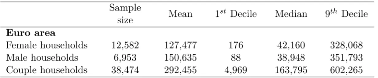
Table 1: Net wealth by household type (ine) Sample
size Mean 1
st Decile Median 9th Decile
Euro area
Female households 12,582 127,477 176 42,160 328,068
Male households 6,953 150,635 88 38,948 351,793
Couple households 38,474 292,455 4,969 163,795 602,265
Source: own calculations using data from 2010 HFCS.
inheritances, and the sector of businesses owned by the household are of particular interest. At the person level, the reference person’s age, gender, education, relationship status, presence of children, and employment status are used.
Like most wealth surveys, the HFCS collects wealth data on the household level. This paper therefore compares three different household types: male households, female house-holds, and couple househouse-holds, as defined in section 1. In order to keep the population under comparison as uniform as possible, the sample of single households is restricted to house-holds whose reference person is living either alone, with children, or with grandchildren. Similarly, only couple households without other adults present are kept. No households in which other adults are present, such as those with the parent of the reference person in the home, are part of this analysis.
The sample thus contains 54,433 households. Table 1 gives an overview of the dis-tribution of net wealth by household type. On average, couple households own roughly
e292,000, male single households hold slightly more than half of that (e151,000), and
female single households have less than half of that(e127,000). While the distribution is
right-skewed for all household types, this is most pronounced for male single households as evidenced by the mean/median ratio.
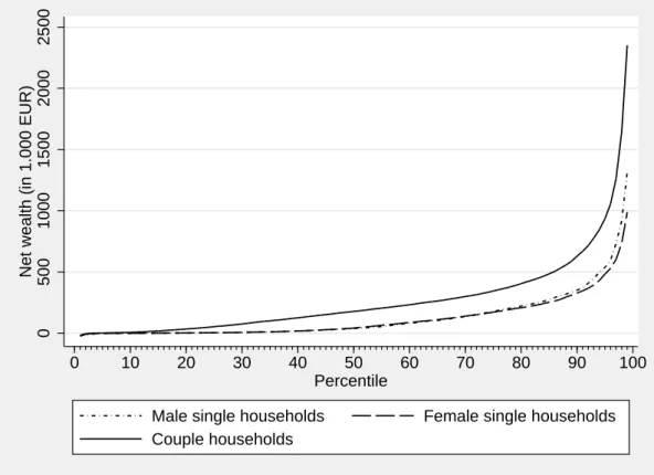
Figure 1 shows this information in more detail. While both male and female single households own less net wealth than couple households, the difference between male and female single households only becomes visible to the naked eye in the top percentiles of the respective household types. At the median, there is not much of a gender wealth gap
- indeed female households at the middle of the distribution havemore wealth then male
households. On average over the entire distribution, though, male household have 15% more wealth.
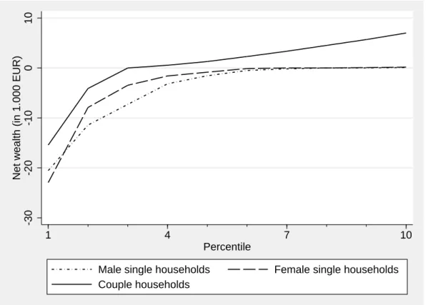
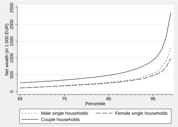
Figures 2 and 3 expand the bottom 10 and top 35 percentiles to allow for a closer look at the distribution of net wealth. The richest male households have more wealth than the richest female households, but male household are also more likely to be indebted (have negative wealth - see figure 2).
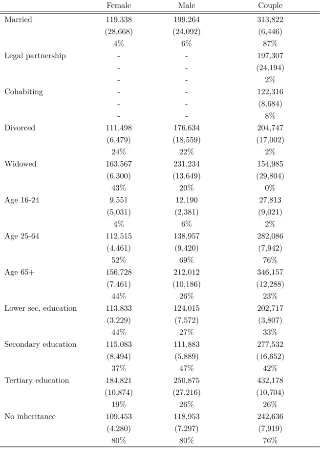
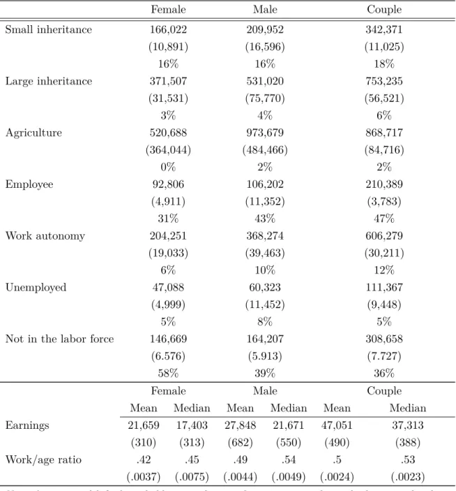
As we describe in the next section, we compare the wealth of male, female, and couple households with similar characteristics to test for a gender wealth gap. Table 2 shows the average of net wealth for households with each variable, along with the share of households in that household type with that characteristic.
0 500 1000 1500 2000 2500
Net wealth (in 1.000 EUR)
0 10 20 30 40 50 60 70 80 90 100
Percentile
Male single households Female single households Couple households
Figure 1: Distribution of net wealth by household type
Source: own calculations using data from 2010 HFCS.
Table 2: Average wealth and proportion of population of variables
Female Male Couple
No kids 129,767 141,476 302,835 (5,484) (7,166) (10,575) 73% 90% 49% Kids≤6 57,383 176,244 181,428 (9,128) (72,811) (6,415) 5% 1% 16% Kids > 6 and≤ 16 86,554 215,807 280,687 (6,338) (51,966) (15,385) 11% 3% 23% Kids > 16 157,461 288,070 351,084 (10,365) (52,399) (10,732) 17% 7% 25% Never married 90,100 105,721 -(6,425) (8,022) -30% 53%
Table 2: continued
Female Male Couple
Married 119,338 199,264 313,822 (28,668) (24,092) (6,446) 4% 6% 87% Legal partnership - - 197,307 - - (24,194) - - 2% Cohabiting - - 122,316 - - (8,684) - - 8% Divorced 111,498 176,634 204,747 (6,479) (18,559) (17,002) 24% 22% 2% Widowed 163,567 231,234 154,985 (6,300) (13,649) (29,804) 43% 20% 0% Age 16-24 9,551 12,190 27,813 (5,031) (2,381) (9,021) 4% 6% 2% Age 25-64 112,515 138,957 282,086 (4,461) (9,420) (7,942) 52% 69% 76% Age 65+ 156,728 212,012 346,157 (7,461) (10,186) (12,288) 44% 26% 23%
Lower sec, education 113,833 124,015 202,717
(3,229) (7,572) (3,807) 44% 27% 33% Secondary education 115,083 111,883 277,532 (8,494) (5,889) (16,652) 37% 47% 42% Tertiary education 184,821 250,875 432,178 (10,874) (27,216) (10,704) 19% 26% 26% No inheritance 109,453 118,953 242,636 (4,280) (7,297) (7,919) 80% 80% 76%
Table 2: continued
Female Male Couple
Small inheritance 166,022 209,952 342,371 (10,891) (16,596) (11,025) 16% 16% 18% Large inheritance 371,507 531,020 753,235 (31,531) (75,770) (56,521) 3% 4% 6% Agriculture 520,688 973,679 868,717 (364,044) (484,466) (84,716) 0% 2% 2% Employee 92,806 106,202 210,389 (4,911) (11,352) (3,783) 31% 43% 47% Work autonomy 204,251 368,274 606,279 (19,033) (39,463) (30,211) 6% 10% 12% Unemployed 47,088 60,323 111,367 (4,999) (11,452) (9,448) 5% 8% 5%
Not in the labor force 146,669 164,207 308,658
(6.576) (5.913) (7.727)
58% 39% 36%
Female Male Couple
Mean Median Mean Median Mean Median
Earnings 21,659 17,403 27,848 21,671 47,051 37,313
(310) (313) (682) (550) (490) (388)
Work/age ratio .42 .45 .49 .54 .5 .53
(.0037) (.0075) (.0044) (.0049) (.0024) (.0023)
Note: Average wealth for household type with given characteristic, with standard errors in brackets and percentage of household type with given characteristic.
Source: own calculations using data from 2010 HFCS.
3.2 Analytical Methods
Three multivariate econometric analyses are performed to identify the gender wealth gap in Europe. First, for comparison with much of the existing literature on the gender wealth gap, Ordinary Least Squares (OLS) regressions predicting the level of household net wealth, controlling for household type and a vector of explanatory variables, are employed.
Net wealth Wi for each household i is regressed on a constant, household type dummy
-30
-20
-10
0
10
Net wealth (in 1.000 EUR)
1 4 7 10
Percentile
Male single households Female single households Couple households
Figure 2: Bottom decile of the distribution of net wealth by household type
Source: own calculations using data from 2010 HFCS.
Wi =β0+β1F emalei+β2M alei+γikXik+δijZij+εi (2)
The main control group of interest is couple households, whose wealth is compared to male and female single households’ (abbreviated “male” and “female” in equation 2 above)
wealth. Fixed effects δij for a household being in country j are included in all models.
Thekhousehold characteristics inX are put into four main groups: household structure;
age and education of the respondent; inheritances; and labor market characteristics of the respondent and household. We add these controls sequentially to test their relationship to the gender wealth gap.
Control set 1, composed of the household structure variables, contains information on the presence of any child(ren) less than or exactly six years old, between the ages of seven and 16, inclusive, or above 16, and whether the respondent is divorced, widowed, never married, in a legal partnership (but not married), or cohabiting without legal recognition of the relationship, via dummy variables. The control groups are having no children in the household and being married. Note that the female and male “single” households used in this study can be in any of the marital status groupings, because the “single” households are identified only by the lack of presence of a partner living in the household, independent of the respondent’s marital status.
0 500 1000 1500 2000 2500
Net wealth (in 1.000 EUR)
65 75 85 95
Percentile
Male single households Female single households Couple households
Figure 3: Top percentiles of the distribution of net wealth by household type
Source: own calculations using data from 2010 HFCS.
respondent. Age is captured in three dummy variables: ages 16-24; 25-64; and 65+, where the middle group is the control. Education is coded by ISCED-97 and is also represented in three categories, where the lowest (only primary or lower secondary schooling completed) is excluded.
A household’s inheritances are controlled for in set 3. Inheritances are notoriously under-reported in wealth surveys (Fessler et al., 2012); nonetheless, we use three dummy variables to represent the information we have on inheritances. The first dummy variable indicates if the household received a “large” inheritance, meaning above the median level of wealth for their country, while the second dummy variable signals a household which received some positive inheritance, which was either less than the median level of wealth
or whose value was not calculable because of data collection issues.4 The third dummy
variable captures whether the respondent owns an agricultural business, which is con-sidered an inheritance variable because personal farms are generally passed down across generations (Shenk et al., 2010).
Finally, the labor market grouping of control set 4 comprises variables on the working
4The value of all monetary inheritances is transformed into 2010 values using the CPI of the country
that the household is in, while the value of all other bequests, most notably main residences, remains at the value that the respondent had reported them having at the time of the gift, regardless of when that was. Inheritances with both money and something else were transformed to 2010 values. The assumption that the nominal value of the non-cash inheritances is fairly accurate is based on the observation that housing prices, shares, and the value of businesses roughly rise with the CPI over the long run (Piketty, 2014). Results are robust to alternative specifications of the value of an inheritance.
life of the respondent. There are dummy variables for the respondent being out of the labor force, unemployed, or having “work autonomy,” which, following Sierminska et al. (2010), are those people who report being self-employed and name their job as manager. These groups are compared to employees, who are the excluded control group. Further, the work history of the respondent is captured in a variable measuring the ratio of her/his years of full time work to her/his age, and finally, the total earnings for the household are included. Note that in female and male single households, the earnings will be those of the respondent and anything their children may earn, and in couple households, this variable captures the earnings of both people in the couple and that of their children.
For all individual level characteristics, the value of the reference person applies to the entire household. While less problematic in the case of single households, for couple house-holds this assumption is somewhat arbitrary. Given that our central analysis compares the wealth of male and female households, though, we see this as a reasonable set-up.
The OLS regressor fits a straight line to represent the relationship between wealth and our independent variables. However, wealth data are highly skewed (as shown in Figure 1), and a straight line to fit them would give a bad fit. Thus, the data are often transformed in the literature so that the errors of a function best fitting their values has a normal distribution, mainly via the natural logarithm of wealth (see e.g. Grabka et al., 2013). The natural log, however, is undefined for values less than or equal to zero, and net wealth can be zero or negative when households are indebted. In order to avoid throwing out households with zero or negative values for wealth, we use an inverse hyperbolic sine (IHS) transformation of the wealth data as the dependent variable, represented as
arsinh(Wi) =ln(Wi+
q
Wi2+ 1). (3)
This transformation allows for the identification of a relationship between wealth and our independent variables, even for negative wealth, which gives a better fit than the OLS model (Burbidge et al., 1988; MacKinnon and Magee, 1990; Pence, 2006). Therefore the following regression equation is estimated to test for gender differences in wealth as a supplement to the OLS model:
arsinh(Wi) =β0+β1F emalei+β2M alei+γikXik+δijZij +εi. (4)
In the OLS and IHS models, we use the same vector of control variablesX.
The OLS and IHS models study differences in wealth at the conditional mean of the wealth distribution. However, studying differences at the mean alone conceals variation which can exist at other points across the wealth distribution. For example, as shown in Table 1, the gender wealth gap is relatively small at the mean of the distribution, but is markedly larger at the bottom and especially the top decile. Thus, the nonparametric DFL decomposition is used to study the effects of various characteristics on the gender wealth gap across the entire distribution of wealth.
households by replicating the distribution of observable characteristics of male households. In other words, it allows to model the distribution of wealth that would prevail for female households if they had the same (observable) characteristics as male households. This counterfactual distribution is constructed by reweighting the female household observa-tions by Ψ(X) = dFXM(X) dFXF(X) (5) or equivalently, Ψ(X) = P r(DM = 1|X)/P r(DM = 1) P r(DM = 0|X)/P r(DM = 0) (6)
which can be computed by estimating a probability model to predict P r(DM = 1 | X)
(the probability of being a male household given the characteristics in X) and using the
predicted probabilities to compute a value for ˆΨ(x) for each of the female household
ob-servations (Fortin et al., 2010). Once the female obob-servations are weighted using the covariates, any difference left between the wealth of female and male households is un-explained by the observable characteristics included in constructing the counterfactual distribution of women’s wealth, and any remaining difference between the actual and the counterfactual female wealth distribution can be understood as the effect of being in a female versus male household on wealth accumulation.
In the DFL techique, the order in which covariates are introduced into the weight-ing scheme makes a difference to the results produced. First introduced in Fortin et al. (2010) and confirmed in several applications of the technique, this issue arises when
cre-ating the reweighting measure Ψ(X) by sequentially adding covariates, e.g. starting with
P r(DM = 1|X1), computing Ψ1(X1) and the counterfactual wealth distribution for female
households based only on X1, then doing the same with P r(DM = 1 | X1, X2), and so
on. This process ignores any relationship between covariates introduced earlier with those which come later, despite the fact that there maybe an economic interpretation for their relationship. For example, estimating the effect of presence of children without controlling for other covariates, such as years of full-time work, might be overstated if people with children have fewer years of full-tme work. The problem of sequentially adding covari-ates, then, can be understood as an omitted variable problem, because estimates based on the first few covariates leave out the relevance of the covariates which are introduced later (Gelbach, 2009). We find that our results are highly robust to any ordering of the inclusion of the covariates.
In section 2, we discussed our hypotheses on the relationship of these independent variables with wealth. In the next section, we present the results of the OLS, IHS, and DFL models testing these hypotheses.
4
Empirical Results
Table 3 shows the results for the OLS estimation using country fixed effects. On average, both female and male households own less net wealth than couple households across all countries of the euro area if no other variables are controlled for (Model 1). The difference between male and female households is large and statistically significant, as indicated by the p-value of the Wald test at the bottom of the table. Female households
hold aboute319,000 less wealth than couple households, while male households own about
e176,000 less than couple households. That is, given the intercept of around e365,000,
female households have on average roughly 75% less net wealth than male households in the descriptive data, once controlling for differences in wealth across countries.
Personal characteristics are added in Model 2 in Table 3, which include the presence of children and the response person’s relationship status. Compared to a household with no children whose response person is married, households with any children under 6 years of age own less net wealth, while households with children over 16 years have higher net wealth. Households with a reference person that was never married or that is living in a legal partnership have significantly lower net wealth than married couples. The net wealth of households where the head of household is divorced, however, is only significant at the 10% level. Interestingly, the wealth of households with widowed reference persons on average does not differ from the net wealth of married couples, even though the likely age structure of these households would have suggested so. Adding these characteristics to the model makes the wealth of male households not statistically significantly different from that of couple households. The gender wealth gap between male and female house-hold remains large and highly statistically significant. In other words, even comparing households with the same structure in terms of the presence and age of children and rela-tionship status of the reference person, male households still have more wealth than female households.
In the next step (Model 3 in Table 3) age and education are included. As expected, net wealth rises with increasing age and higher levels of education. Households in which the reference person has at least finished secondary education on average hold roughly
e268,000 more than households whose reference person has finished only lower secondary
education. In the same comparison, households whose reference person finished tertiary
education (college or higher) have aboute673,000 more. Throughout our specifications
the effect of education remains large and statistically significantly correlated with net wealth. Again, even controlling for differences in education and age, the gender wealth gap remains statistically significant.
Inheritance is statistically significantly correlated with net wealth, as Model 4 in Table 3 shows. Both small and large inheritances, and the ownership of an agricultural business contribute to higher net wealth compared to households who did not receive or own them.
The effects for the latter two are large – arounde1,363,000 for large inheritances and about
controls introduced in Model 4 cannot explain the wealth difference between female and male households.
Finally, labor market characteristics also show a strong correlation with differences in net wealth (Model 5 in Table 3). In particular, work autonomy (which mostly captures self-employment and higher-ranking employed work), the ratio of full-time work to age, and household earnings, show statistically significant relationships with net wealth. Possessing
work autonomy increases wealth by arounde372,000. Working full time for a greater share
of one’s life, as captured by the work-to-age ratio, also has strong explanatory power. This variable might be partially capturing the age effect, and thus might be behind the unexpected higher net wealth of households with young reference persons, as compared to middle-aged ones, in Model 5.
Including labor market characteristics drives the statistical significance of the gender wealth gap comparing male and female households down to the ten percent level (the p-value of the Wald test becomes .09). Once labor market differences are added, male
households havemore net wealth than couple households, and female households do not
have any less than coupled households on average. It thus appears that labor market differences between female and male households drive much of the gender wealth gap across household types.
The variables used appear to capture all main aspects of the difference between female
and couple households. Male households, however, hold net wealth of roughly e176,000
more than couple households. That is, after taking into account all observable charac-teristics, female households do not differ in a statistically significantly way from couple households. Male households, on the other hand, do. We thus find an unexplained gender wealth gap, in keeping with much of the literature (Schmidt and Sevak, 2006; Yamokoski and Keister, 2006; Grinstein-Weiss et al., 2008; Sierminska et al., 2010; Grabka et al., 2013; Ruel and Hauser, 2013).
This finding can be interpreted in two ways, which amount to two sides of the same coin: in this analysis, if all covariates are taken into account, the gender wealth gap appears to be a result of either unexplained higher wealth of male households, or of the lower wealth of households including a woman (i.e. female or couple households). The methods employed here, however, do not allow for any causal interpretation of our results. We can only say that, on average and even when comparing male and female household with the same observable characteristics used here, female households have less wealth.
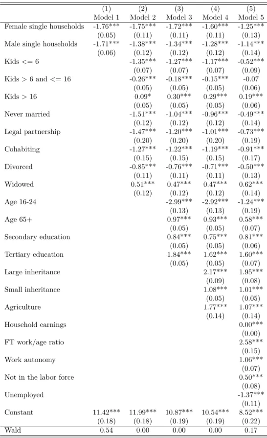
To check the robustness of our OLS analysis in Table 3, we also run a regression on the inverse hyperbolic sine of wealth. The results in Table 4 show that accounting for the non-linearity of the data improves the fit of the model, as expected. The findings of the linear OLS hold qualitatively, and the few unexpected results are reversed. In particular, all unmarried household types have lower wealth compared to married couples, except for widowed reference persons. Young adults have lower net wealth than prime-age reference persons in all models, and households with older reference persons have higher net wealth. Higher education is consistently positively related to effects on net wealth, as is having
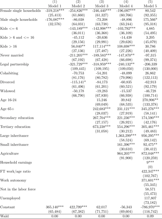
Table 3: OLS Estimates Predicting Household Net Wealth
(1) (2) (3) (4) (5)
Model 1 Model 2 Model 3 Model 4 Model 5 Female single households -319,218*** -254,826*** -246,440*** -196,097*** 80,542
(25,413) (61,660) (61,327) (60,766) (92,355) Male single households -176,087*** -86,038 -73,208 -48,896 175,566* (32,576) (64,031) (63,738) (63,244) (95,318) Kids <= 6 -143,189*** -142,998*** -103,792*** 4,885 (36,011) (36,368) (36,109) (54,495) Kids > 6 and <= 16 -45,112 -20,636 -14,438 3,205 (29,156) (29,991) (29,626) (45,079) Kids > 16 56,040** 117,114*** 108,698*** 30,786 (27,136) (27,487) (27,226) (40,409) Never married -211,205*** -189,583*** -147,870** -97,315 (67,192) (67,428) (66,698) (99,374) Legal partnership -321,729*** -318,959*** -240,132** -206,339 (109,445) (109,195) (109,050) (130,000) Cohabiting -70,753 -54,201 -48,099 26,862 (81,176) (80,782) (79,996) (122,113) Divorced -115,141* -84,173 -60,835 -62,913 (61,496) (61,201) (60,521) (92,179) Widowed -50,178 -19,283 -15,537 -46,728 (66,790) (67,830) (66,938) (100,714) Age 16-24 15,246 39,842 270,906** (69,049) (68,535) (133,378) Age 65+ 242,683*** 231,121*** 345,276*** (28,037) (27,919) (58,141) Secondary education 267,704*** 221,236*** 174,590*** (27,157) (26,921) (42,176) Tertiary education 673,238*** 554,296*** 305,461*** (31,058) (30,212) (49,483) Large inheritance 1,363,299*** 956,295*** (58,524) (69,142) Small inheritance 161,396*** 92,475** (30,610) (38,412) Agriculture 964,205*** 872,048*** (91,900) (120,259) Household earnings 9*** (0) FT work/age ratio 422,347*** (102,767) Work autonomy 371,601*** (55,345)
Not in the labor force 58,571
(55,473) Unemployed 117,807 (73,182) Constant 365,140*** 422,799*** 62,017 -56,343 -786,970*** (65,484) (67,382) (71,751) (69,604) (116,742) Wald 0.00 0.00 0.00 0.00 0.09
received an inheritance. The labor market variables show the expected signs: only having an unemployed reference person is associated with lower net wealth relative to employees. Finally, the IHS results suggest that there is no statistically significant difference between male and female households in our data once all covariates, and in particular labor market effects, are accounted for.
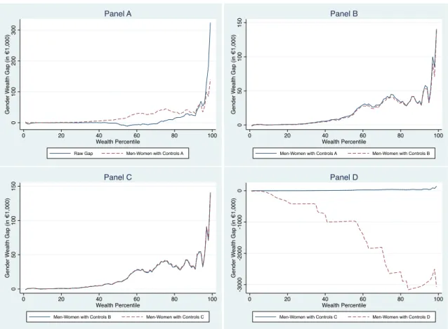
The results of the DFL analysis are presented in Figure 4 on page 20. The solid blue line in the first panel shows the raw wealth gap between male and female households, across the entire wealth distribution. Aside from a small bump into negative territory for the least wealthy households, where male households appear to have more debt than female households, there is hardly any or no gender wealth gap for households in the lower half of the distribution. From about percentiles 50 to 70, female households have a bit more wealth than male households. After that point, male households have increasingly more wealth than female households. The wealthiest male households have more than the wealthiest female households, and this gap grows for each wealth percentile in the distribution. Indeed for the top one or two percent of households, male households have
more thane3m in net wealth more than female households.
The re-weighting applied in the DFL technique makes it possible to ask what the gender wealth gap would be if female households had the same distribution of observable characteristics as male households. These characteristics are introduced in steps, as in the OLS analysis above. In panel A of Figure 4, the weighting is based on household characteristics, namely the probability of having children in the household and of being divorced or widowed. The new distribution is the dotted red line.
Compared to the raw gap, by controlling for these household characteristics the wealth gap for the richest households is reduced somewhat. That is, if female households had the same household characteristics as male households, there would be less of a wealth gap for the richest households. However, along the distribution around the percentiles 30 to 90 (most of the population), a larger wealth gap emerges, wherein male households have more wealth than female households. Thus even if female households had the same rates of parenthood, divorce, widowhood, etc. as men, they would be less wealthy. This finding may be surprising, since women were expected to be less wealthy in part because of their expenses of having children in the household. A potential explanation is that a very large share (almost 75%) of female households have a widowed reference person, and they may have received their partner’s wealth upon their death. Thus if these women had the same (lower) rate of widowhood as men, they would have less wealth.
Panel B shows the distribution of wealth female households would have if they had the same household characteristics, age, and education as male households, compared to the case that they had just the characteristics in control set 1. Here the gender wealth gap declines a bit across the distribution - these characteristics are positively correlated with wealth for male households. In panel C, controls for inheritances are added. Again the gender wealth gap is reduced compared to the case of using control sets 1 and 2, but even adding inheritances cannot explain the gender wealth gap. Indeed controlling for
Table 4: OLS Estimates Predicting IHS Transformation of Household Net Wealth
(1) (2) (3) (4) (5)
Model 1 Model 2 Model 3 Model 4 Model 5 Female single households -1.76*** -1.75*** -1.72*** -1.60*** -1.25*** (0.05) (0.11) (0.11) (0.11) (0.13) Male single households -1.71*** -1.38*** -1.34*** -1.28*** -1.14***
(0.06) (0.12) (0.12) (0.12) (0.14) Kids <= 6 -1.35*** -1.27*** -1.17*** -0.52*** (0.07) (0.07) (0.07) (0.09) Kids > 6 and <= 16 -0.26*** -0.18*** -0.15*** -0.07 (0.05) (0.05) (0.05) (0.06) Kids > 16 0.09* 0.30*** 0.29*** 0.19*** (0.05) (0.05) (0.05) (0.06) Never married -1.51*** -1.04*** -0.96*** -0.49*** (0.12) (0.12) (0.12) (0.14) Legal partnership -1.47*** -1.20*** -1.01*** -0.73*** (0.20) (0.20) (0.20) (0.19) Cohabiting -1.27*** -1.22*** -1.19*** -0.91*** (0.15) (0.15) (0.15) (0.17) Divorced -0.85*** -0.76*** -0.71*** -0.50*** (0.11) (0.11) (0.11) (0.13) Widowed 0.51*** 0.47*** 0.47*** 0.62*** (0.12) (0.12) (0.12) (0.14) Age 16-24 -2.99*** -2.92*** -1.24*** (0.13) (0.13) (0.19) Age 65+ 0.97*** 0.93*** 0.58*** (0.05) (0.05) (0.07) Secondary education 0.84*** 0.75*** 0.81*** (0.05) (0.05) (0.06) Tertiary education 1.84*** 1.62*** 1.60*** (0.05) (0.05) (0.07) Large inheritance 2.17*** 1.95*** (0.09) (0.08) Small inheritance 1.08*** 1.01*** (0.05) (0.05) Agriculture 1.77*** 1.07*** (0.14) (0.14) Household earnings 0.00*** (0.00) FT work/age ratio 2.58*** (0.15) Work autonomy 1.06*** (0.07)
Not in the labor force 0.50***
(0.08) Unemployed -1.37*** (0.11) Constant 11.42*** 11.99*** 10.87*** 10.54*** 8.52*** (0.18) (0.18) (0.19) (0.19) (0.22) Wald 0.54 0.00 0.00 0.00 0.17
inheritances does not change much, suggesting that inheritances do not differ very much by gender (especially once controlling for age).
Finally, panel D adds controls for labor market characteristics, and thus shows the counterfactual wealth distribution of female households if they also had the same
distri-bution of all observable characteristics in the study.5 The results clearly suggest that
differences in the labor market drive much of the gender wealth gap. Along much of the distribution, women would have a very large wealth premium if they had the same char-acteristics as men. These findings are consistent with the literature on the wealth gap (Sierminska et al., 2010), in particular with regard to the large explanatory effect of labor market characteristics.
Figure 4: Wealth in female households, if they had the same distribution of characteristics (sets 2-5) as male households
0 100 200 300 G e n d e r W e a lt h G a p (i n € 1,000) 0 20 40 60 80 100 Wealth Percentile
Raw Gap Men-Women with Controls A Panel A 0 50 100 150 G e n d e r W e a lt h G a p (i n € 1,000) 0 20 40 60 80 100 Wealth Percentile
Men-Women with Controls A Men-Women with Controls B
Panel B 0 50 100 150 G e n d e r W e a lt h G a p (i n € 1,000) 0 20 40 60 80 100 Wealth Percentile
Men-Women with Controls B Men-Women with Controls C
Panel C -3 0 0 0 -2 0 0 0 -1 0 0 0 0 G e n d e r W e a lt h G a p (i n € 1,000) 0 20 40 60 80 100 Wealth Percentile
Men-Women with Controls C Men-Women with Controls D
Panel D
5
Discussion and Conclusions
It is well-documented that wealth is unevenly distributed in society, but there is a large gap in the literature concerning gender differences in wealth. This study used 2010 Household Finance and Consumption Survey data to test for differences in the net wealth
5
The dummy variable for owning an agricultural business had to be excluded from the DFL model, because the final logit regression did not converge with it in. This is likely due to the very small percentage of households, and especially female households, owning an agricultural business.
of households headed by female versus male response persons. We find that overall, male households hold 15% more wealth than female households. Using OLS regressions predict-ing net wealth and the IHS transformation of net wealth, along with a DFL re-weightpredict-ing procedure, we find that the gender wealth gap cannot be explained by differences in house-hold characteristics, the age and education of the respondent, or in inheritances across household types. Instead, it is labor market characteristics which primarily explain the lower levels of wealth found in female households.
This study is the first to test for the presence and extent of a gender wealth gap in Europe. The finding that such a gap exists, but that it would be eliminated if female households had the same characteristics as male households – particularly in labor force participation and in earnings – is striking and important. It may also offer direction for achieving parity in wealth outcomes by gender: if policy can promote labor market equality for men and women, we can take large steps towards reducing gender-based disparity in wealth outcomes. In particular, universally accessible high-quality child care for children of all ages could help reduce these gender gaps in the labor market. Offering child care would allow mothers, who are still generally considered the ones responsible for being primary care-takers, to stay active in the labor market. As more mothers stay at work and fathers bear more responsibility for caring for dependants, prejudices and expectations about women’s lower committment to work would disintegrate, lessening discrimination against them and subsequently raising their pay.
However, some important caveats are in order. There were limitations in the con-struction and implementation of this study, and we therefore must be careful in the in-terpretation of our results. To locate a gender wealth gap, we could only compare wealth
in male and female single households, meaning those who have male and female survey
respondents who were living without a partner present. Thus we are missing any infor-mation on a gender gap which may exist within couples and households. There may also be a selection bias in which men and women head these single households. The gender wealth gap we observe may be due to the mechanisms which make these households sin-gle. If wealthy men and poor women face some selection processes into living without a partner, then we are capturing a story of how households are constructed differently by gender, not one of wealth gaps based on gender differences in wealth accumulation as such. However, we think that it is reasonable to see the story the other way around: people randomly choose how to construct their households and with whom they want to live, and then wealth is accumulated dependent on these choices, not the things which went into household formation processes.
The work presented here has answered some important questions about a gender wealth gap in Europe, but opened the door to ask several others, which future research should address. First, how does the gender wealth gap differ across countries, and how might that be related to policy differences internationally? Second, how has the gender wealth gap developed over time? To the extent that it depends on labor market differences for men and women, as this study suggests, the gender wealth gap is probably at its lowest
point ever. Research to observe the gender wealth gap over time would be able to test the robustness of our finding that the labor market drives the gender wealth gap, but the ability to conduct such research depends on the availability of data to analyze these questions. In this sense, we welcome and encourage the production of more and better data on wealth. In particular, we would benefit from knowing wealth on an individual – not just household – level, as in the German Socio-Economic Panel (see e.g. Wagner et al., 2007). Time series data collecting information on wealth for particular households over a period of time would also be tremendously helpful in understanding the wealth accumulation process. Just as studying pay gaps by gender tells us a great deal about the structure of our society and economy, greater understanding of wealth gaps by gender will illuminate the ways that gender influences economic outcomes.
References
Bardasi, Elena and Janet Gornick, “Working for less? Women’s part-time wage
penalties across countries,”Feminist Economics, 2008, 14(1), 37–72.
Blau, Francine D. and Lawrence M. Kahn, “Swimming Upstream: Trends in the
Gender Wage Differential in 1980s,”Journal of Labor Economics, January 1997,15(1),
1–42.
and , “Gender Differences in Pay,” Journal of Economic Perspectives, 2000, 14(4),
75–99.
Blau, Peter Michael and Otis Dudley Duncan, The American Occupational
Struc-ture, New York: Wiley, 1967.
Bover, Olympia, “Wealth Inequality and Household Structure: U.S. vs. Spain,”Review
of Income and Wealth, 2010, 56(2), 261–290.
Bowles, Samuel and Herbert Gintis, “The Inheritance of Inequality,” Journal of
Economic Perspectives, 2002,16(3), 3–30.
Budig, Michelle J. and Paula England, “The wage penalty for motherhood,”
Amer-ican sociological review, 2001, pp. 204–225.
Burbidge, John B., Lonnie Magee, and A. Leslie Robb, “Alternative
Transforma-tions to Handle Extreme Values of the Dependent Variable,” Journal of the American
Statistical Association, 1988, 83(401), 123–127.
Card, David, “The causal effect of education on earnings,” in O. Ashenfelter and D. Card,
eds., Handbook of Labor Economics, Vol. 3 of Handbook of Labor Economics, Elsevier,
1999, chapter 30, pp. 1801–1863.
Chang, Mariko Lin,Shortchanged: Why women have less wealth and what can be done
about it, New York: Oxford University Press, 2010.
Council of the European Union, “The gender pay gap in the Member States of the European Union: quantitative and qualitative indicators. Belgian Presidency report 2010,” (16516/10 ADD 2 SOC 779), Council of the European Union, Brussels November 2010.
Deere, Carmen Diana and Cheryl R. Doss, “The Gender Asset Gap: What do we
know and why does it matter?,”Feminist Economics, 2006, 12(1-2), 1–50.
and , “Gender and the Distribution of Wealth in Developing Countries,” Working
Paper Series RP2006/115, World Institute for Development Economic Research (UNU-WIDER) 2006.
Denton, Margaret and Linda Boos, “The Gender Wealth Gap: Structural and
Ma-terial Constraints and Implications for Later Life,” Journal of Women & Aging, 2007,
19(3-4), 105–120.
ECB - European Central Bank, “The Eurosystem Household Finance and Consump-tion Survey. Methodological Report for the First Wave,” Statistics Paper Series 1, Eu-ropean Central Bank 2013.
Fernández-Kranz, Daniel and Núria Rodríguez-Planas, “The Part-Time Pay Penalty in a Segmented Labor Market,” IZA Discussion Papers 4342, Institute for the Study of Labor (IZA) August 2009.
Fessler, Pirmin and Martin Schürz, “Reich bleiben in Österreich,” Wirtschaft und
Gesellschaft - WuG, 2013, 39(3), 343–360.
, Peter Mooslechner, and Martin Schürz, “Eurosystem Household Finance and
Consumption Survey 2010. First Results for Austria,”Monetary Policy & the Economy,
2012, (3), 23–62.
Fortin, Nicole, Thomas Lemieux, and Sergio Firpo, “Decomposition Methods in Economics,” Working Paper 16045, National Bureau of Economic Research June 2010.
Frick, Joachim R., Markus M. Grabka, and Richard Hauser,Die Verteilung der
Vermögen in Deutschland: empirische Analysen für Personen und Haushalte, Berlin: edition sigma, 2010.
Gale, William G. and John Karl Scholz, “Intergenerational Transfers and the
Accu-mulation of Wealth,” Journal of Economic P, 1994, 8(4), 145–160.
Gangl, Markus and Andrea Ziefle, “Motherhood, labor force behavior, and women’s careers: An empirical assessment of the wage penalty for motherhood in Britain,
Ger-many, and the United States,”Demography, 2009,46 (2), 341–369.
Gelbach, Jonah B., “When do covariates matter? And which ones, and how much?,” Available at SSRN 2009.
Grabka, Markus M., Jan Marcus, and Eva Sierminska, “Wealth distribution within couples and financial decision making,” CEPS/INSTEAD Working Paper No. 2 2013. Grinstein-Weiss, Michal, Yeon Hun Yeo, Min Yhan, and Pajarita Charles,
“Asset holding and net worth among households with children: Differences by household
type,”Children and Youh Services Review, 2008, 30(1), 62–78.
Hertz, Tom, Tamara Jayasundera, Patrizio Piraino, Sibel Selcuk, Nicole Smith, and Alina Verashchagina, “The Inheritance of Educational Inequality: International
Comparisons and Fifty-Year Trends,”The B.E. Journal of Economics Analysis &
Pol-icy, 2007, 7 (2), Article 10.
Jepsen, Maria, Sile Padraigin O’Dorchai, Robert Plasman, and François Rycx,
“The wage penalty induced by part-time work: the case of Belgium,”Brussels Economic
Review, 2005, 48(1-2), 73–94.
Kotlikoff, Laurence J. and Lawrence H. Summers, “The Contribution of Intergen-erational Transfers to Total Wealth: A Reply,” NBER Working Papers 1827, National Bureau of Economic Research, Inc December 1988.
MacKinnon, James G and Lonnie Magee, “Transforming the Dependent Variable in
Regression Models,”International Economic Review, May 1990, 31(2), 315–39.
Mader, Katharina, Alyssa Schneebaum, Katarina Hollan, and Patricia Klopf, “Vermögensunterschiede nach Geschlecht: Erste Ergebnisse für Österreich aus dem HFCS,” Materialien zu Wirtschaft und Gesellschaft 129, Arbeiterkammer Wien June 2014.
and , “The gendered nature of intra-household decision making in and across
Eu-rope,”Vienna University of Business and Economics Department of Economics Working
Paper, 2013, (157).
Manning, Alan and Barbara Petrongolo, “The Part-Time Pay Penalty for Women in Britain,” CEPR Discussion Papers 6058, C.E.P.R. Discussion Papers January 2007. Matteazzi, Eleonora, Ariane Pailhé, and Anne Solaz, “Part-time wage penalties in Europe: A matter of selection or segregation?,” Working Papers 250, ECINEQ, Society for the Study of Economic Inequality March 2012.
Modigliani, Franco, “The life cycle hypothesis of saving, the demand for wealth and
the supply of capital,”Social Research, 1966,33(2), 160–217. Extracted from PCI Full
Text, published by ProQuest Information and Learning Company.
, “The Role of Intergenerational Transfers and Life Cycle Saving in the Accumulation
of Wealth,”Journal of Economic Perspectives, Spring 1988, 2 (2), 15–40.
Neelakantan, Urvi and Yunhee Chang, “Gender Differences in Wealth at
Retire-ment,” The American Economic Review: Papers and Proceedings, 2010, 100 (2), 362–
367.
Nelson, Julie A., “Are Women Really More Risk-Averse than Men?,” GDAE Working Papers 12-05, GDAE, Tufts University 2012.
Oliver, Melvin and Thomas Shapiro,Black Wealth, White Wealth: A New Perspective
on Racial Inequality, Taylor and Francis, 1997.
Pence, Karen M., “The Role of Wealth Transformations: An Application to Estimating
the Effect of Tax Incentives on Saving,” The B.E. Journal of Economic Analysis &
Policy, July 2006, 5 (1), 1–26.
Pestieau, Pierre, “The Role of Gift and Estate Transfers in the United States and in Europe,” CREPP Working Papers 0202, Centre de Recherche en Economie Publique et de la Population (Research Center on Public and Population Economics) HEC-Management School, University of Liège 2002.
Piketty, Thomas,Capital in the Twenty-First Century, Harvard, 2014.
and Gabriel Zucman, “Capital is Back: Wealth-Income Ratios in Rich Countries,
1700-2010,” Quarterly Journal of Economics, 2014, 129(3), 1255–1310.
, Gilles Postel-Vinay, and Jean Laurent Rosenthal, “Inherited vs. Self-Made Wealth: Theory & Evidence from a Rentier Society (Paris 1872-1937),” CEPR Discus-sion Papers 8411, C.E.P.R. DiscusDiscus-sion Papers Jun 2011.
Plantenga, Janneke and Chantal Remery, “The gender pay gap - Origins and policy responses. A comparative review of 30 European countries,” European Commission, Directorate-General for Employment, Social Affairs and Equal Opportunities 2006.
Ruel, Erin and Robert M. Hauser, “Explaining the Gender Wealth Gap,”
Demogra-phy, 2013,50 (4), 1155–1176.
Schmidt, Lucie and Purvi Sevak, “Gender, Marriage, and Asset Accumulation in the
Schneebaum, Alyssa, Bernhard Rumplmaier, and Wilfried Altzinger, “Gender
in Intergenerational Education Persistence Across Europe,” Vienna University of
Eco-nomics and Business Department of EcoEco-nomics Working Papers, May 2014, (172).
Shenk, Mary K., Monique Borgerhoff Mulder, Gregory Clark Jan Beise, William Irons, Donna Leonetti, Bobbi S. Low, Samuel Bowles, Tom Hertz, Adrian Bell, and Patrizio Piraino, “Intergenerational Wealth Transmission among
Agriculturalists: Foundations of Agrarian Inequality,” Current Anthropology, 2010, 51
(1), 65–83.
Sierminska, Eva, “Does Equal Opportunity Bring Men and Women Closer to Wealth
Equality? Review ofShortchanged: Why Women Have Less Wealth and What Can Be
Done About It,” Review of Income and Wealth, 2014.
, Joachim M. Frick, and Markus M. Grabka, “Examining the gender wealth gap,”
Oxford Economic Papers, 2010, 62(4), 669–690.
Strassmann, Diana, ed.,Feminist Economics2006. 12 (1-2).
Wagner, Gert G., Joachim R. Frick, and Jürgen Schupp, “The German
Socio-Economic Panel Study (SOEP) – Scope, Evolution and Enhancements,” Schmollers
Jahrbuch, 2007, 127 (1), 139–169.
Warren, Tracey, “Moving Beyond the Gender Wealth Gap: On Gender, Class, Ethnicity,
and wealth inequalities in the United Kingdom,” Feminist Economics, 2006, 12 (1-2),
195–219.
Weichselbaumer, Doris and Rudolf Winter-Ebmer, “A Meta-Analysis of the
Inter-national Gender Wage Gap,”Journal of Economic Surveys, 2005, 19(3), 479–511.
Wolff, Edward N., “Recent Trends in the Size Distribution of Household Wealth,”
Journal of Economic Perspectives, 1998, 12(3), 131–50.
Yamokoski, Alexis and Lisa Keister, “The Wealth of Single Women: Marital Status and Parenthood in the Asset Accumulation of Young Baby Boomers in the United