Working-life expectancy in Finland: development in 2000–2009 and forecast for 2010–2015: a multistate life table approach

(1)

FINNISH CENTRE FOR PENSIONS, WORKING PAPERS

Working-life Expectancy in Finland:

Development in 2000–2009

and Forecast for 2010–2015

A Multistate Life Table Approach

Markku Nurminen

Finnish Centre for Pensions

(2)

(3)

Eläketurvakeskus

PENSIONSSKYDDSCENTRALEN

FINNISH CENTRE FOR PENSIONS, WORKING PAPERS

Markku Nurminen

Working-life Expectancy in Finland:

Development in 2000–2009

and Forecast for 2010–2015

(4)

Finnish Centre for Pensions

FI-00065 ELÄKETURVAKESKUS, FINLAND Telephone +358 10 7511 E-mail: [email protected] Eläketurvakeskus 00065 ELÄKETURVAKESKUS Puhelin: 010 7511 Sähköposti: [email protected] Pensionsskyddscentralen 00065 PENSIONSSKYDDSCENTRALEN Telefon: 010 7511 E-post: fö[email protected] Edita Prima Oy Helsinki 2011 ISSN-L 1795-3103 ISSN 1795-3103 (printed) ISSN 1797-3635 (online)

(5)

During the past few years, policy makers have been preoccupied with increasing longevity. Life expectancy has risen rapidly and this development has also affected the views on future population development. The aging of society will have many consequences, but for pension policies it raises the question about the division of time spent in work and in retirement.

Postponing retirement and extending time spent in working-life has become a top priority in most industrialized countries. In Finland, the target is to raise the effective retirement age by three years by year 2025. This target should be seen in the light of a more general employment objective.

The Finnish Centre for Pensions is devoting more research energy to measuring how working careers develop. This Working Paper is part of an on-going partnership project between the Research Department of the Finnish Centre for Pensions and Markstat Consultancy. The research objective is to measure the length of and evaluate the development in working careers – and later and even more ambitiously – to assess the role of pension policy and other contributing factors in the process. This first working paper that springs from the project is devoted to measurement issues and has been written by adjunct professor Markku Nurminen, PhD (Stat.), DrPh (Epid.).

Mikko Kautto

Head of Research Department Finnish Centre for Pensions

(6)

ABSTRACT

Working-life expectancy is the estimated future time that a person will spend in employment. This paper is concerned with its estimation jointly with the time spent in the opposite state of unemployment, and their sum, the expected duration of active working-life, that is, the length of a person’s working career.

This paper employs a multistate method, which has previously been applied to Finnish data from 1980 to 2001. The multistate life table approach first estimates year- and age-dependent probabilities of being in the working-life states by stochastic regression modeling. Updated estimates of probabilities, and subsequently of expectancies, are given for the data of Finnish men and women aged 15–64 years in the period 2000–2009. Further, model-based extrapolations are calculated for the years 2010–2015.

According to results, a general development of longer working careers is evident. During the past decade, the future employment time increased in all age groups and for both genders. For a 15-year-old male in 2009 the fitted estimate of the length of working career is 34.2 years, while for females, it tails at 33.8 years. During the ten-year period 2000–2009, there was an increase of 10 percentage points or more in the expectancies of future working life spent in the employed state for females starting from age 40 and for males from age 50 on.

The respective predicted working-career lengths for 2015 are longer: 36.0 years for males and 35.5 years for females. The female expectancy for ages 40 years and above is forecast to overtake the respective male figure by year 2010 and to continue to do so up to 2015.

Keywords:

• Working-life expectancy • Stochastic inference • Statistics in society

(7)

Työajanodote on luku, joka ilmaisee tietyn ikäisen henkilön jäljellä olevan ajan työelämässä. Tämä tutkimus käsittelee työllisen ajan odotteen, työttömänä oloajan odotteen, sekä niiden yhteenlasketun työvoimaan kuulumisajan odotteen estimointia eli henkilön koko tulevan työuranpituuden mittaamista. Tutkimusmenetelmänä käytettiin tilastotieteellistä monitila-mallia, jota on aiemmin sovellettu Työterveyslaitoksessa käyttäen hyväksi Tilastokeskuksen työvoimatutkimuksen otannan tietoja henkilöiden lukumääristä työmarkkina-aseman mu-kaan ja kuolleisuudesta Suomessa vuosina 1980–2001.

Eläketurvakeskuksen päivitetyssä arvioinnissa laskettiin ensin aineistoon sovitetun sto-kastisen estimointimallin avulla ikä- ja kalenterivuosittaiset todennäköisyydet olla ansio-työssä, työttömänä tai työvoiman ulkopuolella. Todennäköisyyksistä johdettiin integroimal-la odotteet 15–64-vuotialle suomaintegroimal-laisille miehille ja naisille vuosina 2000–2009. Odotteiden ennustemalliin perustuvat eskstrapolaatiot projisoitiin vuosille 2010–2015.

Tulosten mukaan yleinen positiivinen kehitys kohti pidempiä työuria on ilmeistä. Viime vuosikymmenen kuluessa jäljellä oleva työssäoloaika kasvoi molemmilla sukupuolilla kai-kissa ikäryhmissä. 15-vuotiaiden miesten työajanodote oli lamavuonna 2009 mallin antaman arvion mukaan 34,2 vuotta, naisten odote oli hieman lyhyempi eli 33,8 vuotta. 10-vuoden ajanjaksolla 2000–2009 työajanodotteen kasvu oli naisilla 10 %-pistettä tai enemmän alka-en ikävuodesta 40, miehillä ikävuodesta 50 lähtialka-en. Yli 40-vuotiaittalka-en naistalka-en odottealka-en alka- en-nustettiin ylittävän miesten vastaavan odotteen vuoteen 2010 mennessä. Ennusteet 15-vuoti-aiden henkilöiden työurien kestoille vuonna 2015 ovat entistä pidempiä (olettaen kehityksen jatkuvan samansuuntaisena): miehillä 36,0 vuotta, naisilla lähes yhtä pitkä eli 35,8 vuotta. Avainsanat:

• Työajanodote • Stokastinen päätäntä • Tilastotiede yhteiskunnassa

(8)

ACKNOWLEDGMENTS

Dr. Brett A. Davis, Australian Government Department of Employment and Workplace Relations, Canberra, ACT, gave invaluable expert advice in the application of stochastic processes to life sciences.

Dr. Martin Tondel, Section of Occupational and Environmental Medicine, Department of Public Health and Community Medicine, Institute of Medicine, University of Gothenburg, Gothenburg, Sweden, contributed useful methodological points on the validity of the official data used for predicting the working-life expectancies.

Suvi Pohjoisaho, Publications Assistant at the Finnish Centre for Pensions, has taken care of transforming the manuscript into a publication.

Statistics Finland provided the population employment data on labor force and mortality rates.

(9)

1 Introduction...9

2 Official Data...13

3 Outline of the Method...16

4 Estimates of Model Parameters...18

5 Estimates of State Probabilities...21

6 Estimates of Working-life Expectancies...24

7 Forecasts of Working-life Expectancies...32

8 Discussion...36 8.1.Longer.Working.Lives.Tackle.Aging.Societies...36 8.2.Prevalence.versus.Multistate.Life.Table.Analysis...37 9 Methodological Recommendations...40 Appendices...41 Appendix.A:.Details.of.Modeling.and.Estimation.Methods...41 Appendix.B:.Forecasting.from.the.Regression.Model...44 Appendix.C:.Approaches.to.Setting.Prediction.Intervals...45 References...47

(10)

(11)

1 Introduction

Extending working-life has become a strategic objective in many industrialized countries facing budgetary concerns in the foresight of the demographic aging. Population aging is likely to lead to lower productivity both because the workforce grows older and because a lower proportion of the population is working. Shorter working lives, coupled with increased life expectancy, low fertility and the retirement of the large post-war generation, have an ageing and shrinking effect on the economically active share of the population. This will have major implications for work productivity and overall economic growth (Skirbekk, 2005).

The increase in life expectancy in Finland has been more rapid than projected, resulting in a situation where pension expenditure will be higher than was predicted at the time of planning the 2005 pension reform, unless working careers grow longer accordingly. Measures aimed at lengthening working careers can be divided into two groups: measures related to developing working life and measures aimed at developing pension systems (Prime Minister’s Office, 2010).

The Finnish Government and the labor market organizations have agreed that the expectancy for the effective retirement age for 25-year-olds should be raised from 59.4 (in 2008) by at least 3 years by year 2025.

The question of postponing retirement should be seen in the context of the entire working career. The working group considering working careers from the perspective of the earnings-related pension scheme held it essential that the length of the working career should not be measured singularly based on the expected exit age to retirement. This measure should be complemented with the expectation of active working life and employment rate (Prime Minister’s Office, 2011.)

At present in Finland there are different statistical indicators in use that measure the duration of various phases in life from the separate perspectives of the pension system and the labor market (for a review, in Finnish, see Hytti, 2009). The Finnish Centre for Pensions (Eläketurvakeskus, ETK) has computed the expected effective retirement age indicator (Kannisto, 2006), and later complemented it by publishing the expected duration of employment (or active working-life) indicator developed by Helka Hytti and Ilkka Nio (2004). The former indicator is based on data on insured persons moving into earnings-related pension, and it is computed from age-specific transition frequencies into retirement and from mortality statistics.

The latter indicator is suitable in planning labor force policies and in assessing the efficiency of employment programs. However, this working-life expectancy is preferably estimated from the total population probabilities of being in the three mutually exclusive states of employed, unemployed, and outside the labor force (e.g. on disability pension), rather than just in the two classes of active and inactive, as has been previously customary.

Recently, the EU Commission’s study has recommended using the duration of working-life expectancy, which partitions the working-life expectancy into separate working-life stages, as a core labor market indicator at European and Member State level (Vogler-Ludwig and Düll, 2008). The expert consultants’ report suggests that the application of the expectancy would appear to be

(12)

10 FINNISH CENTRE FOR PENSIONS, WORKING PAPERS

useful for the description and analysis of long-term behavioral and institutional conditions in national employment systems rather than for the monitoring of short-term changes.

For a worker of a given initial age, working-life expectancy (WLE) is the expected future time a person spends in gainful employment earning wages and benefits (or looking for work) assuming that the prevailing patterns of mortality, morbidity and disability remain unchanged (Nurminen, 2008). It is a period or cohort measure, depending on whether cross-sectional or longitudinal data are available. Life expectancy at birth is naturally somewhat different to that calculated for an actual cohort at the start of follow-up (Myrskylä, 2010).

Usually, in the case of WLE studies, only cross-sectional data from official statistics can be readily obtained (cf. Nurminen et al., 2004a). This situation is similar to the usual circumstances in which life expectancy is calculated. Our interest in this Working Paper is in WLE and similar expectations of times spent in states other than employment, such as unemployment, or being temporally or permanently outside the labor force (e.g. in rehabilitation or on disability pension). The estimation of expectations is conditional on having reached a given age. For persons of working age these expectations are termed

partial life expectancies.

In our previous cohort follow-up study (Nurminen et al., 2004) of initially active Finnish municipal workers, aged 45 to 58 years in 1981, we assumed that the earliest commencing date in employment is in the middle of the initial age interval (45–46), and that the retirement date is no later than the 63rd birthday. Thus the maximum duration of work for the cohort members was 17.5 years. The effective expected retirement age was 59.8 or approximately 60 years in Finland in 2009 (Finnish Centre for Pensions, 2011). We found that men permanently leave the work force due to disability or death earlier than women in all age groups, regardless of whether they commenced in better or worse work ability (Nurminen et al., 2004b). Women tended to retire on old-age or similar pension before men, especially those women with an initially fair or poor capacity for work. The cross-sectional survey data suggested that the work ability of Finnish aging workers appears to deteriorate prematurely and that individuals leave too frequently employment before the statutory retirement age. Rather remarkably, the work-physiological effect of transition at the age of 45 years from the initial state of ’poor’ to ’good or excellent’ work ability was estimated to be, on average, four years of gained active work life for both genders. Such an achieved improvement would mean that an advancement of the expectancy for the effective

retirement age can conceivably reach a higher target than that set for the year 2025, viz. 62.4 years, because 60 + 4 = 64; hence it could also exceed the current lower limit of the

(13)

Figure 1.

WLE of male municipal workers by their work ability and age.

45 46 47 48 49 50 51 52 53 54 55 56 57 58 59 60 61 62 Age, years 0 2 4 6 8 10 Ex pectancy , y ears

Working Life Expectancy by Work Ability Status

Good work ability Fair work ability Poor work ability

In Figure 1, the WLEs are plotted along the age axis with the subsequent values for fair work ability and good work ability ’stacked’ on top of the previous ones. E.g., at 45 years, an ’average’ male worker is expected to be employed 5.5 (= 11.5 – 6.0) years with ’good or excellent’, 4.5 (= 6.0 – 1.5) years with ’fair’, and 1.5 years with ’poor’ work ability. The

WLEs add up to 5.5 + 4.5 + 1.5 = 11.5 years. Six years is spent outside work life before the retirement at age of 62.5 (= 45 + 11.5 + 6.0) years. Note that the expectations add up to the duration of maximum remaining work life at age 45, taken as 17.5 (= 63 – 45 – ½) years; ½ is subtracted since persons enter work on average in the middle of the age interval (45, 46).

The additive partition of the WLEs in relation to the specified levels of work ability is an appealing methodological property of the WLE measure. The decomposition is helpful in understanding at what stages changes in people’s health are occurring and in quantifying the magnitude of those transitions conditionally on the initial work ability.

The present paper is concerned with the joint estimation by year and age of the probabilities and expectancies of working-life states. We applied a modern regression model to cross-sectional life table data from Finland for each of the years 2000 to 2009 with projections to 2010–2015. Our estimates are for ages 15 to 64 inclusive, conditional only on a person being alive at age 15. We used the multistate life table modeling approach (Davis

et al., 2001) to overcome certain limitations of the traditional prevalence life table technique (Hytti and Nio, 2004). The stochastic modeling approach yields a wealth of information about working-life behavior when applied to intrinsically dynamic life processes with multiple decrements, like the labor force process. Thus, for instance, it is possible to test statistically the effect (trend change) of the pension reform that was enforced in 2005 on the

WLEs.

Working-life and related expectancies are conceptually analogous to health expectancies, both representing expected occupation times; the difference is that the former arise in the context of labor force activity rather than health status. Consequently, given a suitable

(14)

formulation of the problem, similar methods of analysis can be used, and we employ the large-sample, weighted least squares version of logistic regression modeling originally developed for the Australian health surveys by Davis et al. (2001, 2002b). This statistical framework is different to the frequency-based methods previously applied to health expectancies (Sullivan, 1971). A bibliography can be found in the handbook of Réseau sur l’Espérance de Vie en Santé, REVES (2002).

Given discrete-time data from multiple cross-sectional population surveys, a multistate regression model can be used to estimate consistently marginal probabilities that a person is in a given work-health state or transition probabilities between the states, and, thereby, working-life expectancies (Nurminen and Nurminen, 2005). Expectancies conditional on an initial state and based on transition probabilities can be estimated under the Markov assumption from aggregate data that are produced by official statistical agencies’ longitudinal time series and were presented and applied in Davis et al. (2002a, 2000b, and 2007).

This paper is organized as follows: Section 1 briefly reviews the background to the topic and introduced the working-life expectancy for measuring the future career length. The official data used in the study are described in Section 2. Section 3 presents an outline of the statistical methodology. Estimates of the model parameters are given in Section 4, those of the state probabilities in Section 5, while Section 6 presents current estimates of

WLEs, followed by forecasts of the WLEs in Section 7. Finally, Section 8 discusses the results obtained using modern regression and compares them to those obtained by actuarial techniques. Section 9 proposes recommendations on the applicable methodology. Statistical modeling, estimation, and prediction issues are detailed in the Appendices.

(15)

2 Official Data

Estimates of the sizes of the Finnish populations for the years 2000–2009, by labor force status, sex and single-year working-age groups, taken from 15 to 64, were provided by the Information Services of Statistics Finland (SF, 2010) based on the Labour Force Survey (LFS) data. In all, the data set consisted of a four-dimensional array of 4,000 frequencies indexed by sex, age (15–64 years), calendar year (2000–2009), and labor force status. Annual Gross Domestic Product (GDP) (as of July 1, 2011) was included as an explanatory variate in the regression model.

The Finnish LFS collects statistical data on the participation in work, employment, unemployment and activity of persons outside the labor force, among the population aged between 15 and 74. The LFS data acquisition is based on a random sample drawn twice a year from the population database. The monthly sample consists of some 12,000 persons and the data are obtained by means of computer-assisted telephone interviews. The information given by the respondents is used to produce a representative picture of the activities of the entire working-age population.

The concepts and definitions used in the Survey comply with the recommendations of ILO, the International Labour Organisation of the UN, and the regulations of the European Union on official statistics. The quality of the LFS is described in detail by SF (2011).1

The numbers of annual deaths in the study years were extracted from the files kept by Statistics Finland. The statistics on deaths cover persons permanently domiciled in Finland. Data on the population and age and gender distribution of deaths are used to calculate annual figures on life expectancy.

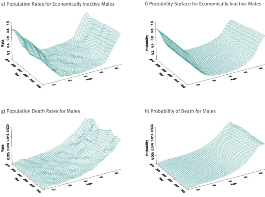
Figure 2 shows the actual observations which we used to estimate probabilities and expectancies. The fitted values were smoothed by Friedman’s local regression spline function. Our interest focused on the three mutually exclusive states: ’employed’, ’unemployed’, and ’economically inactive’. This complementary ’inactive’ or ’other alive’ group represents a mixed population and includes persons who are outside the labor force; that is, those individuals who are not employed or unemployed during the survey week, on pensions due to various causes of disability, as well as students, conscripts and civil servants. ’Deceased’ was taken as a reference state.

1 The Ministry of Employment and the Economy also publishes data on unemployed job seekers. The Ministry’s data derive from register-based Employment Service Statistics, which describe the last working day of the month. The definition of unemployed applied in the Employment Service Statistics is based on legislation and administrative orders which make the statistical data internationally incomparable. In the Employment Service Statistics an unemployed person is not expected to seek work as actively as in the Labour Force Survey. There are also differences in the acceptance of students as unemployed.

(16)

Figure 2.

Population rates (per 1,000 people) and probability surfaces fitted by a Friedman’s smoothing spline function for (1) males and (2) females:

(a) observed, employed (b) fitted, employed (c) observed, unemployed (d) fitted, unemployed (e) observed, inactive (f) fitted, inactive (g) observed, deceased (h) fitted, deceased Figure 2.1

Males

c) Population Unemployment Rates for Males d) Probability Surface of Unemployment for Males a) Population Employment Rates for Males b) Probability Surface of Employment for Males

e) Population Rates for Economically Inactive Males f) Probability Surface for Economically Inactive Males

(17)

Figure 2.2 Females

a) Population Employment Rates for Females b) Probability Surface of Employment for Females

e) Population Rates for Economically Inactive Females f) Probability Surface for Economically Inactive Females

g) Population Death Rates for Females h) Probability of Death for Females

(18)

3 Outline of the Method

It is convenient to describe the method used in terms of a population cohort of n lives initially aged 15 years. Of particular importance are the probabilities that an individual is in state j

at a subsequent age x, written p_j(x). In the present application, j = 0 denotes ’alive’ and j = 1,2,3,4 indexes the exhaustive (non-overlapping) states (1) ’employed’, (2) ’unemployed’, (3) ’economically inactive’, and (4) ’dead’. Here our interest is on estimating the marginal probabilities and working-life expectancies that are not conditional on the initial state, but only on the initial age. Aggregate data were available at ages x = 15, ..., 64.

Estimation of the unconditional probabilities p_j(x) is done by a large-sample version of logistic regression. We shall call p₁(x) the working life survival curve. Advantage is taken of the fact that official statistics are almost always given in terms of large numbers, which in the present case translates as large n, the number of individuals in the cohort. The theoretical premises of the method are given in Davis et al. (2001, 2002b), and in some detail in Appendix A.

With state 4 (dead) as the reference, we formed the log ratios

      

3 Outline of the Method

It is convenient to describe the method used in terms of a population cohort of n lives initially aged 15 years. Of particular importance are the probabilities that an individual is in state j at a subsequent age

x, written pj(x). In the present application, j = 0 denotes 'alive' and j = 1,2,3,4 indexes the exhaustive (non-overlapping) states (1) 'employed', (2) 'unemployed', (3) 'economically inactive', and (4) 'dead'. Here our interest is on estimating the marginal probabilities and working-life expectancies that are not conditional on the initial state, but only on the initial age. Aggregate data were available at ages x = 15, ..., 64.

Estimation of the unconditional probabilities pj(x) is done by a large-sample version of logistic regression. We shall call p1(x) the working life survival curve. Advantage is taken of the fact that official statistics are almost always given in terms of large numbers, which in the present case translates as large n, the number of individuals in the cohort. The theoretical results of the method are given in Davis et al. (2001, 2002b), and in some detail in Appendix A.



= log{pj(x)/p4(x)}, j = 1,2,3. (Eq 1)

Exploratory analysis can be used to suggest a parametric form for the partial log ratios, _ξ(x) ≡_ξ(x;

β), and the estimation of β is done by weighted least squares. With the resulting estimate of β we have the derived parameter estimates

 (x) =

_

(x;_), j pˆ (x) =

ˆp

4(x) exp[xˆj(x)], j = 1,2,3, (Eq 2) 4

ˆp

(x) = {1 +∑ exp  [(x)]}-1 .

Thence the estimated working life and related expectancies of interest (for a given age z) are defined as a definite integral function

j eˆ (z) =

∫

64

)

(

ˆ

z j

x

dx

p

. (Eq 3)

The expectation of main interest, e1, yields the working life expectancy (WLE). These quantities are conditional only on the fact that an individual is alive at age 15, and they should be distinguished

(Eq 1) Exploratory analysis can be used to suggest a parametric form for the partial log ratios,

(x) ≡ (x; β), and the estimation of β is done by weighted least squares. With the resulting estimate of β we have the derived parameter estimates

(Eq 2)                   

 (x) =

_

(x;_), j pˆ (x) =

ˆp

₄(x) exp[xˆ_j(x)], j = 1,2,3, (Eq 2)       

3 Outline of the Method



= log{pj(x)/p4(x)}, j = 1,2,3. (Eq 1)

Exploratory analysis can be used to suggest a parametric form for the partial log ratios, _ξ(x) ≡_ξ(x;

β), and the estimation of β is done by weighted least squares. With the resulting estimate of β we have the derived parameter estimates

 (x) =



(x;_), j pˆ (x) =

ˆp

4(x) exp[xˆj(x)], j = 1,2,3, (Eq 2) 4

ˆp

(x) = {1 +∑ exp  [(x)]}-1 .

j eˆ (z) =

∫

64

)

(

ˆ

z j

x

dx

p

. (Eq 3)

Thence the estimated working life and related expectancies of interest (for a given age z) are defined as a definite integral function

      

3 Outline of the Method



= log{pj(x)/p4(x)}, j = 1,2,3. (Eq 1)

Exploratory analysis can be used to suggest a parametric form for the partial log ratios, _ξ(x) ≡_ξ(x; β), and the estimation of β is done by weighted least squares. With the resulting estimate of β we have the derived parameter estimates

 (x) =



(x;_), j pˆ (x) =

ˆp

₄(x) exp[xˆ_j(x)], j = 1,2,3, (Eq 2) 4

ˆp

(x) = {1 +∑ exp  [(x)]}-1 .

j eˆ (z) =

∫

64

)

(

ˆ

z j

x

dx

p

. (Eq 3)

(Eq 3)

The expectation of main interest, e₁, yields the working life expectancy (WLE). These quantities are conditional only on the fact that an individual is alive at age 15, and they should be distinguished from working life expectancies conditional on knowledge of the initial work-life or health state. Observe that the expectation e₀ = Σ3

j=1ej is the partial life

expectancy to age 65 for an individual known to have been alive at 15, and that Σ4

j=1ej = 50.

The large-sample arguments apply to estimating current survival curves and expectancies as functions of age for a given year. However, we had data available for the decade 2000 to 2009 and clearly variation with year is also of interest. It is therefore natural to model the

(19)

vector of log ratios as a function of both year t and age x, (t,x), bearing in mind that only cross-sectional data are available.

We also used the S-PLUS program function predict on a generalized linear model object to compute preliminary predicted values for working-life expectancies in a new data frame containing the values at future time points as well as their associated prediction intervals (see Appendix C).

(20)

4 Estimates of Model Parameters

A variety of plausible models can be used to describe the same data. Our selection of a multistate model for the four states required the estimation of 33 separate sets of parameters for both genders. The choice of the model covariates was based on significance testing using the original standard errors (uncorrected for population heterogeneity). To motivate the argument, the observed rates for 2009 plotted in Figure 2 were considered. Upon examination of the contours of the surfaces, a cubic function at age x for the log ratios was estimated from the numbers. Similar results were obtained for other years.

Recession effects, episodes of unemployment, effects of the Finnish new pension law (which was put in force in 2005) and interaction effects enter into the formulation of models incorporating change both with year as well as age. The left hand columns of Figures 2.1 and 2.2 give the observed frequency rates. Some experimentation led to the fitted model parameters listed in Tables 1 and 2 (9 + 12 + 12 = 33 parameters for the male odds ratios and 10 + 11 + 12 = 33 for the female log ratios) together with their standard errors. Specifically,

to describe the particular behavior of the estimates at the youngest and oldest ages, we included indicators for the age groups 15–17 and 60+. Also an indicator was entered in the model for the years following 2005, when the new pension law was enacted in Finland. For men, the effect was significant for the states of ’unemployed’ and economically ’inactive’ (Table 1) and for women for the state of ’inactive’ (Table 2). The final model form is specified in Appendix A.

Substitution in Equation 1 gives the fitted probability surfaces (interpolating through data points by means of a cubic spline) shown in the right hand column of Figures 2.1 and 2.2. Numerical values of the estimated model parameters with their standard errors are given in Table 1 for males and in Table 2 for females.

(21)

Table 1.

Regression model parameter estimates and standard errors of the three working-life states for males.

Regression term

Results for state employed Results for state unemployed Results for state inactive Parameter Estimate Standard _error Parameter Estimate Standard _error Parameter Estimate Standard _error Intercept (mean) β1 6.06e+0 1.86e-1 β10 3.27e+0 1.96e-1 β22 3.32e+0 1.91e-1

Age (centered at

39.5 years), x β2 -7.35e-2§ 2.00e-2 β11 -6.95e-2 2.05e-2 β23 -4.68e-2 2.01e-2

Squared term, x2 _β

3 -2.67e-3 8.13e-4 β12 8.13e-5 8.32e-4 β24 4.01e-3 8.18e-4

Cubic term, x3 _β

4 4.41e-5 5.99e-5 β13 -3.50e-5 6.17e-4 β25 5.55e-5 6.01e-5

Teen age indicator,

I(15 ≤ x ≤ 17) * β14 -1.68e-1 1.48e-1 β26 2.18e-1 9.61e-2

Senior age

indicator, I(x ≥ 60) β5 -3.38e-1 3.92e-1 β15 -9.30e-1 4.32e-1 β27 1.85e-1 3.94e-1

Calendar year

(ordinally scaled), t β6 1.86e-2 6.04e-2 β16 -2.86e-2 6.56e-2 β28 2.13e-2 6.38e-2

Interaction effect

product term, tx β7 9.64e-4 2.61e-3 β17 -1.66e-3 6.18e-3 β29 -7.75e-4 6.07e-3

Squared term, tx2 _β

8 1.84e-5 1.60e-4 β18 8.12e-5 2.65e-4 β30 -4.27e-5 2.61e-4

Cubic term, tx3 _β

9 4.41e-6 7.14e-5 β19 4.67e-6 1.64e-5 β31 8.39e-8 1.60e-5

Pension year indicator

I(2005 ≤ t ≤ 2010) *

β20 -8.77e-2 9.71e-2 β32 -5.22e-2 6.58e-2

Gross domestic

product, GDP * β21 -2.60e-2 7.69e-3 β33 4.57e-3 5.11e-3

§_{Exponential notation, e.g., −7.35e − 2 = −7.35 x 10–2 = −0.0735}

(22)

Table 2.

Regression model parameter estimates and standard errors of the three working-life states for females.

Regression term

Results for state employed Results for state unemployed Results for state inactive Parameter Estimate Standard _error Parameter Estimate Standard _error Parameter Estimate Standard _error Intercept (mean) β1 6.81e+0 3.09e-1 β11 4.09e+0 3.12e-1 β22 4.82e+0 3.12e-1

Age (centered at

39.5 years), x β2 -6.39e-2§ 3.26e-2 β12 -8.07e-2 3.29e-2 β23 -1.10e-1 3.27e-2

Squared term, x2 _β

3 -1.88e-3 1.54e-3 β13 5.97e-5 1.55e-3 β24 2.38e-3 1.54e-3

Cubic term, x3 _β

4 -1.27e-5 1.05e-4 β14 -2.96e-5 1.06e-4 β25 8.84e-5 1.05e-4

Teen age indicator,

I(15 ≤ x ≤ 17) β5 -8.84e-1 2.06e-0 β15 -5.15e-1 2.06e-0 β26 5.27e-1 2.06e-0

Senior age

indicator, I(x ≥ 60) β6 -3.99e-1 5.96e-1 β16 -1.04e+0 6.26e-1 β27 1.89e-1 5.97e-1

Calendar year

(ordinally scaled), t β7 3.04e-2 9.95e-2 β17 -2.24e-2 1.00e-1 β28 3.33e-2 1.00e-1

Interaction effect

product term, tx β8 -3.37e-3 9.66e-3 β18 -2.49e-3 9.75e-3 β29 -3.06e-3 9.68e-3

Squared term, tx2 _β

9 1.31e-5 4.17e-4 β19 1.59e-5 4.20e-4 β30 -1.05e-4 4.17e-4

Cubic term, tx3 _β

10 1.13e-5 2.49e-5 β20 7.73e-6 2.52e-5 β31 6.39e-6 2.49e-5

Pension year indicator

I(2005 ≤ t ≤ 2010) * *

β32 -5.10e-2 6.02e-2

Gross domestic

product, GDP * β21 -6.05e-3 7.45e-3 β33 9.91e-4 4.76e-3

§_{Exponential notation, e.g., −6.39e − 2 = −6.39 x 10 – 2 = −0.0639}

(23)

The Working-life Expectancy in Finland 2000–2015 21

5 Estimates of State Probabilities

Numerical values for the estimated probabilities of the four occupancy states are given in Table 3 separately for (a) males and (b) females.

After the economic downturn in 2001–2003, the estimated probabilities of being employed increased rather consistently between the years 2000–2008 in all age groups and for both genders, whereas the probabilities of unemployment diminished.

The severe economic recession that started in the late 2008 led to an exceptionally sharp drop in GDP (-8 %), followed by a fairly rapid rebound in the probability of employment in around 2009. Conversely, the probabilities of unemployment were markedly greater than the estimates for the years neighboring 2009. The recession effect was more significant for men than for women. This effect bears some consequences to 2010 and to the following years.

In Table 3a and Table 3b the one-year-ahead forecasts of the work life state probabilities for the year 2010 were determined by estimating parameters from all the data in the interval from 2000 up to 2009. The entries for the estimated probabilities in the columns for 2010 were obtained by first extrapolating the regression fits to the log ratios within the sample and using these to give projected probabilities and thereby expectancies.

These projections are thus essentially those given by standard regression methods. No attempt was made to forecast by altering regression coefficients to reflect possible future case scenarios. The standard errors for the probabilities in Table 3a and Table 3b are not exhibited to conserve space.

Large-sample significance tests can easily be constructed. To take a particular case, consider the difference between males and females in the probability of employment in the economic recession year 2009. The gender difference for an ”average” (or randomly chosen) 25-year-old male worker was greater than that for women (Table 3a and Table 3b):







5 Estimates of State Probabilities

Numerical values for the estimated probabilities of the 4 occupancy states are given Table 3 separately for (a) males and (b) females.

After the economic downturn in 2001-2003, the estimated probabilities of being employed increased rather consistently between the years 2000-2008 year in all age groups and for both genders, whereas the probabilities of unemployment diminished.

The severe economic recession that started in the late 2008 led to an exceptionally sharp drop (GDP = -8%) and then a fairly rapid rebound in the probability of employment occurred in around 2009. Conversely, the probabilities of unemployment were markedly greater than the estimates for the years neighbouring 2009. The bulge was more significant for men than for women. This effect carries a weakening aftermath to 2010 and to the following years.

In Table 3 a and Table 3 b the one-year-ahead forecasts of the worklife state probabilities for the year 2010 were determined by estimating parameters from all the data in the interval from 2000 up to 2009. The entries for the estimated probabilities in the columns for 2010 were obtained by first extrapolating the regression fits to the log ratios within the sample and using these to give projected probabilities and thereby expectancies.

These projections are thus essentially those given by standard regression methods. No attempt was made to forecast by altering regression coefficients to reflect possible future case scenarios. The standard errors for the probabilities in Table 3 a and Table 3 b are not exhibited to conserve space.

Large-sample significance tests can easily be constructed. To take a particular case, consider the difference between males and females in the probability of employment in the economic recession year 2009. The gender difference for an "average" (or randomly chosen) 25-year old male worker was greater than that for women (Table 3 a and Table 3 b):

̂₁M,2009(25) - _̂₁F,2009(25) = 0.7275 – 0.6466 = 0.0809

The standard error of the difference was estimated by computing the variance-covariance matrix for the fitted probabilities (using the Liang-Zeger delta method modified for the heterogeneous aggregate data):

SE{_̂₁M,2009(25) - _̂₁F,2009(25)} = {SE[_̂₁M,2009(25)]2_{+ SE[}_̂ ,2009 1

F

(25)]2_}½

= (0.010822_{+ 0.01142}2₎½_{= 0.0157}







5 Estimates of State Probabilities

Numerical values for the estimated probabilities of the 4 occupancy states are given Table 3 separately for (a) males and (b) females.

After the economic downturn in 2001-2003, the estimated probabilities of being employed increased rather consistently between the years 2000-2008 year in all age groups and for both genders, whereas the probabilities of unemployment diminished.

The severe economic recession that started in the late 2008 led to an exceptionally sharp drop (GDP = -8%) and then a fairly rapid rebound in the probability of employment occurred in around 2009. Conversely, the probabilities of unemployment were markedly greater than the estimates for the years neighbouring 2009. The bulge was more significant for men than for women. This effect carries a weakening aftermath to 2010 and to the following years.

In Table 3 a and Table 3 b the one-year-ahead forecasts of the worklife state probabilities for the year 2010 were determined by estimating parameters from all the data in the interval from 2000 up to 2009. The entries for the estimated probabilities in the columns for 2010 were obtained by first extrapolating the regression fits to the log ratios within the sample and using these to give projected probabilities and thereby expectancies.

These projections are thus essentially those given by standard regression methods. No attempt was made to forecast by altering regression coefficients to reflect possible future case scenarios. The standard errors for the probabilities in Table 3 a and Table 3 b are not exhibited to conserve space.

Large-sample significance tests can easily be constructed. To take a particular case, consider the difference between males and females in the probability of employment in the economic recession year 2009. The gender difference for an "average" (or randomly chosen) 25-year old male worker was greater than that for women (Table 3 a and Table 3 b):

̂₁M,2009(25) - _̂₁F,2009(25) = 0.7275 – 0.6466 = 0.0809

SE{_̂₁M,2009(25) - _̂₁F,2009(25)} = {SE[_̂₁M,2009(25)]2_{+ SE[}_̂ ,2009 1

F

(25)]2_}½

= (0.010822_{+ 0.01142}2₎½_{= 0.0157}

The difference in the probabilities is multiple times as large as the normal (Gaussian) standard deviation. This test realization corresponds to the two-tailed P-value < 0.001. So the gender gap in employment probabilities was still statistically highly significant, although men typically suffer more from jobs lost in recession. On the other hand, while the estimated probability of employment for 25-year-old men was predicted to rebound from 0.7275 in 2009 to 0.7539 in 2010, no such ascent was foreseen for women (0.6466 in 2009 vs. 0.6480 in 2010).

(24)

Table 3a.

Fitted probabilities for men of the four states 1 = ’employed’, 2 = ’unemployed’, 3 = ’economically inactive’, and 4 = ’dead’, expressed as percentages, with projections for 2010, for selected years and ages. Age x State j Men 2001 2003 2005 2007 2009 2010 15 1 9.35 8.95 9.06 8.79 7.82 8.15 2 6.80 6.61 6.03 5.53 7.01 5.47 3 83.81 84.41 84.88 85.64 85.14 86.35 4 0.03 0.03 0.03 0.03 0.03 0.03 20 1 44.07 43.83 45.33 45.66 42.51 44.91 2 12.61 12.35 11.16 10.31 13.25 10.34 3 43.22 43.72 43.41 43.93 44.15 44.66 4 0.10 0.10 0.10 0.10 0.09 0.09 25 1 72.56 72.84 74.60 75.41 72.75 75.39 2 9.90 9.53 8.31 7.51 9.74 7.36 3 17.42 17.51 16.97 16.97 17.41 17.14 4 0.13 0.12 0.12 0.12 0.11 0.11 30 1 84.12 88.21 85.92 86.65 84.84 86.84 2 7.38 5.84 5.90 5.21 6.72 4.96 3 8.36 5.79 8.05 8.01 8.32 8.09 4 0.14 0.16 0.13 0.13 0.12 0.12 35 1 87.80 88.39 89.42 90.08 88.65 90.30 2 6.29 5.66 4.86 4.22 5.39 3.93 3 5.74 5.72 5.56 5.55 5.81 5.63 4 0.17 0.22 0.16 0.15 0.14 0.14 40 1 87.96 85.95 89.60 90.24 88.90 90.47 2 6.15 6.04 4.67 4.02 5.09 3.69 3 5.66 7.67 5.52 5.52 5.82 5.64 4 0.23 0.33 0.22 0.21 0.20 0.20 45 1 85.48 80.04 87.31 88.02 86.58 88.29 2 6.58 6.59 4.98 4.27 5.38 3.91 3 7.60 12.84 7.38 7.38 7.73 7.50 4 0.34 0.53 0.33 0.32 0.31 0.31 50 1 79.42 80.04 81.77 82.69 81.14 83.16 2 7.13 6.59 5.48 4.74 5.98 4.37 3 12.90 12.84 12.22 12.05 12.39 11.98 4 0.54 0.53 0.53 0.52 0.49 0.50 55 1 67.29 68.48 71.07 72.63 71.43 73.95 2 7.04 6.64 5.67 5.01 6.40 4.75 3 24.79 24.03 22.42 21.54 21.41 20.53 4 0.87 0.85 0.84 0.81 0.76 0.77 60 1 36.41 38.97 43.02 46.06 47.01 49.91 2 2.31 2.34 2.16 2.04 2.75 2.11 3 59.92 57.37 53.48 50.60 49.02 46.74 4 1.35 1.32 1.33 1.31 1.22 1.24

(25)

Table 3b.

Fitted probabilities for women of the four states 1 = ’employed’, 2 = ’unemployed’, 3 = ’economically inactive’, and 4 = ’dead’, expressed as percentages, with projections for 2010, for

selected years and ages. Age x State j Women 2001 2003 2005 2007 2009 2010 15 1 14.67 14.80 15.51 15.63 15.81 16.40 2 9.26 8.99 9.00 8.59 9.04 8.24 3 76.05 76.19 75.46 75.75 75.12 75.33 4 0.02 0.02 0.02 0.02 0.03 0.03 20 1 47.62 48.53 50.46 51.39 52.13 52.71 2 12.03 11.29 10.72 9.89 9.99 9.04 3 40.32 40.15 38.79 38.69 37.85 38.22 4 0.03 0.03 0.03 0.03 0.03 0.03 25 1 59.93 60.96 60.96 63.87 64.66 64.80 2 9.74 8.91 8.91 7.37 7.26 6.56 3 30.29 30.10 30.10 28.72 28.05 28.61 4 0.05 0.04 0.04 0.04 0.03 0.03 30 1 70.80 71.74 73.29 74.06 74.60 74.60 2 8.21 7.41 6.71 5.95 5.79 5.79 3 20.83 20.80 19.95 19.95 19.57 19.57 4 0.06 0.06 0.05 0.05 0.04 0.04 35 1 78.47 79.08 80.24 80.78 81.08 81.25 2 7.15 6.45 5.82 5.16 5.01 4.49 3 14.30 14.39 13.88 13.99 13.85 14.20 4 0.08 0.07 0.07 0.06 0.06 0.06 40 1 82.47 82.96 83.88 84.31 84.48 84.82 2 6.54 5.93 5.37 4.80 4.69 4.17 3 10.88 11.01 10.65 10.80 10.75 10.93 4 0.11 0.10 0.10 0.09 0.09 0.08 45 1 83.35 83.83 84.73 85.18 85.35 85.87 2 6.32 5.78 5.28 4.75 4.68 4.13 3 10.19 10.25 9.86 9.94 9.83 9.86 4 0.15 0.14 0.14 0.14 0.13 0.13 50 1 80.58 81.31 82.52 83.21 83.64 84.38 2 6.43 5.91 5.43 4.91 4.87 4.29 3 12.76 12.56 11.82 11.66 11.28 11.13 4 0.22 0.22 0.22 0.22 0.22 0.21 55 1 70.82 72.50 74.87 76.42 77.75 78.83 2 6.52 6.03 5.59 5.07 5.04 4.46 3 22.28 21.10 19.17 18.15 18.86 16.37 4 0.38 0.37 0.37 0.36 0.38 0.34 60 1 33.71 37.46 42.53 46.52 50.83 62.21 2 2.05 2.01 1.99 1.89 1.97 1.43 3 63.59 59.89 54.84 50.98 46.61 35.90 4 0.65 0.64 0.64 0.61 0.59 0.46

(26)

6 Estimates of Working-life Expectancies

A general development is that during the decade 2000–2009 the future employment time increased in all age groups for both genders (Figure 3). An exception is the year 2009 for which the expectancies are markedly smaller than the neighboring estimates for males. This is an aftermath of the recession in Finland between 2008 and 2010 which affected especially men’s employment in private enterprises, whereas women were employed more prevalently in the public sector which was less insecure to discontinuation of the employment contract. Parallel observations are from the recession in the early 1990s (Salonen, 2009).

Figure 3.

Density plots of the working-life expectancies for Finnish males and females at ages x = 15, 25, and 50 years from year 2000 to 2010. The lines are nonparametric estimates of the probability density of the data points, eˆ ₁(x), with a bandwidth specified as a multiple of the standard deviation of the normal kernel function.

2000 2002 2004 2006 2008 2010 Year 0 10 20 30 40

Working-life Expectancies for Finnish Males and Females

Ex pe ct an cy , y ea rs _{Males 15 yr} Females 15 yr Males 25 yr Females 25 yr Males 50 yr Females 50 yr

Table 4a and Table 4b give estimates (as of 2011) of the expectancies of states 1, 2 and 3 for selected ages for both genders. The estimates obtained for 2009 were the following: For a 15-year-old male, the WLE up to age 64 years is 34.2 years, while for females, it is 33.8 years; the gender difference being only 0.4 years in favor of men. The corresponding projections for 2010 are 35.2 and 34.6 years.

An interesting feature of the development is that for 2000–2010 the estimated WLE for males, eˆ₁(x), is for ages 30 and under uniformly greater than the corresponding estimate for females. As anticipated in our previous paper (Nurminen et al., 2005), the trend of females having an equally long or greater duration of employment than that for males started already in 2004 at ages 50 to 55 and widened to the age range 35 to 60 by year 2009 (boldface cells in Table 5).

(27)

In numerical terms, the expectations for a randomly chosen 50-year-old employed male worker were: eˆ₁M,2004_{(50) = 8.5 yrs;}_eˆ

1M,2009(50) = 9.1 yrs, i.e. +7.1 %; and for a female they

were eˆ₁F,2004_{(50) = 8.6 yrs,}_eˆ

1 F,2009(50) = 9.6 yrs, i.e. +1.6 %. Projected WLEs for 2010 confirm

the consistent pattern, with a maximum difference of eˆ₁F,2010_{(50) -}_eˆ

1M,2010 (50) = 0.7 yrs, in

favor of women.

The standard errors of the expectancies were estimated directly by summing the covariance matrix for the fitted probabilities over age from present age to retirement age. Assuming that the male and female models are stochastically independent, the SEs (unpublished) can be used to make precise comparisons. To take a particular case, consider the male and female expectancies of state 2 (unemployed) for 20-year-olds in 2009. Their difference is 2.87 – 2.32 = 0.55, with a standard error (modified for the aggregate sampling) of (0.1712_+0.1552₎½_{= 0.23, and one may infer that males of that age and in that year expect}

to spend statistically significantly (P = 0.017) more future time (in this case 6 months) in the unemployed state than females.

(28)

Table 4a.

Partial life expectancies for Finnish males, expressed in years, of the three states 1 = ’employed’, 2 = ’unemployed’, and 3 = ’economically inactive’, for the quinquennial ages 15–60, and for the

decennial years 2000–2009, with projections for 2010. Women having an equally long or greater expected duration of employment than that for males are shown in Table 4b in boldface figures.

Age State 2000 2001 2002 2003 2004 2005 2006 2007 2008 2009 2010 15 1 33.2 33.1 33.3 33.5 33.8 34.4 34.7 34.9 34.7 34.2 35.2 2 3.4 3.6 3.5 3.4 3.2 2.9 2.8 2.6 2.8 3.4 2.5 3 12.7 12.6 12.5 12.5 12.4 12.0 11.9 11.8 11.8 11.8 11.6 20 1 32.1 32.1 32.2 32.4 32.8 33.3 33.6 33.9 33.7 33.3 34.2 2 3.0 3.1 3.0 2.9 2.7 2.5 2.4 2.2 2.4 2.9 2.1 3 9.2 9.2 9.1 9.0 8.8 8.5 8.4 8.3 8.2 8.2 8.0 25 1 29.3 29.2 29.4 29.6 29.9 30.4 30.7 30.9 30.8 30.4 31.3 2 2.4 2.5 2.5 2.4 2.2 2.0 1.9 1.8 1.9 2.3 1.7 3 7.7 7.6 7.5 7.4 7.3 7.0 6.8 6.7 6.7 6.7 6.4 30 1 25.3 25.3 25.5 25.7 26.0 26.4 26.6 26.8 26.8 26.6 27.2 2 2.0 2.1 2.0 2.0 1.8 1.6 1.5 1.4 1.5 1.8 1.4 3 7.0 7.0 6.9 6.8 6.6 6.3 6.2 6.1 6.0 6.0 5.8 35 1 21.0 21.0 21.2 21.3 21.6 22.0 22.2 22.4 22.4 22.2 22.8 2 1.7 1.7 1.7 1.6 1.5 1.4 1.3 1.2 1.3 1.5 1.1 3 6.7 6.6 6.5 6.4 6.3 6.0 5.9 5.7 5.7 5.7 4.4 40 1 16.6 16.6 16.8 16.9 17.2 17.5 17.7 17.9 17.9 17.7 18.3 2 1.4 1.4 1.4 1.3 1.2 1.1 1.1 1.0 1.1 1.3 1.0 3 6.4 6.3 6.2 6.1 6.0 6.0 5.6 5.5 5.4 5.4 5.2 45 1 12.2 12.3 12.4 12.5 12.8 13.1 13.3 13.4 13.4 13.3 13.8 2 1.1 1.1 1.1 1.0 1.0 0.9 0.8 0.8 0.9 1.0 0.8 3 6.1 6.0 5.9 5.8 5.7 5.4 5.3 5.2 5.1 5.1 4.9 50 1 8.0 8.1 8.2 8.4 8.5 8.8 9.0 9.1 9.2 9.1 9.5 2 0.7 0.8 0.8 0.7 0.7 0.6 0.6 0.6 0.6 0.7 0.6 3 5.7 5.6 5.5 5.4 5.2 5.0 4.9 4.7 4.7 4.6 4.4 55 1 4.3 4.4 4.5 4.6 4.7 4.9 5.1 5.2 5.2 5.2 5.5 2 0.4 0.4 0.4 0.4 0.4 0.4 0.4 0.3 0.4 0.4 0.3 3 4.8 4.7 4.6 4.5 4.4 4.2 4.1 3.9 3.9 3.8 3.6 60 1 1.3 1.3 1.4 1.4 1.5 1.6 1.7 1.8 1.9 1.9 2.0 2 0.1 0.1 0.1 0.1 0.1 0.1 0.1 0.1 0.1 0.1 0.1 3 3.2 3.1 3.0 3.0 2.9 2.8 2.7 2.6 2.6 2.5 2.4

(29)

Table 4b.

Partial life expectancies for Finnish females, expressed in years, of the three states 1 = ’employed, 2 = ’unemployed’, and 3 = ’economically inactive’, for ages 15–60 at quinquennial intervals, and

for the decennial years 2000–2009, with projections for 2010. Women having an equally long or greater expected duration of employment than that for males are shown in boldface figures.

Age State 2000 2001 2002 2003 2004 2005 2006 2007 2008 2009 2010 15 1 31.0 31.2 31.5 31.8 32.1 32.7 33.0 33.3 33.6 33.8 34.6 2 3.7 3.6 3.5 3.3 3.2 3.1 2.9 2.8 2.8 2.8 2.5 3 14.8 14.6 14.5 14.3 14.2 13.6 13.5 13.3 13.1 12.8 12.4 20 1 29.7 29.9 30.2 30.5 30.8 31.4 31.6 31.9 32.2 32.3 33.1 2 3.2 3.1 3.0 2.8 2.7 2.6 2.5 2.4 2.3 2.3 2.1 3 11.6 11.4 11.3 11.1 11.0 10.5 10.3 10.2 10.0 9.7 9.3 25 1 27.1 27.3 27.5 27.8 28.1 28.6 28.8 29.1 29.3 29.5 30.2 2 2.7 2.5 2.4 2.3 2.2 2.1 2.0 1.9 1.9 1.9 1.7 3 9.8 9.6 9.5 9.3 9.2 8.7 8.6 8.4 8.2 8.0 7.5 30 1 23.9 24.1 24.3 24.5 24.8 25.2 25.4 25.7 25.9 26.1 26.8 2 2.2 2.1 2.0 1.9 1.8 1.8 1.7 1.6 1.5 1.6 1.4 3 8.5 8.3 8.2 8.0 7.9 7.5 7.3 7.2 7.0 6.8 6.3 35 1 20.2 20.4 20.6 20.8 21.0 21.4 21.6 21.8 22.0 22.2 22.9 2 1.8 1.7 1.6 1.6 1.5 1.4 1.4 1.3 1.3 1.3 1.1 3 7.6 7.4 7.3 7.1 7.0 6.6 6.5 6.3 6.1 5.9 5.4 40 1 16.2 16.3 16.5 16.7 16.9 17.3 17.5 17.7 17.9 18.1 18.8 2 1.4 1.4 1.3 1.2 1.2 1.2 1.1 1.1 1.0 1.0 0.9 3 6.9 6.8 6.6 6.5 6.3 6.0 5.9 5.7 5.5 5.3 4.8 45 1 12.0 12.2 12.4 12.6 12.7 13.1 13.3 13.5 13.7 13.8 14.5 2 1.0 1.0 1.0 1.0 0.9 0.9 0.9 0.8 0.8 0.8 0.7 3 6.4 6.2 6.1 6.0 5.8 5.5 5.3 5.2 5.0 4.8 4.3 50 1 7.9 8.1 8.2 8.4 8.6 8.9 9.1 9.2 9.4 9.6 10.2 2 0.7 0.7 0.7 0.7 0.6 0.6 0.6 0.6 0.6 0.6 0.5 3 5.9 5.7 5.6 5.4 5.3 5.0 4.8 4.7 4.5 4.3 3.8 55 1 4.1 4.2 4.4 4.5 4.7 4.9 5.1 5.2 5.4 5.6 6.1 2 0.4 0.4 0.4 0.4 0.4 0.4 0.3 0.3 0.3 0.3 0.3 3 5.0 4.9 4.7 4.6 4.5 4.2 4.1 3.9 3.8 3.6 3.1 60 1 1.0 1.0 1.1 1.2 1.3 1.4 1.5 1.6 1.7 1.9 2.4 2 0.1 0.1 0.1 0.1 0.1 0.1 0.1 0.1 0.1 0.1 0.1 3 3.5 3.4 3.3 3.2 3.1 3.0 2.9 2.8 2.7 2.6 2.1

(30)

Table 5 lists WLEs as percentages of the future years in working life up to age 64. For example, the entry for 15-year-old males in 2010 is calculated from Table 4a as follows: 100 × e₁(15)/e₀(15) = 100 × 35.2/(35.2+2.5+11.6) = 71 %. The percentages increased fairly steadily over the 10 years from 2000 to 2009 for both genders, with a slower movement at younger ages compared to ages 35 and above. During this decade, there was an increase of 10 percentage points or more in the future proportion of life spent in employment for females starting from age 40 years and for males from age 50 years. The female percentage for ages 40 years and above is forecast to overtake the male figure by year 2010.

Figure 4 depicts these percentages as a smooth probability surface for either gender. The upslope trajectories or contour lines from end-points of the age-year area to higher points reach their local maxima for men and women at the age of 25 years in 2007. In the post-recession year of 2010, even more elevated percentages of the future share of time being spent in employment were attained. Therefore, the model can be employed for representing visually in the three-dimensional graph working life processes in the field of demography.

To put these findings into a more general perspective, the bar graph in Figure 5 presents partial life and working-life expectancies for Finnish men and women in 2000–2010. The height of the bar stands for life expectancy divided into four consecutive phases. The tacit assumption – made for the sake of simplifying the graphical presentation – is that there were no intermittent periods of unemployment, leave, disability, or retirement.

The proportion of time in employment between ages 15 up to 64 years increased in the 11-year period from 2000 to 2010 for both genders. Although there was only a slight increase in the male life expectancy (+2.6 yrs) compared to the female figure (+2.4 yrs), the future proportion of working-life at age 15 grew markedly less for men (+2.0 yrs) than for women (+3.6 yrs).

These trends run counter to the negative development in the preceding two decades from 1981 up to 2001: While the life expectancy at birth grew more for men (+5.1 yrs) than for women (+3.7 yrs), the working-life expectancy at the age of 25 years decreased for both genders, although slightly more for males (-4 %-points) than for females (-3 %-points) (Nurminen, 2008, Figure 6).

(31)

Table 5.

Expectancies as percentages of future working life, of the three states 1 = ’employed’ 2 = ’unemployed’, and 3 = ’economically inactive’, for selected ages and years, separately for males and females. For example, the expected percentage for a 15-year-old male in 2010 is calculated from the figures in Table 4a as follows: 100 x (35.2/(35.2 + 2.5+11.6)) = 71%.

Expectancies (%) for males Expectancies (%) for females Age State 2001 2003 2005 2007 2009 2010 2001 2003 2005 2007 2009 2010 15 1 67 68 70 71 69 71 64 63 67 68 70 70 2 7 7 6 5 7 5 7 7 6 6 6 5 3 26 25 24 24 24 24 30 29 28 27 26 25 20 1 72 73 75 76 75 77 67 69 71 72 73 74 2 7 7 6 5 7 5 7 6 6 5 5 5 3 21 20 19 19 19 18 26 25 24 23 22 21 25 1 74 75 77 78 77 79 69 71 73 74 75 77 2 16 15 13 12 15 11 6 6 5 5 5 4 3 19 19 17 17 17 16 24 24 22 21 20 19 30 1 74 75 77 78 77 79 70 71 73 74 76 78 2 6 6 5 4 5 4 6 6 5 5 5 4 3 20 20 18 18 17 17 24 23 22 21 20 18 35 1 72 73 75 77 76 81 69 71 73 74 76 78 2 6 6 5 4 5 4 6 5 5 4 4 4 3 23 22 20 20 19 16 25 24 22 21 20 18 40 1 68 70 71 73 73 75 67 68 70 72 74 77 2 6 5 5 4 5 4 6 5 5 4 4 4 3 26 25 24 23 22 21 28 27 24 23 22 20 45 1 63 65 68 69 69 71 63 64 67 69 71 74 2 6 5 5 4 5 4 5 5 5 4 4 4 3 31 30 28 27 26 25 32 31 28 27 25 22 50 1 56 58 61 63 63 66 56 58 61 63 66 70 2 6 5 4 4 4.9 4 5 5 4 4 4 3 3 39 37 36 33 32 30 39 37 34 32 30 26 55 1 46 48 52 55 55 59 44 47 52 55 59 64 2 4 4 4 3 4 3 4 4 4 3 3 3 3 50 47 44 42 40 38 52 48 44 42 38 33 60 1 29 31 36 40 42 44 22 27 31 36 41 52 2 2 2 2 2 2 2 2 2 2 2 2 2 3 69 67 62 58 56 53 76 71 67 62 57 46

(32)

Figure 4.

Model fitted probability surface (with color draping) of the proportion of future time in working-life by age and year, separately for males and females.

Percentage of Male Future Time in Working Life

(33)

Figure 5.

Partial life expectancies and WLEs for the Finnish male and female populations in 2000–2009, and forecast for 2010.

Partial Life Expectancies, Finnish Males 2000–2010

Ex pe ct an cy , y ea rs 2000 2001 2002 2003 2004 2005 2006 2007 2008 2009 2010 Year 80 60 40 20 0 15.0 33.2 3.4 12.7 9.8 74.1 15.0 35.2 2.5 11.6 12.4 76.7 Under 15 yrs Employed Unemployed Inactive Over 65 yrs

Partial Life Expectancies, Finnish Females 2000–2010

Ex pe ct an cy , y ea rs 2000 2001 2002 2003 2004 2005 2006 2007 2008 2009 2010 Year 80 60 40 20 0 15.0 31.0 3.7 14.8 16.5 81.0 15.0 34.6 2.5 12.4 18.9 83.4 Under 15 yrs Employed Unemployed Inactive Over 65 yrs

(34)

7 Forecasts of Working-life Expectancies

We can make predictions for the future years 2010–2015 from the estimates eˆ _i(x)2000_,..., eˆ _i(x)2009 _{by fitting a generalized linear model using the}_predict _{function of S-PLUS. The}

predictions and their 90 % simultaneous intervals are presented numerically for the quinquennial ages 15 through 60 in Table 6a and Table 6b and graphically for ages 15 and 50 in Figure 6.

An interesting result is that women's WLEs for ages 40 years and above are forecast to continue to overtake the respective male figures in the years 2010–2015 (boldface cells in Table 6b). Note that the predictions for year 2010 in Table 4 and Table 6 differ slightly from each other. This discrepancy is due to the different regression models fitted (multistate regression model vs. generalized linear model) and the prediction ranges targeted (extrapolation for a single year vs. simultaneous prediction for six years).

The age- and gender-specific development is clear in Figure 6. While the male WLE at age 15 stayed consistently at a higher level than that of females, the rate of increase from 2010 to 2015 was predicted to be faster among women. When people reach the middle age of 50 years, the predicted female expectancy has superseded that of males throughout the prediction period.

An interesting finding is that for men aged 15 in 2015, the predicted future duration of employment is estimated to be 36.0 (35.7–36.4) years. This estimate agrees with the expected value of 36.3 years (computed at ETK) that would be needed in the development of the length of working careers, if the ratio of the time spent on pension to that at work would remain constant with the elongation of general male life expectancy (Laesvuori, 2011).

(35)

Table 6a.

Predicted male future years of employment, with 90% prediction intervals2_{, given for the years} 2010–2015, for selected ages. Women having an equally long or greater predicted duration of employment than that for males are shown in Table 6b in boldface numbers.

Age Estimate Predictions for males

2010 2011 2012 2013 2014 2015 15 Mean 35.3 35.5 35.6 35.7 35.9 36.0 Lower 35.1 35.2 35.3 35.4 35.6 35.7 Upper 35.5 35.7 35.8 36.0 36.2 36.4 20 Mean 34.3 34.5 34.6 34.8 34.9 35.1 Lower 34.0 34.1 34.2 34.3 34.5 34.6 Upper 34.6 34.8 35.0 35.2 35.4 35.6 25 Mean 31.3 31.5 31.6 31.8 32.0 32.1 Lower 31.2 31.3 31.4 31.6 31.7 31.8 Upper 31.5 31.7 31.8 32.0 32.2 32.4 30 Mean 27.3 27.5 27.6 27.8 28.0 28.1 Lower 27.1 27.3 27.4 27.6 27.7 27.9 Upper 27.4 27.7 27.8 28.0 28.2 28.4 35 Mean 22.8 23.0 23.1 23.3 23.4 23.6 Lower 22.7 22.8 23.0 23.1 23.2 23.3 Upper 22.9 23.1 23.3 23.4 23.6 23.8 40 Mean 18.3 18.5 18.6 18.8 18.9 19.1 Lower 18.2 18.3 18.5 18.6 18.7 18.8 Upper 18.4 18.6 18.8 18.9 19.1 19.3 45 Mean 13.8 13.9 14.0 14.2 14.3 14.4 Lower 13.6 13.7 13.8 13.9 14.1 14.1 Upper 14.0 14.2 14.3 14.5 14.6 14.8 50 Mean 9.5 9.6 9.7 9.9 10.0 10.1 Lower 9.3 9.4 9.5 9.6 9.7 9.8 Upper 9.7 9.8 10.0 10.1 10.3 10.4 55 Mean 5.5 5.6 5.7 5.8 5.9 6.0 Lower 5.3 5.4 5.5 5.5 5.6 5.7 Upper 5.6 5.7 5.9 6.0 6.1 6.3 60 Mean 2.0 2.1 2.1 2.2 2.3 2.3 Lower 1.7 1.8 1.8 1.9 1.9 1.9 Upper 2.2 2.3 2.4 2.5 2.6 2.7

2 The simultaneous prediction intervals (given by lower and upper limits) adjust for the fact that we are estimating from the whole data of 10 years 2000–2009, and hence are wider than the pointwise intervals.

(36)

Table 6b.

Predicted female future years of employment, with 90 % prediction intervals, given for the years 2010–2015, for selected ages. Women having an equally long or greater predicted duration of

employment than that for males are shown in boldface numbers. Age Estimate Predictions for females

2010 2011 2012 2013 2014 2015 15 Mean 34.1 34.4 34.7 35.0 35.2 35.5 Lower 33.9 34.1 34.4 34.6 34.9 35.1 Upper 34.3 34.7 35.0 35.3 35.6 35.9 20 Mean 32.7 33.0 33.3 33.6 33.8 34.1 Lower 32.5 32.8 33.0 33.3 33.5 33.8 Upper 33.0 33.3 33.6 33.9 34.2 34.5 25 Mean 29.8 30.1 30.3 30.6 30.8 31.1 Lower 29.7 29.9 30.1 30.4 30.6 30.8 Upper 30.0 30.3 30.5 30.8 31.1 31.4 30 Mean 26.4 26.6 26.8 27.1 27.3 27.5 Lower 26.2 26.4 26.6 26.8 27.0 27.2 Upper 26.5 26.8 27.0 27.3 27.5 27.8 35 Mean 22.4 22.6 22.8 23.0 23.2 23.4 Lower3 _22.4 _22.6 _22.8 _23.0 _23.2 _23.4 Upper3 _22.4 _22.6 _22.8 _23.0 _23.2 _23.4 40 Mean 18.3 18.5 18.6 18.8 19.0 19.2 Lower 18.1 18.3 18.4 18.6 18.8 18.9 Upper 18.4 18.6 18.9 19.1 19.3 19.5 45 Mean 14.0 14.2 14.4 14.6 14.8 15.0 Lower 13.9 14.0 14.2 14.3 14.5 14.7 Upper 14.2 14.4 14.6 14.8 15.1 15.3 50 Mean 9.7 9.90 10.1 10.2 10.4 10.6 Lower 9.6 9.72 9.9 10.0 10.2 10.3 Upper 9.9 10.1 10.3 10.5 10.7 10.8 55 Mean 5.7 5.8 6.0 6.2 6.3 6.5 Lower 5.5 5.7 5.8 5.9 6.1 6.2 Upper 5.9 6.0 6.2 6.4 6.6 6.8 60 Mean 1.9 2.0 2.1 2.1 2.2 2.3 Lower 1.7 1.7 1.8 1.8 1.9 2.0 Upper 2.1 2.2 2.3 2.4 2.6 2.7

3 The residual deviance of the model fit is negligible for females aged 35 years, because of the straight regression line on either side of year 2005. Hence the widths of the associated prediction intervals are zero.

(37)

Figure 6.

Predicted mean future years of employment shown by boldface solid line, with simultaneous 90% prediction intervals (lower and upper limits) shown by thinner lines, for 15- and 50-year-old men and women are given for the years 2010–2015.

2010 2011 2012 2013 2014 2015 Calendar year 33.5 34.0 34.5 35.0 35.5 36.0 36.5

Females 15 yrs Mean Females 15 yrs Upper Females 15 yrs Lower Males 15 yrs Mean Males 15 yrs Upper Males 15 yrs Lower Predicted Future Career Length at Age 15 Years

With Lower and Upper Limits of 90 % Prediction Interval Years of work life 2010 2011 2012 2013 2014 2015 Calendar year 9.0 9.5 10.0 10.5 11.0

Predicted Future Career Length at Age 50 Years

With Lower and Upper Limits of 90 % Prediction Interval Years of

work life

Females 50 yrs Mean Females 50 yrs Upper Females 50 yrs Lower Males 50 yrs Mean Males 50 yrs Upper Males 50 yrs Lower