Semi-Nonparametric Indirect Inference
All rights reserved. No part of this publication may be reproduced, stored in a retrieval system, or transmitted in any form, or by any means, electronic, mechanical, photocopying, recording or otherwise, without the prior permission in writing from the author. This book was typeset by the author using LATEX.
Published by Universitaire Pers Maastricht ISBN: 978-94-6159-091-6
Semi-Nonparametric Indirect Inference
PROEFSCHRIFT
ter verkrijging van de graad van doctor aan de Universiteit Maastricht, op gezag van de Rector Magnificus,
Prof. mr. G.P.M.F. Mols,
volgens het besluit van het College van Decanen, in het openbaar te verdedigen
op donderdag 3 november 2011 om 12.00 uur
door
Francisco Albergaria Amaral Blasques
UNIVERSITAIRE
PERS MAASTRICHT
U
P
Prof. dr. B. Candelon Prof. dr. J.R.Y.J. Urbain
Co-Promotores: Dr. E. Beutner
Beoordelingscommissie:
Prof. dr. F.C. Palm (voorzitter)
Prof. dr. A. Lucas (Vrije Universiteit Amsterdam) Prof. dr. A. Monfort
Dit onderzoek werd financieel mogelijk gemaakt door de Maastricht Research School of Economics of Technology and Organizations (METEOR).
Acknowledgements
Several friends and colleagues have helped me in writing this thesis. Most impor-tantly, they have made this task enjoyable.
I am very grateful to my supervisors Eric Beutner, Bertrand Candelon and Jean-Pierre Urbain. Not only was their guidance and constant support essential for my work, their friendship was a great source of happiness during this period.
I would like to thank the members of the reading and assessment committee, An-dre Lucas, Alain Monfort and Franz Palm, for their careful reading of the manuscript and for the many insightful comments and suggestions.
I am thankful to Karin van den Boorn and Haydeé Hallmanns for their help and assistance. I am also thankful to Bram Driesen for his help in preparing the Nederlandse samenvatting.
To all my colleagues and friends in Maastricht and elsewhere my sincere thanks and gratitude. The names are too many to mention. You know who you are.
Finally, I am most thankful to my family. My wonderful brother Ze Pedro, my dear mother Elisabete and my lovely Rita. I dedicate this thesis to the loving memories of my father, Jose Blasques.
Francisco Blasques Maastricht, 2011.
Contents
1 Introduction 9
1.1 Extremum Estimators . . . 14
1.2 Extensions to Infinite Dimensional Spaces . . . 16
1.3 The Method of Sieves: A Solution to a Statistical Problem . . . 18
1.4 Approximation Theory . . . 22
1.5 Indirect Inference: Learning from Auxiliary Statistics . . . 30
1.6 Semi-Nonparametric Indirect Inference: Econometric Motivation . . . 33
2 Semi-Nonparametric Indirect Inference 37 2.1 Basic Formulation . . . 38 2.2 Consistency Structure . . . 40 2.3 Convergence Rate . . . 41 2.4 Asymptotic Distribution . . . 45 2.5 Intermediate Conditions . . . 48 2.6 Final Remarks . . . 55
3 A √T-Consistent and Asymptotically Gaussian SNPII Estimator 57 3.1 Data Generating Process and Parameter Spaces . . . 58
3.2 The SNPII Estimator . . . 61
3.3 Existence and Measurability . . . 64
3.4 Consistency . . . 65
3.5 Convergence Rate and Asymptotic Normality . . . 67
3.6 Statistical Inference with an Approximation of the Asymptotic Dis-tribution . . . 76
3.7 Heterogeneity and Dependence . . . 78
3.8 Uniform Convergence of Auxiliary Estimators . . . 79
3.9 Optimal Convergence Rates . . . 80
3.10 Conclusion . . . 81
4 Finite Sample Properties of SNPII Estimators 105
4.1 Basic Formulation for Cross-Sectional Regression Models . . . 106
4.2 Monte Carlo Evidence from Simple Exponential Regression . . . 108
4.3 Basic Formulation for Dynamic Models . . . 116
4.4 Monte Carlo Evidence from Simple Econometric Model . . . 120
4.5 Final Remarks . . . 123
5 Identifiable Uniqueness Conditions for a Large Class of Extremum Estimators 127 5.1 Introduction . . . 127
5.2 Preliminary Considerations . . . 131
5.3 Standard Formulation . . . 133
5.4 Limit Divergence Functions . . . 135
5.5 Strong Unicity of Best Approximations . . . 139
5.6 Consistency Restated . . . 143
5.7 Some Examples . . . 145
5.8 Final Remarks . . . 149
5.9 Proofs . . . 149
6 Conclusion 155
A Auxiliary Definitions Lemmas and Propositions 159 B Linear Operator Theory and Continuous Invertibility 173 C Differentiability Concepts and Propositions 177 D Normalization of Variables in Simulations from Dynamic Models 201
References 207
Nederlandse Samenvatting 219
Chapter 1
Introduction
This thesis proposes a solution to a couple of problems that afflict the statistical analysis of economic data. These problems are in some sense ‘opposite’ to each other. Loosely speaking, the first problem is related to excessive model simplicity. The second is related toexcessive model complexity.
The problem ofexcessive model simplicityis well known in econometric analysis. The use of models that are ‘excessively simple’ will typically result in some form of
model misspecification. This might be problematic since econometric analysis rests frequently on axioms of correct specification whose reasonability is, at the very least, questionable.
The problem ofexcessive model complexityis common in the estimation of non-linear dynamic models derived from economic theory. The specification of ‘complex’ dynamic models often results in difficulties with classical estimators (e.g. when cri-terion functions become analytically intractable).
To tackle both problems, the solution proposed in this thesis involves the use of an extremum sieve estimator for semi-nonparametric models that relies on auxiliary statistics through the principle of indirect inference. To settle ideas, I propose that we start immediately by looking at a couple of simple examples. Hopefully, these will illustrate the need for an estimation methodology that deals simultaneously with both excessive model simplicityandexcessive model complexity.
Excessive Simplicity
Let (y1, x1), (y2, x2), ...be a random sample from the joint distribution ofyandx. Suppose that we are interested in conducting statistical inference on the conditional expectation function ofygivenx, denoted byθ0≡E(y|x). In general, it can be said that our objective amounts to ‘searching’ forθ0on a space Θ of possible ‘candidates’ for the conditional expectationE(y|x). Naturally, this leads us to the formulation
of a regression model of the type,
yt=θ(xt) +t
where θ ∈Θ is a ‘candidate’ for the conditional expectation E(y|x) andt is
ac-cordingly defined ast:=yt−θ(xt). The problem of excessive model simplicity is
well known in econometric analysis and it usually comes under the label of model misspecification.
One important source of misspecification resides in the choice of Θ, the space on which we ‘search’ for the function θ0. If this space is ‘too small’, then it might happen thatθ0∈/Θ. In other words, the model becomesmisspecified. As we shall see, model misspecification is not a statistical problem in itself since most estimators ˆ
θT can still be shown to converge to a limitθ∗0∈Θ that might possess interesting properties. However, it does pose important problems to the econometric analysis of statistical results.
In an effort to avoid this problem, one might thus be tempted to define a space Θ that is as large as possible. Unfortunately, in such spaces, most estimators will fail to be of any use. This problem was elegantly formulated by Geman and Hwang (1982) in a regression example just like the one formulated above.
Remark 1.0.1. Suppose that we letΘbe the entire space of continuous functions. Then for every sample sizeT, there exists (almost surely) a set of functionsΘ∗⊂Θ
that ‘passes through’ all the sample points(y1, x1),(y2, x2), .... Every functionθ in
the setΘ∗ yields a ‘perfect fit’ and ‘maximizes likelihoods’. However, the set Θ∗ of optima does not converge in any meaningful way to θ0. In essence, the problem of model misspecification (or excess simplicity) has not been solved. On the contrary, the generality ofΘ has gave way to a failure of statistical estimators to be ‘consis-tent’ toθ0 and thus to provide any meaningful ‘information’ about the parameter of
interest.
Fortunately, a solution to this problem has been proposed by Grenander (1981) and it goes by the name ofmethod of sieves. Grenander’s method of sieves proceeds by restricting the estimator ˆθT to take values in specially chosen subsets of Θ that
still allow for ˆθT to be ‘consistent’ for anyθ0 ∈Θ. The method of sieves is fun-damentally related to thesemi-nonparametric modeling approach and it will be an integral part of the work contained in this thesis. For now, let us just keep in mind that the method of sieves is in effect capable of dealing with large parameter spaces Θ, thus offering a more convincing solution to the problem ofmodel misspecification
or excessive simplicity.
“The method of sieves leads easily to consistent nonparametric esti-mators in even the most general settings.” in Geman and Hwang (1982)
Excessive Complexity
Suppose now that the parameter of interest θ0 ≡ E(xt|xt−1) defines a conditional expectation in the context of a possibly nonlinear vector autoregressive model. In particular, consider a vector process {xt, t ∈ Z}, containing both observed and
latent variables, whose distribution is implicitly defined by the dynamic equation, xt=θ0(xt−1) +t
where {t, t∈Z} are innovations with common distribution D. In such settings
(especially when θ0 is nonlinear) classical estimation procedures might fail to be useful. For example, likelihood functions might be intractable, yielding maximum likelihood (ML) techniques inappropriate. Similar problems occur when moment conditions can not be derived analytically, yielding method of moments (MM) es-timators equally inappropriate. Loosely speaking, this problem is what we refer to as the problem of excessive model complexity. In essence, it is the ‘complexity of the model’ that prevents us from deriving classical estimators for the parameter of interest.
Again, we are fortunate enough to have a solution: simulation-based estimation procedures. The statistical inferential principle underlying most simulation-based estimation methods goes by the name of indirect inference. This unifying principle was introduced in Gouriéroux and Monfort (1993); see also Smith (1993). Very simply, our objective in this thesis will consist of combining the method of sieves
with the principle of indirect inference to produce an estimation method capable of dealing simultaneously with the problems of excessive simplicity and excessive complexity of models in econometrics.
“... indirect inference [...] allows for estimation and test procedures when the model is too complicated to be treated by usual methods.”
in Gouriéroux and Monfort (1993) Prevalence of the Problem
It is somewhat ironic that we should experience problems related to excessive model complexity, when (at the same time) we worry about the model’s excessive simplicity, and search for methods that give us greater generality (i.e. methods capable of describing data generating processes of greater complexity). Yet, this is quite a natural state of affairs in econometrics. In general, economic theory suggests that economic variables are often related in a complex dynamic nonlinear fashion. This is true for most models ranging from applied macroeconomics to microeconomics and empirical finance. The natural implication of this is that models derived from theory are typically challenging to estimate.
“It seems to be generally accepted that the economy is nonlinear, in that major economic variables have nonlinear relationships. Eco-nomic theorists suggest models with floors and ceilings, buffer stocks, and switching regimes. Investment functions, production functions, and Phillips’ curves are usually specified in nonlinear forms.”
in Granger and Terasvirta (1993)
Regardless of the complexity suggested by theory. Probability models derived from theoretical postulates are at the same time too simplistic for axioms of correct specification to hold with any reasonable degree of confidence. Numerous accounts of this (almost inherent) feature of econometric modeling could be given here based solely on empirical evidence. The prevalence of model misspecification problems in econometrics is indeed generally recognized. It is thus not surprising to find the above quote being followed almost immediately by the following remark.
“However, most economic theories only suggest plausible nonlinear relationships, usually are incomplete, and often do not agree with actual data, particularly in the dynamic structure. There thus seems to be a need for exploratory statistical techniques to produce sound models, perhaps used in conjunction with appropriate theories.”
in Granger and Terasvirta (1993)
It is my belief that the method of sieves and semi-nonparametric models embody quite well the ‘exploratory’ spirit of econometric analysis called for in this quote. The Structure of this Thesis
In the rest of this chapter, the interested reader will find a brief account of the literature of approximation theory, extremum estimators, sieve estimators, Semi-NonParametric (SNP) models and the method of indirect inference. In particular, the pages below offer some historical background on several statistical developments that support the theory of Semi-Nonparametric Indirect Inference (SNPII). This body of literature is immensely vast, and there is no pretension of providing a survey that is even remotely exhaustive or complete. Here I will simply lay down the developments that seem most relevant for the theory that follows.
Section 1.1 begins with a review of the literature of extremum estimators and its classical proof of consistency. Section 1.2 extends the discussion to the convergence rate and asymptotic distribution of extremum estimators on infinite dimensional spaces. Section 1.3 introduces the method of sieves and SNP models. The theory of sieve estimators and SNP models turns out to rely fundamentally on concepts of function approximation. As a result, Section 1.4 summarizes the rich history of
Approximation Theory. Section 1.5 introduces the principle of indirect inference and its relation to simulation based estimators. Finally, Section 1.6 gives a first superficial introduction to the idea of semi-nonparametric indirect inference, which combines the (until now) separate strands of literature ofSNP models andindirect inference. A motivating econometric example is used to place the SNPII estimator in context with the literature covered in Sections 1.1-1.5. In the remaining chapters of this thesis we study more carefully the SNPII estimator.
Chapter 2 introduces the novel SNPII estimator in its most general form and provides a first account of its properties. In particular, this chapter delivers the main results of consistency, convergence rate and asymptotic distribution of the SNPII estimator. While the consistency of the SNPII estimator is obtained as a special case of existing theorems for sieve extremum estimators, the convergence rate and asymptotic distribution theorems are entirely new. These two theorems apply to a large class of smooth sieve estimators and thus constitute an addition to the general theory of sieve extremum estimation.
Chapter 3 provides a more rigorous treatment of the SNPII theory. This is done in the context of an SNPII estimator that relies on an infinite number of parametric auxiliary statistics. The estimator is shown to be √T consistent and asymptotically Gaussian under general regularity conditions. The data is allowed to exhibit heterogeneous and dependent behavior. Furthermore, in the tradition of indirect inference, these results apply to a large class of complex dynamic models with unobserved variables. In particular, including those yielding an estimator with no closed form algebraic representation or featuring a criterion function which is intractable or infeasible, even on appropriately chosen compact finite-dimensional sieves. These results add to the theory of sieve estimation which implicitly assume analytical tractability and typically impose considerably more restrictive conditions on data dependence and heterogeneity.
Chapter 4 provides some first Monte Carlo evidence of the finite-sample behavior of the SNPII estimator in a couple simple settings. The evidence gathered in this chapter seems to confirm the theoretical results of Chapters 2 and 3.
Proofs of consistency of extremum estimators usually require assumptions ensur-ing that there exists a unique well separated (identifiably unique) minimizer of the limit criterion function. Unfortunately, these assumptions are sometimes opaque and do not lend themselves to immediate verification. Chapter 5 provides methods for confirming that identifiable uniquenessholds for the class of extremum estima-tors whose limiting criterion function can be appropriately defined as a divergence on a space of probability measures.
1.1
Extremum Estimators
An extremum estimator, denoted ˆθT, is typically defined as the minimizer (or
max-imizer) of a randomcriterion function QT on a parameter space Θ,1
ˆ
θT := arg min
θ∈ΘQT(θ). (1.1) The criterionQT is random because it is a function of random variablesX1, ..., XT.
We could thus have writtenQ(X1, ..., XT,θ) and ˆθ(X1, ..., XT) instead ofQT(θ) and
ˆ
θT respectively. For simplicity however, we adopt the shorter notation used in (1.1).
In general, we are interested in showing that the extremum estimator ˆθT
con-verges in an appropriate fashion to θ0, defined to be the minimizer of the limit deterministic criterion functionQ∞,
θ0:= arg minθ∈ΘQ∞(θ).
Based on ideas that dated back to the work of Doob (1934, 1953), Cramer (1946), Wald (1949) and Le Cam (1953) on the consistency of theMaximum Likelihood(ML) estimator, the classical proof of consistency of extremum estimators was first laid down in Jennrich (1969) and Malinvaud (1970).
Remark 1.1.1. Proofs of consistency existed already for various parametric ex-tremum estimators dealing with linear models. Valuable developments in economet-rics included e.g. the theory of Maximum Likelihood (ML) and Least Squares (LS) estimation of autoregressive models; see e.g. Mann and Wald (1943).
By establishing the consistency of LS estimators in nonlinear regression models with fixed regressors andindependent identically distributed(iid) residuals, the work of Jennrich (1969) and Malinvaud (1970) marked an important step in the develop-ment of a general consistency theory for extremum estimation of nonlinear models. Subsequent developments included(i)extensions to multivariate regression settings,
(ii)allowing for stochastic regressors and(iii)the weakening of the iid residuals as-sumption; see e.g. Hannan (1970), Robinson (1972), Gallant (1975), White (1980a) and Wu (1981).2 In its present form, the proof of consistency of extremum estima-tors is typically presented in the following very elegant way (see e.g. Pötscher and Prucha 1997).
1If a minimum ofQ
T does not exist, ˆθT can alternatively be defined as ˆθT = infθ∈ΘQT(θ).
If several minima exist, then ˆθT can be defined as an element of the arg min set, i.e. ˆθT ∈
arg minθ∈ΘQT(θ). More generally, ˆθT must satisfy ˆθT ∈infθ∈ΘQT(θ) +Op(δT) withδT →0
asT→ ∞.
2The work of Gallant (1975) already embodied the spirit of semi-nonparametric modeling that was to be developed later.
1.1 Extremum Estimators
Lemma 1.1.1.(Consistency of Extremum Estimator)LetθˆT be defined according to
(1.1) whereΘis a compact set. Letsupθ∈Θ|QT(θ)−Q∞(θ)|→p 0. Finally, suppose
that Q∞ is continuous on Θ and has a unique minimizerθ0. Then, θˆT p
→ θ0 as
T → ∞.3
The continuity ofQ∞is designed to ensure thatθ0is awell separated or
identifi-ably uniqueminimizer ofQ∞on the compact Θ. Chapter 5 discusses theidentifiable
uniqueness ofθ0 in more detail and provides alternative conditions for it to hold. Aside the uniqueness condition, it is clear that the convergence of minimizers
{ˆθT} to θ0 boils down essentially to showing thatQT converges uniformly to the limit criterion Q∞. Often this is obtained by applying a Uniform Law of Large
Numbers (ULLN) to the sequence of criterion functions {QT} when each QT is
given by, ˆ
θT:= arg min
θ∈ΘQT(θ) ≡arg minθ∈Θ QT(X1, ..., XT,θ) ≡ arg minθ∈Θ1/T
T t=1Q
(Xt,θ).
(1.2) The estimator ˆθT in (1.2) is called an M-estimator. An M-estimator is a simple
generalization of the usual ML and least-squares estimators and a special case of the extremum estimator in (1.1).
Remark 1.1.2. In M-estimation theory, consistency results boil down essentially to showing that a ULLN applies to the sequence of criterion functions{QT}. Likewise,
asymptotic distribution results rely on showing that a Central Limit Theorem(CLT) holds for the real sequence {√T ∂QT(θ0)/∂θ}.
Extensions to the theory of Jennrich (1969) and Malinvaud (1970) that relaxed the iid assumption and allowed for time dependence followed some time after. Since both ULLNs and CLTs were available for weak and strong mixing sequences, the theory of extremum estimation expanded naturally in that direction; see e.g. Do-mowitz and White (1982), White and DoDo-mowitz (1984), Bates and White (1985), Burguete et al. (1982), and Domowitz (1985). The use of weak and strong mixing sequences was however quite unsatisfactory in the context of dynamic models as these forms of ‘fading memory’ are not preserved by transformations involving the infinite past of random variables; see e.g. Andrews (1984). Results based on no-tions of ‘fading memory’ that are appropriate for dynamic models (e.g. near epoch dependence) followed in the important contributions of Gallant (1986) and Gallant and White (1988b). These authors used a result in McLeish (1975) to conclude that
near epoch dependent processes are mixingales, and hence, that these satisfied LLNs and CLTs; see also Pötscher and Prucha (1991a,b).
3Note that p
→denotes convergence in probability. Note also that almost sure convergence of ˆ
Finally, as the theory of ULLNs evolved, new results became available under various forms of heterogeneity and dependence. A particularly important develop-ment consisted of the appearance of generic ULLNs andgeneric uniform conver-gence results by the hand of Newey (1991), Andrews (1987), Andrews (1992) and Potscher and Prucha (1989, 1994)). These results reduced the verification of uni-form convergence to that of pointwise (or local) convergence plus some stochastic equicontinuity condition.4 The following lemma sketches a typicalgeneric uniform convergence theorem (see e.g. Davidson 1994, p.337).
Lemma 1.1.2. (Generic Uniform Convergence) Let (Θ, δΘ) be a totally bounded
metric space and{QT}be a sequence of random real-valued functions onΘsatisfying
QT(θ) p
→Q∞(θ) for everyθ∈Θ. Furthermore, suppose that the sequence {ΔQT}
with ΔQT :=QT−Q∞ is asymptotically uniformly stochastically equicontinuous on Θ, i.e. suppose that for every >0,∃ >0such that,5
lim sup T→∞ P sup θ∈Θθsup−θ< ΔQT(θ)−ΔQT(θ)≥ < . Then,supθ∈ΘQT(θ)−Q∞(θ)→p 0asT → ∞.
The generality of the above result is quite remarkable. When,QT takes the form
of a sample average, then it allows us to conclude that {QT} converges uniformly
to Q∞ on Θ as long an LLN applies to{QT(θ)}for every θ∈Θ and{QT−Q∞} satisfies an appropriate equicontinuity condition. As we shall see, the requirement of a totally bounded metric space is however quite restrictive when considering infinite dimensional parameter spaces.
1.2
Extensions to Infinite Dimensional Spaces
The theory of extremum estimators above made no references to assumptions on
true parametersor correct specification. Indeed, consistency of ˆθT towardsθ0 does not require us to make any statements about the role thatθ0plays in relation to the
data generating process (DGP). Essentially,θ0needs only be the unique minimizer ofQ∞.6 Often however, it is desirable to relateθ0to the underlying DGP, in which case the concept of model misspecification become relevant.
4Several important extensions came also from the field of Empirical Process Theory which delivered the ability to obtain uniform convergence results by controlling essentially the complexity of the class of functions over which uniformity is required. See e.g. Andrews (1986), Pollard (1989, 1990) and van der Vaart (1995).
5Note thatS(θ0, ) denotes a ball of radius >0 centered atθ0.
6The notion oftrue parameter andmodel misspecification exists only in relation to a DGP, i.e. in relation to a distribution or probability measure “from which the data is drawn”.
1.2 Extensions to Infinite Dimensional Spaces
The literature on model misspecification is quite vast and encompasses a large number of fields of research.7 Statistically however, the presence of model misspeci-fication is not always a concern. Indeed, many estimators can be shown to converge to a limit possessing interesting properties. For example, ML estimators can be shown to converge to so-called pseudo-true parameters having important informa-tion theoretic properties; see e.g. Akaike (1973), Akaike (1981), White (1982) and Gourieroux et al. (1984).8 Results like these suggest quite naturally a reappraisal of the role of misspecified models in econometrics; see Monfort (1996).
Despite the possibility of conducting valuable statistical inference under model misspecification, econometric analysis still relies quite dramatically on the satisfac-tion of axioms of correct specificasatisfac-tion, whose reasonability is quessatisfac-tionable. Most importantly, econometric studies are often supposed to give an answer to questions that can only take place in a world of correctly specified models. This is most clear when taking to the data models derived from economic theory.
Remark 1.2.1. In economic theoretic models, parameters have a well defined eco-nomic meaning. In econometrics, such parameters can be estimated only under the influence of an axiom of correct specification. In the presence of an incorrectly spec-ified model, estimators might still be consistent to some ‘pseudo-true’ parameter of interest. However, pseudo-true parameters are generally non-unique (see Chapter 5) and do not possess the ‘deep economic meaning’ proposed by economic theory.
The remark above suggests that econometric techniques that search for gen-erality and attempt to make correct specification axioms less restrictive have an important role to play. Here, we wish to focus on avoiding the restrictiveness of finite dimensional parameter spaces.
Let Θ be an infinite dimensional vector space. Then, Θ has (by definition) an infinite number of basis vectors that span it. Clearly, any sufficiently smooth function defined on Θ (such as QT andQ∞) will have an infinite number of partial derivatives; i.e. an infinite number derivatives in the direction of its basis vectors.9 Let us denote the system of partial derivatives of QT andQ∞ by ∇QT and∇Q∞ respectively. Following van der Vaart (1995) and van der Vaart and Wellner (1996, Chapter 3.3), we give ∇QT the interpretation of an infinite system of estimating
equations. It is important to notice that∇QT(θ) denotes the random vector of all
partial derivatives of QT at θ, i.e. a random element in R∞ (assuming countably
infinite dimensions).10 Accordingly,∇Q∞(θ) is a point inR∞∀θ∈Θ.
7For example, the field of robust statistics originated in the contributions of Huber (1967, 1974). 8The ML estimator is the minimizer of the divergence introduced in Kullback and Leibler (1951). 9In infinite dimensional spaces, various notions of differentiability can be devised. For the moment, let us abstract from these considerations and focus solely on the argument.
Remark 1.2.2. Under appropriate regularity conditions ˆθT admits a Z-estimator
formulation as a random variable satisfying ∇QT(ˆθT) = 0with ∇Q∞(θ0) = 0.11 It is with this Z-estimator formulation of ˆθT that we shall proceed to derive
important convergence results for our extremum estimator on an infinite dimensional space. The following lemma is from van der Vaart (1995) and van der Vaart and Wellner (1996).
Lemma 1.2.1. (Convergence Rate and Asymptotic Distribution) LetQT and Q∞
be differentiable on Θ and ∇Q∞ be continuously differentiable on an neighborhood
of θ0. In addition suppose that the following smoothness condition holds true for
some diverging real valued sequence{rT},12
rT(∇QT− ∇Q∞)(ˆθT)−(∇QT− ∇Q∞)(θ0)=op(1 +rTθˆT−θ0). (1.3)
Furthermore, let the second derivative of Q∞, denoted∇2Q∞, satisfy a continuous
invertibility condition ensuring,∇2Q∞(θ0,θ) ≥ c· θ for every θ∈lin(Θ)for
somec >0. Finally, let the ‘score’ satisfy for some real sequence rT → ∞,
∇QT(θ0)− ∇Q∞(θ0)=Op(r−T1).
Then, ifθˆT satisfies a Z-estimator formulation∇QT(ˆθT) = 0, we obtain the desired
result thatrTθˆT−θ0=Op(1)asT → ∞. Furthermore, if the normalized ‘score’
converges in distribution, rT ∇QT(θ0)− ∇Q∞(θ0) d →G,
then we have thatrT(ˆθT−θ0)→ −d inv
∇Q∞ θ0,· (G) asT → ∞.
A modified version of this lemma will play a fundamental role in the theory of SNPII estimation. For now, we retain the idea that it is possible to obtain general results for the convergence rate and asymptotic distribution of smooth extremum estimators in infinite dimensional spaces.
1.3
The Method of Sieves:
A Solution to a Statistical Problem
We have argued in the previous section that allowing for an infinite dimensional parameter space might constitute an important step towards generality, yielding
11Let us ignore the slight abuse of notation of denoting by 0 the zero element ofR∞. Also, we could further impose thatθ0be the unique element of Θ satisfying∇Q∞(θ0) = 0. As pointed out by van der Vaart and Wellner (1996), this condition is however unnecessarily restrictive.
12Here · denotes a norm in any given space, lin(Θ) denotes the linear span of Θ and inv(f) denotes the inverse of the operatorf.
1.3 The Method of Sieves: A Solution to a Statistical Problem
correct specification axioms less restrictive. However, the simple example in the very beginning of this chapter revealed the difficulties of applying extremum estimator theory to large infinite dimensional spaces. Here we turn to the solution proposed in Grenander (1981).
Written shortly after Grenander’s original contribution, Geman and Hwang (1982) derived the first general consistency results for the sieve ML estimator. This paper provided simple yet powerful examples of the failure of classical extremum estimators on large infinite dimensional spaces. Thus revealing the importance of the method of sieves. In their own words,
“Techniques for estimating finite dimensional parameters typically fail when applied to infinite dimensional problems. The difficulties en-countered [...] are well illustrated by the failure of maximum likelihood in nonparametric density estimation.” in Geman and Hwang (1982)
Let us review the nonparametric density estimation example mentioned above. Let x1, ..., xT be an iid sample from an absolutely continuous distribution with
un-known pdf denoted θ0(x). Then, the ML estimator ofθ0 is designed to maximize
T
t=1θ(xt). When θ0 is known to belong to small class Θ of probability density functions, then consistency can be obtained under appropriate regularity condi-tions. However, in the extreme case where nothing is known aboutθ0, then Θ will contain the space of discrete pdfs and estimates ofθ0will consist of discrete density functions with jumps at sample points. Such estimates will not converge to θ0. Luckily Grenander’s method of sieves can be called to offer a solution.
“Grenander (1981) suggests the following remedy: perform the opti-mization with a subset of the parameter space, and then allow this subset to ‘grow’ with sample size. [...] the resulting estimation is his ‘method of sieves’. The method leads easily to consistent nonparametric estima-tors in even the most general settings, with different sieves giving rise to different estimators.” in Geman and Hwang (1982)
In the context of the above example, the solution offered by the method of sieves consists of the well known kernel estimator. The kernel estimator takes values in relatively ‘small’ subsets of Θ. By letting thebandwidth vanish as the sample size increases, the kernel estimator can be shown to converge to θ0 in a very general space. A similar solution applies to the regression problem introduced in the very beginning of this chapter.
The fundamental idea of the method of sieves is the following. Given a sequence of subsets {ΘT} called sieves of Θ, satisfying ΘT ⊆ ΘT+1 ⊆ Θ for every T ∈N, define asieve extremum estimator as follows,
ˆ
θT = arg min
Now, by letting{ΘT}‘increase’ with sample size and bedensein Θ, we can
eventu-ally obtain ˆθT p
→θ0under appropriate regularity conditions. Note that{ΘT}is said
to be dense in Θ if the closure of its union contains Θ, i.e. cl∪T∈NΘT
⊇Θ. This ensures essentially that for every θ ∈Θ there exists a sequence {θT} of elements
θT ∈ΘT∀T ∈N such thatθT →θ. The following lemma is adapted from White
and Wooldrige (1991).
Lemma 1.3.1. LetθˆT be a sieve extremum estimator as defined in (1.4). Let each
sieve ΘT be compact and satisfy ΘT ⊆ ΘT+1 ⊆ Θ, for every T, and let {ΘT} be
dense inΘ. Let, the criterion functionQT converge uniformly across sieves to Q∞,
i.e. let
sup
θ∈ΘT
|QT(θ)−Q∞(θ)|→p 0 as T → ∞.
Finally, suppose that the limit criterion function Q∞ is continuous on Θand that
θ0 is an identifiably unique minimizer ofQ∞. Then, it holds true thatθˆT p
→θ0 as
T → ∞.
Apart the examples considered above, it is not immediately clear why this con-sistency lemma should allow for more generality than that introduced in Section 1.1 for the consistency of extremum estimators. One condition however, suggests already something new. Notice first that in close resemblance to the extremum es-timator theory discussed in Section 1.1, the uniform convergence of {QT} to Q∞ also plays an important role in the consistency of the sieve estimator. This time however, the uniform convergence occurs ‘across sieves’. This apparently innocent statement, carries important implications concerning the ‘size’ of Θ.
Recall from Section 1.1 that there are two important ways of deriving the uniform convergence of{QT}to Q∞. One related togeneric uniform convergencetheorems and another related toempirical process theory. In general however, both require Θ to satisfy some form of total boundedness or finite complexity.13
Remark 1.3.1. In infinite dimensional spaces, assumptions of total boundedness or finite complexity are extremely restrictive. As a result, the standard theory of uniform convergence (which relies on such assumptions) can not be used to obtain a meaningful general theory of extremum estimation on infinite dimensional spaces.
Fortunately, both the theory ofgeneric uniform convergenceandempirical pro-cesses can be adapted to hold on unbounded spaces of infinite complexity as long as uniform convergence is required to hold only across finite dimensional subsets of Θ. This is precisely the form of convergence required for the consistency of sieve extremum estimators in Lemma 1.3.1 above.
1.3 The Method of Sieves: A Solution to a Statistical Problem
We end this section with a brief account of the existing results on consistency, convergence rate and asymptotic distribution of sieve extremum estimators. The main message is that while the consistency theory of sieve extremum estimators is fairly well established and complete, the theory of convergence rates and weak convergence is much less developed. In essence, there are no theorems that derive convergence rates or weak convergence of general sieve extremum estimators.
Important contributions for the consistency theory of sieve extremum estima-tors and semi-nonparametric models include Geman and Hwang (1982) for the sieve ML estimator, Gallant and Nychka (1987) and Gallant (1987) for M-estimators of semi-nonparametric models (requiring compactness of Θ), and White and Wooldrige (1991) for the general sieve extremum estimator. See Chen (2007) for further refer-ences and a consistency theorem for sieve extremum estimators.
Some first important results on the convergence rate of the sieve ML estima-tor were obtained by Wong and Severini (1991) for compact spaces. Subsequent developments included Birgé and Massart (1993) and Shen and Wong (1994) that provided the first results on the convergence rate of sieve M-estimators for iid data. Relevant literature on the convergence rates of the sieve M-estimator includes also Van de Geer (1995) and Birge and Massart (1998) and Chen and Shen (1998). Re-sults on the sieve ML estimator are also available in Van de Geer (1993) and Wong and Shen (1995).14
Asymptotic normality results for sieve estimators are still scarce and in general apply only to either series least squares estimators or to the finite dimensional para-metric part of semi-parapara-metric models; see e.g. Andrews (1991), Gallant and Souza (1991), Newey (1994, 1997), Zhou et al. (1998) and Huang (2003) for results on series least-squares estimators, and Wong and Severini (1991), Gallant and Souza (1991), Shen (1997), Chen and Shen (1998) and Chen et al. (2003) for both two-step and simultaneous M-estimators. It is also important to point out that these results have been generally obtained under quite restrictive conditions on the heterogeneity and dependence of the data. Once more, the reader is referred to Chen (2007) for further details.
Finally, we offer a very brief remark that aims to clarify the relation between the method of sieves and Semi-Nonparametric (SNP) models.
Method of Sieves and SNP Models
SNP models were introduced in the econometrics literature by Gallant (1981). An SNP model is not only a collection of probability distributions DΘ:={D(θ), θ∈ Θ}, but also, a collection of well-defined sub-models DΘT := {D(θ), θ ∈ ΘT}
satisfyingDΘT ⊆ DΘwhich define a restriction onDΘfor everyT ∈N. 14Other results exists also for specific sieves and criterion functions; see Chen (2007).
In the method of sieves, the parameter space Θ is unbounded and infinite di-mensional, but the estimator ˆθT is restricted to take values in a subset ΘT. More
generally, the sequence of estimators {θˆT}takes values on finite dimensional
com-pact subsets{ΘT}. Clearly, the exact same restriction is also imposed in the SNP
literature. There the model of interest is the large collection DΘof probability dis-tributions indexed byθ∈Θ, but estimation takes place using ‘smaller’ modelsDΘT.
Following Chen (2007) we shall often refer tosieve estimators of semi-nonparametric models.
Remark 1.3.2. The design of semi-nonparametric models is quite flexible. Most common is the formulation of sieves ΘT spanned by a basis vector of increasing
dimension. For example, Gallant (1981) used a truncated Fourier series (with trun-cation order diverging withT) to approximate very general functions. The same idea could proceed with various polynomials of increasing order, splines, neural networks, and others.
Section 1.4 below clarifies these ideas and reviews relevant approximation meth-ods. The very instructive work of Judd (1992, 1998) and the excellent review of Chen (2007) provide many more details.
1.4
Approximation Theory
A fundamental characteristic of the theory of sieve estimation reviewed above con-cerns the denseness of the sieves {ΘT}on the parameter space of interest Θ. This
requires that every element θ ∈Θ be arbitrarily well approximated by sequences
{θT} in the sieves {ΘT}. In essence, this is a problem of approximation in Θ.
Approximation Theory is thus a fundamental component of the theory of sieve es-timation and SNP models. In what follows the interested reader can find a brief review of this literature.
Our journey begins with Mãdhava of Sañgamãgrama (1350–1425), one of the greatest mathematicians of the middle ages. Usually regarded as the founder of the
Kerala School of Astronomy and Mathematics, he was responsible for revolutionary work with infinite series. Indeed, the first Taylor series expansions of several trigono-metric functions are attributed to him. While important work on series expansions and rational approximations continued in the Kerala School for a long time after his death, it was only two centuries later that the Scottish mathematician James Gregory published several Maclaurin series in his work“Vera Circuli et Hyperbolae Quadratura” in 1667. Some regard Gregory as the “inventor” of Taylor series.15
15Apparently, James Gregory wrote to John Collins, secretary of the Royal Society, on February 15, 1671, to tell him of the result. The first draft of Gregory’s discovery is preserved on the back
1.4 Approximation Theory
A general method of obtaining approximating series came only five decades later. This result arrived in the year of 1715 in Brook Taylor’s“Methodus Incrementorum Directa et Inversa” in the form of some formulas that are now known as the much celebrated Taylor’s Theorem. Curiously enough, this result would remain largely unknown until found by the mathematician and astronomer Joseph-Louis Lagrange in 1772. The recognition of its importance was made clear in his statement that called Taylor’s Theorem“the main foundation of differential calculus”. It is probably due to such initial obscurity that Colin Maclaurin published soon after his Maclaurin series expansions, which turned out to be only special cases of those of Taylor.16
Remark 1.4.1. Consider the space C∞(X) of all real-valued functions that are infinitely differentiable on the open interval X ⊂R. A subset of so-called “analytic functions”, denotedCω(X)⊂C∞(X), can be represented as an infinite power series.
In other words, iff:R→Ris analytic onX, then, for everyx0∈ X, it holds true
thatf(x) =∞k=0θk(x−x0)kfor everyxin a neighborhood ofx0. The spaceCω(X)
is thus spanned by the infinite sequence of power monomials {1, x, x2, ...}. Taylor’s Theorem showed that the power series representation off ∈Cω(X)holds withθ
k=
f(k)(x0)/k! where f(k)(x0) denotes thekth derivative of f at x
0. In the context of
function approximation with a truncated power series pK(x) = Kk=0θk(x−x0)k,
setting θk = f(k)(x0)/k! defines the unique polynomial that ‘matches’ the first K
derivatives, i.e. pK(x0) = f(x0), pK(x0) = f(x0), ... , p
(K)
K (x0) = f(K)(x0).
Taylor’s coefficients thus provide optimal approximations w.r.t. the semi-normρ(f− pK) = Kk=0|f(k)(x0)−pK(k)(x0)|, i.e. they minimize ρ(f −pK). In essence, given
f ∈CK(X), the polynomialp
K∈PK(X)is the unique best approximation (w.r.t.ρ)
tof fromPK(X).
Almost a century later, Augustin-Louis Cauchy and Joseph-Louis Lagrange de-rived explicit formulas for the remainder of function approximation by truncated power series with Taylor coefficients. These formulas gave truncated power series a further “approximation flavor” and became known as the Cauchy and the Lagrange remainders respectively.
Still, by describing a truncated Taylor series, as the polynomial of orderK that minimizes a certain distance, the natural question to be asked iswhich polynomials minimize other distances of interest? In 1779, Edward Waring discovered a method to find the (unique) K-th order polynomial that interpolates a function atK+ 1
of a letter he received on 30 January, 1671, from an Edinburgh bookseller.
16Nonetheless, the achievements of Colin Maclaurin since a very young age earned him the admiration of several contemporary mathematicians. In 1725, the great Sir Isaac Newton actu-ally offered to pay a salary to Colin Maclaurin, from his own budget, in a letter addressed to John Campbell as means of persuading him to accept Colin Maclaurin for an appointment at the University of Edinburgh.
distinct points. This polynomial, that was later rediscovered independently by the the Swiss mathematician and physicist Leonhard Euler in 1783, came to be known asLagrange polynomial.
Remark 1.4.2. Given a function f, the Lagrange polynomial pK =Kk=0θkxk ∈
PK is the unique polynomial of order K that minimizes the ‘interpolation
semi-norm’ρ(f−pK) =Kk=0|f(xk)−pK(xK)|, i.e. the unique polynomial that satisfies,
f(x0) = pK(x0), ..., f(xK) = pK(xK). In this context, {xk}Kk=0 are known as
collocation nodes and pK as an interpolating polynomial of f. Waring found that
the interpolating polynomial is given by pK(x) = Kk=0(f(xk)/Ak(xk))Ak(x) where
Ak(x) = Kj=0,j= k(x−xj)andAk(xk) = Kj=0,j= k(xk−xj).
Just two years after Euler’s work on interpolating polynomials, the French math-ematician Adrien-Marie Legendre enriched the possibilities of function approxima-tion with his “Recherches sur l’attraction des sphéroïdes homogènes” published in 1785. His work opened the door to the approximation of functions using linear com-binations of orthogonal polynomials. Although Legendre’s interest lied on providing solutions to differential equations, his polynomials turned out to have interesting approximation properties.
Remark 1.4.3. Legendre functions are solutions to the Legendre’s differential equa-tion (d/dx)[(1−x2)(d/dx)Pn(x)] +n(n+ 1)Pn(x) = 0. The solutions for n
inte-ger with Pn(1) = 1 form the sequence of Legendre polynomials. These
polynomi-als can be obtained according to the recurrence relation P0(x) = 1, P1(x) =xand (n+1)Pn+1(x) = (2n+1)xPn(x)−nPn−1(x), and are orthogonal on[−1,1]w.r.t. the
weighting function w(x) = 1, i.e.−11Pn(x)Pm(x)dx= 0∀n=m.
Few approximation methods can however challenge the revolutionary impor-tance of the discovery that was to take place, just two decades later, by the hand of Joseph Fourier in his “Mémoire sur la propagation de la chaleur dans les corps solides”, published in 1807. This work focused on finding a general solution to a partial differential equation known as theheat equation. His solution took the form of a series of trigonometric functions. Fourier’s series turned out to have enduring influence in many areas of science. While the famous Leonhard Euler and Daniel Bernoulli had previously investigated the properties of such series, it was Fourier that claimed the vastness of its application in terms of approximating large classes of functions. Fourier’s work was nonetheless received with some criticism. When submitted to a competition, a board of examiners which included his own profes-sor Joseph Lagrange, as well as, Pierre-Simon Laplace and Adrien-Marie Legendre, stated about Fourier’s result that“The manner in which the author arrives at these equations is not exempt of difficulties and [...] his analysis to integrate them still
1.4 Approximation Theory
leaves something to be desired on the score of generality and even rigor”.17
Remark 1.4.4. When it exists, a Fourier series of a functionf on [−π, π]takes the forma0/2 +∞k=1[akcos(kx) +bksin(kx)] withak= 1/π−ππf(x) cos(kx)dxand
bn = 1/π−ππf(x) cos(kx)dx. The Riesz–Fischer theorem, proved independently by
Ernst Fischer and Frigyes Riesz in 1907, provided a definite representation result for the class ofL2functions in terms of Fourier series. Truncated Fourier series are also
useful in approximating important classes of periodic and non-periodic functions, including functions with certain discontinuities. Given a truncated series sK(x) =
a0/2 +Kk=1akcos(kx) +bksin(kx), Fourier’s coefficients are optimal w.r.t. theL2
-norm, in the sense that they minimize −ππ[f(x)−q(x)]2dx
1/2
.
By the mid 19th century, a very important method of function approximation which also admits a formulation in terms of a series of trigonometric functions would be introduced by the great Russian mathematician Pafnuty Chebyshev in his “Théorie des mécanismes connus sous le nom de parallélogrammes” in 1854.18 Over time, approximation of functions by linear combinations of Chebyshev poly-nomials became extremely famous due to their important optimality properties in several applications. Just like Legendre polynomials, Chebyshev polynomials bene-fited from the properties of orthogonality and the ability to be obtained in a simple recursive fashion. A further advantage exclusive to Chebyshev polynomials is how-ever that their roots (when used as nodes in polynomial interpolation) turn out to minimizeRunge’s phenomenon, documented five decades later in Carl Runge’s“Über empirische Funktionen und die Interpolation zwischen äquidistanten Ordinaten” in 1901. Runge showed that, in some applications, the increase of approximation or-der in polynomial interpolation might actually decrease accuracy. This is due to increased oscillation in the polynomial approximation. This oscillation can however be minimized by using the roots of Chebyshev polynomials as collocation nodes. Remark 1.4.5. Chebyshev polynomials are defined on [−1,1] and obtained using the recursion formula, T0(x) = 1, T1(x) = x and Tn+1(x) = 2xTn(x)−Tn−1(x)
for n > 1. These polynomials are orthogonal w.r.t. the weight function w(x) = (1−x2)−1/2, i.e. 1
−1(1−x2)−1/2Tm(x)Tn(x)dx= 0 for every n=m.19 Chebyshev
polynomials form a complete orthogonal basis of a Sobolev space and are related to 17Apparently, Fourier thought that virtually all functions could be approximated by a Fourier series. This is however false. Andrey Kolmogorov’s “Une série de Fourier-Lebesgue divergente presque partout” published 1922, provides a well known counter example of a Lebesgue-integrable function whose Fourier series diverges almost everywhere.
18The “Théorie des mécanismes connus sous le nom de parallélogrammes” is one of the many works that Chebyshev wrote in French.
19In Legendre polynomials, the constant weight function implies that errors occurring close to the borders of [−1,1] are actually given less weight (only one-sided errors are present) than errors
Fourier cosine series by a change of variable. Hence, results derived for the latter apply appropriately to the former. Given a functionf ∈Cn[−1,1], the K-th order
Chebyshev approximation converges uniformly at rate O(ln(K)K−n)tof.
In the two decades following Chebyshev’s Théorie des mécanismes, two new approximation polynomials were introduced that would remain equally popular until present times. The first was introduced by Charles Hermite’s “Sur un nouveau développement en série de fonctions” in 1864.20 The second by Edmond Nicolas Laguerre in “Sur l’intégralex+∞x−1e−xdx” published in 1879. These polynomials
are known in present times as Hermite and Laguerre polynomials respectively. Remark 1.4.6. Both Hermite and Laguerre polynomials are obtained according to
HK(x) = (−1)Kexp(x2)∂
K
∂xKexp(−x2) andLK(x) = exp(x)/n!∂
K
∂xK(xKexp(−x))
re-spectively. These polynomials are orthogonal w.r.t. the weighting functions w(x) = exp(−x2) andw(x) = exp(−x)respectively. Due to their weighting functions, these polynomials are especially suited to approximate functions onRandR+0 respectively. Hermite and Laguerre polynomials play an important role in Gaussian quadrature methods involving the approximation of integrals of functions that decay exponen-tially.
In 1892 the theory of approximation by rational polynomials was introduced in Henri Padé’s “Sur la répresentation approchée d’une fonction par des fractions rationelles”.
Remark 1.4.7. A Padé approximantrm,n of a functionf at a pointx0 takes the
form, rm,n(x) = pqmn((xx)) =
m i=0θixi
1+nj=1βjxj, where the θi’s and βj’s are derived from the
conditionp(k)(x
0) = (f q)(k)(x0)fork= 0, ..., m+n. Similarly to a Taylor series, the
Padé approximant is the rational polynomial that minimizes the semi-norm ρ(f − rm,n) =Kk=0|f(k)(x0)−rm,n(k)(x0)|so that a Padé approximantrm,n also agrees with
f and its derivatives atx0. Padé approximants are not only ρ-optimal, they often
converge where Taylor series do not (e.g. close to poles and other singularities).
The 19th century history of function approximation was a rich one and it would not come to an end without the introduction of the much celebrated and highly influential approximation theorem of the German mathematician Karl Weierstrass in“Über die analytische Darstellbarkeit sogenannter willkürlicher Functionen einer reellen Veränderlichen” in 1885. As mentioned above, uniform convergence of poly-nomials to smooth functions inCn[−1,1] can be obtained using e.g. Chebyshev
poly-nomials. An important question thus remained: wether the larger set of continuous
occurring close to the center. Chebyshev’s weighting function counteracts this effect. Legendre polynomials offer generally a poorer approximation than Chebyshev’s.
20Laplace and Chebyshev had already studied the properties of Hermite polynomials sometime earlier.
1.4 Approximation Theory
functionsC[a, b] contains pathological functions for which such uniform convergence does not hold. The famous theorem of Karl Weierstrass proved essentially that any continuous real valued function defined on an interval [a, b] can be arbitrarily well approximated in sup norm by a polynomial function. The generality of Weier-strass’s theorem was far reaching and profound, but it was only in the first half of the 20th century that today’s well known (and much more general) version of the theorem arrived by the hand of the American mathematician Marshall Stone in his
“Applications of the Theory of Boolean Rings to General Topology” and“The Gen-eralized Weierstrass Approximation Theorem” in 1937 and 1948 respectively. Due to Stone’s work, present formulations of the Stone-Weierstrass Theorem hold for functions defined on general compact Hausdorff spaces.21
Remark 1.4.8. Weierstrass’s Theorem was given a constructive proof by the Rus-sian mathematician Sergei Bernstein in 1912. In particular, Bernstein showed that given a function f ∈ C[0,1], the polynomial Bn(x) = nk=0θkxk(1−x)n−k with
θk=f(k/n)k!(nn−!k)! fork= 0, ..., n, converges uniformly tof asn→ ∞. Bersntein
polynomials have the further important property that the derivatives of Bn converge
uniformly to the derivatives off.
On a more theoretical note, the early 20th century was also witness to other great developments in the world of approximation theory. Two such developments of great importance were the study of Schauder basis and of spaces with the ap-proximation property. Schauder basis extended the usual notion of Hamel basis (named after Georg Hamel, a doctoral student of David Hilbert) from finite to infinite-dimensional spaces. While spaces equipped with a Hamel basis describe its elements as a linear combination of finitely many basis vectors, Schauder basis allow vectors to be obtained as linear combinations of infinitely many elements of the ba-sis. Schauder basis had been studied earlier in 1909 by Alfréd Haar (also a student of David Hilbert) in his work on the Haar basis in“Zur Theorie der orthogonalen Funktionensysteme”. However, Schauder basis are named after Juliusz Schauder for his work“Zur Theorie stetiger Abbildungen in Funktionalraumen”in 1927 and“Eine Eigenschaft des Haarschen Orthogonalsystems” in 1928.
Remark 1.4.9. The theory of Schauder spaces is extremely relevant to the under-standing of which infinite dimensional spaces can be well approximated by a sequence of smaller spaces obtained as the linear span of an increasing number of basis vectors. Schauder basis plays an important role in the theory contained in this thesis.
A famous problem posed by the Polish mathematician Stefan Banach asked whether every separable Banach space had a Schauder basis. In a paper published
21It it thus intuitively clear that the space of continuous functions (with sup norm) defined on a compact Hausdorff space is separable (i.e. it contains a dense countable subset).
in 1973, Per Enflo stunned the world by providing a first negative answer to Ba-nach’s question in the form of a counter example. Enflo’s example solved also the closely relatedMazur’s Goose problemand theApproximation problemof Alexander Grothendieck.22
With the advent of the computer and its increasing power, the second half of the 20th century witnessed a rapid development of computationally intensive methods for approximating functions. Some of these have come to shape quite substan-tially both theoretical and applied work in several areas of science and engineering. Essentially, the growing computing power has made it practical to turn a single ap-proximation problem on a domainX, into several ‘smaller’ approximation problems on partitions ofX. The partitioning of the original domain defines a so-calledmesh. Approximation is then shown to improve as the size of the elements of the mesh becomes smaller. In its simpler form, approximation takes place using piecewise lin-ear functions by collocation methods.23 Under certain regularity conditions, a more promising approach uses higher order polynomials on each element of the mesh and ensures ‘smoothness at transition points’. In statistics, this method is essentially known as the method of smoothing splines, which originated in the contributions of Whittacker (1923), Schoenberg (1964) and Reinsch (1967). See de Boor (1978), Schumaker (1981) and Powell (1981) for reviews of the spline approximation and
smoothing splines.
Remark 1.4.10. Spline is the name generally given to a function that takes the form of a piecewise polynomial of degree (at most) K in a domain X ⊆ R and ensures the continuity of its K−1 derivative. A spline function of degreeK on the mesh
[ξi−1, ξi],i= 1, ..., N, can be shown to admit the general formsK(x) =Kk=0βkxk+
(1/K!)Nk=1−1ρk(max[0, x−ξk])K. In general, the best spline approximation sK to
a function f ∈CK+1[a, b] satisfies f−s
∞ = O(hK+1) whereh denotes the size
of the largest mesh element h:= maxi|ξi−1−ξi|. Depending on the smoothness of
f, a higher or lower order spline might be desired (see Powell (1981) for this and many other results). Finally, the ‘smoothing spline’ typically obtains the coefficients {βk} and{ρk} by minimizing a least squares criterion function with a smoothness
22The ‘Goose problem’ was stated by Stanislaw Mazur as the problem number 153 of the famous Scottish book. This book was used to state unsolved problems by the group of famous mathemati-cians, of the Polish Lwów School of mathematics, that met regularly in theScottish Cafeof Lwów. This group included Stefan Banach, Kazimierz Kuratowski, Stanisław Mazur, Juliusz Schauder and Stanislaw Ulam. With each problem came a prize offered to the first person to solve it. The famous group meetings ended with the German invasion of Poland. For solving Mazur’s problem, Enflo was offered in 1972 a live goose, the prize promised by Mazur in 1936.
23This is essentially the idea of the linearfinite element method(FEM). The FEM originated in the work of Alexander Hrennikoff and Richard Courant in 1942 and 1942 respectively. Higher-order polynomials and minimization ofGalerkin weightsis most common in the FEM literature.

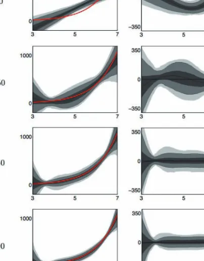
![Figure 4.14 below, plots the densities of both the classical indirect inference estimator (left) and the SNPII estimator (right) of the production function f along the capital dimension k t ∈ [80, 120] (at fixed steady-state TFP level of z ss = 0)](https://thumb-us.123doks.com/thumbv2/123dok_us/9460603.2820586/122.892.209.684.600.757/densities-classical-indirect-inference-estimator-estimator-production-dimension.webp)
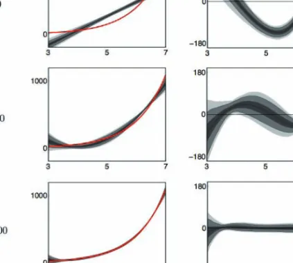
![Figure 4.15: Densities of standard II estimator (left) and SNPII estimator (right) of f along z ∈ [−1, 1] for fixed k ss = 100 and T = 200](https://thumb-us.123doks.com/thumbv2/123dok_us/9460603.2820586/123.892.209.682.299.455/figure-densities-standard-estimator-snpii-estimator-right-fixed.webp)
