Modeling Financial Contagion Using Mutually Exciting Jump Processes

NBER WORKING PAPER SERIES

MODELING FINANCIAL CONTAGION USING MUTUALLY EXCITING JUMP

PROCESSES

Yacine Aït-Sahalia

Julio Cacho-Diaz

Roger J.A. Laeven

Working Paper 15850

http://www.nber.org/papers/w15850

NATIONAL BUREAU OF ECONOMIC RESEARCH

1050 Massachusetts Avenue

Cambridge, MA 02138

March 2010

We are grateful to seminar and conference participants at Cornell, Princeton, Tilburg, Toulouse, City

University of London, University of Melbourne, University of Technology Sydney, the AFMATH

Conference in Brussels, the Cambridge-Princeton Conference and the TCF Workshop on Lessons

from the Credit Crisis, and in particular to Kenneth Lindsay, for their comments and suggestions. This

research was funded in part by the NSF under grant SES-0850533 (Aït-Sahalia) and by the NWO under

grants Veni-2006 and Vidi-2009 (Laeven). Matlab code to implement the estimation procedure developed

in this paper is available from the authors upon request. The views expressed herein are those of the

authors and do not necessarily reflect the views of the National Bureau of Economic Research.

NBER working papers are circulated for discussion and comment purposes. They have not been

peer-reviewed or been subject to the review by the NBER Board of Directors that accompanies official

NBER publications.

© 2010 by Yacine Aït-Sahalia, Julio Cacho-Diaz, and Roger J.A. Laeven. All rights reserved. Short

sections of text, not to exceed two paragraphs, may be quoted without explicit permission provided

Modeling Financial Contagion Using Mutually Exciting Jump Processes

Yacine Aït-Sahalia, Julio Cacho-Diaz, and Roger J.A. Laeven

NBER Working Paper No. 15850

March 2010

JEL No. C13,C32,G01,G15

ABSTRACT

Adverse shocks to stock markets propagate across the world, with a jump in one region of the world

seemingly causing an increase in the likelihood of a different jump in another region of the world.

To capture this effect mathematically, we introduce a model for asset return dynamics with a drift

component, a volatility component and mutually exciting jumps known as Hawkes processes. In the

model, a jump in one region of the world or one segment of the market increases the intensity of jumps

occurring both in the same region (self-excitation) as well as in other regions (cross-excitation). The

model generates the type of jump clustering that is observed empirically. Jump intensities then mean-revert

until the next jump. We develop and implement an estimation procedure for this model. Our estimates

provide evidence for self-excitation both in the US market as well as in other world markets. Furthermore,

we find that US jumps tend to get reflected quickly in most other markets, while statistical evidence

for the reverse transmission is much less pronounced. Implications of the model for measuring market

stress, risk management and optimal portfolio choise are also investigated.

Yacine Aït-Sahalia

Department of Economics

Fisher Hall

Princeton University

Princeton, NJ 08544-1021

and NBER

[email protected]

Julio Cacho-Diaz

Bendheim Center for Finance

26 Prospect Ave

Princeton, NJ 08540

[email protected]

Roger J.A. Laeven

Dept. of Econometrics and Operations Research

PO Box 90153

5000 LE Tilburg, The Netherlands

[email protected]

Figure 1: Mutual Excitation: Example I. This figure plots the cascade of declines in international equity markets experienced between February 26, 2007 and March 1, 2007 in the US; Latin America (LA); Developed European countries (EU); China; and Developed countries in the Pacific. Data are hourly. Source: MSCI MXRT international equity indices on Bloomberg.

1.

Introduction

Asset market crashes are very unlikely to occur under standard Brownian-driven statistical models, at least with volatility variables calibrated to realistic values. Even more unlikely would be crashes that happen in not just one, but multiple markets around the world at nearly the same time. And, even more unlikely would be further large price moves that happen in close succession over the following days, like earthquake aftershocks. Yet, despite the predictions of standard models, recurring crises happen every decade or so, with sufficient ferocity to overwhelm the statistical assumptions embedded in traditional models used for trading, portfolio management and derivative pricing. These crises seldom have discernible economic causes or warnings, and they tend to propagate across the world with little regard for economic fundamentals in the affected markets.

Of course, jump processes can be employed to capture the large moves in asset markets that continuous models are unable to generate. But the interplay between the various jump terms across markets and over time is not trivial, and standard jump specifications are unable to replicate those patterns. Indeed, adverse shocks to asset markets in one economic sector or region of the world seem to increase the probability of observing successive adverse shocks, not only in the market originally affected but also in other markets. Figures 1 and 2 illustrate two such recent examples, which took place in February 2007 and October 2008, respectively. Figure 1 describes the aftermath of a sharp

Figure 2: Mutual Excitation: Example II. Thisfigure plots the cascade of declines in international equity markets experienced between October 3, 2008 and October 10, 2008 in the US; Latin America (LA); UK; Developed European countries (EU); and Developed countries in the Pacific. Data are hourly. Source: MSCI MXRT international equity indices on Bloomberg.

decline that originated in the Chinese stock market. Even though this drop was perhaps not the only information that caused the European and US markets to fall —there was some concomitant macroeconomic news on durable goods in the US as well— its effect was felt in other markets in the form of a major downfall that by far exceeded the typical market reaction to macroeconomic news releases. Figure 2 shows what happened on and in the few days that followed October 3, 2008, when the prospects of a $700 billion bailout of the US financial sector were assessed in markets around the world. The figure shows that foreign markets followed the initial US drop in value by dropping in turn and that successive large price moves were then recorded over a period of days. More generally, when observed over a longer time period, as in Figure 3, where we plot daily stock index returns in six world regions, extreme moves tend to appear in clusters, both in time (horizontally) and in space (vertically).

These figures illustrate two key aspects of asset price jumps that we will model: they are clustered in time, and they tend to contaminate cross-sectionally to other regions. Jump clustering in time is a strong effect in the data. For example, from mid-September to mid-November 2008, the US stock market jumped by more than 5% on eight separate days. In the post-World War II era, jumps of magnitude greater than 5% of either sign have only happened on sixteen other days.

−0.2 0 0.2 US −0.2 0 0.2 UK −0.2 0 0.2 EU −0.2 0 0.2 JA −0.2 0 0.2 ASEM 1980 1985 1990 1995 2000 2005 −0.2 0 0.2 LA

Figure 3: Stock Index Returns in the Six World Regions. Thisfigure plots the log-returns of daily MSCI international equity index data. We consider six series: US; UK; Developed countries Europe (EU); Japan (JA); Emerging markets Asia (ASEM); and Latin America (LA). Sample period US, UK, EU and JA: January 1, 1980 to December 31, 2008; sample period ASEM: January 1, 1988 to December 31, 2008; sample period LA: January 29, 1988 to December 31, 2008. These series are the basis for our empirical analysis contained in Section 5. Descriptive statistics are in Table 1.

And intra-day fluctuations were even more pronounced: during the same two months, the range of intraday returns exceeded 10% during fourteen days. Cross-sectionally, the example in Figure 1 is one of the few cases in which the US stock market is affected by a non-US stock market jump. Usually, stock markets around the world appear to take their cues from the US market. A more typical situation is therefore that illustrated in Figure 2 where US news and market events lead successive market moves elsewhere around the world. As becomes apparent from inspection of the

figures, the shocks do not occur simultaneously, especially when viewed at intradaily frequencies. It takes some time for the transmission, if at all, to take place.1

In fact, what characterizes a crisis from the point of view of the time series properties of observed returns is typically not the initial jump, which is often limited in scope and in many cases could easily be absorbed, but the amplification that takes place subsequently over hours or days, and the fact that other markets become affected as well.2 _{To the best of our knowledge, existing time series} 1_{Differences in time zones and trading hours require careful consideration; our treatment of the data is discussed}

later in the paper.

2

There is lively debate in the literature regarding the meaning to give to the term “financial contagion,” whether it should be distinguished from spillovers, etc.: see e.g., Forbes and Rigobon (2002) for a discussion. Without taking sides in that debate, we use the term “financial contagion” throughout the paper to mean both the cross-region

models used to represent financial crises are not able to generate all these features, dynamic and cross-sectional, together.

To model this type of financial propagation, we need to leave the widely applied class of Lévy jumps, which is the usual class of driving processes employed in the literature. Lévy processes, such as the compound Poisson process, have independent increments: as a result, they do not allow for any type of serial dependence, whence propagation of jumps over time as well as propagation of jumps across markets are key components we wish to capture. So, in this paper, we employ a model for asset return dynamics that captures the cross-sectional and serial dependence observed across stock markets around the world. Mutually exciting jump processes, known as Hawkes processes, are natural candidates for modeling this “contagion” phenomenon mathematically.3 Basically, in a Hawkes process, a jump somewhere raises the probability of future jumps both in the same region and elsewhere. Jumps in asset returns therefore “self-excite” both in space and in time. In order for the asset returns process to be stationary, we then make the degrees of excitation of the various jumps, or jump intensities, mean revert until the next jump.

These jumps, by virtue of their self- and cross-excitation, introduce a feedback element. This aspect of the model can be thought of as playing the same role for jumps as ARCH does for volatility (see Engle (1982)). Namely, the ARCH model introduces feedback from returns to volatility and back: large returns lead to large volatilities which then make it more likely to observe large returns. In the absence of further excitation, volatility then reverts to its steady state level. Here, similarly, jumps lead to larger jump intensities, which then make it more likely to observe further jumps. In the absence of further excitation, jump intensities then revert to their steady state level.

Existing applications of Hawkes processes have typically employed them as pure point processes. As a result, the paths of the variables of interest will typically be piecewise constant, which is appropriate in many settings. Here, however, we wish to model asset prices. While our focus is on the return dynamics in times of crisis, we also wish to provide a model in which asset prices move normally and financial crises are rare. We will therefore not consider Hawkes processes on their own, but rather include them on top of the usual asset price components consisting of a drift or expected return, and a continuous or volatility component.

The paper makes two separate contributions. First, we propose a model consisting of a mutually exciting jump component added to a continuous Brownian component with stochastic volatility, as well as a drift term, which we refer to as a Hawkes jump-diffusion model by analogy with

transmission of shocks and the increase in the likelihood of successive shocks over time in the affected countries following an initial shock. While contagion in this broad sense can take place both during “good” times as well as during crisis times, the contagion phenomenon is more prevalent during crisis times.

3_{Hawkes processes were originally proposed as mathematical models to represent the transmission of contagious}

diseases in epidemiology. They have also found applications in neurophysiology and in the modeling of earthquake occurrences (see, e.g., Brillinger (1988) and Ogata and Akaike (1982)). In market microstructure, Bowsher (2007) employs them to jointly model transaction times and price changes at high frequency. Self-exciting models are now also being employed to model joint defaults in portfolios of credit derivatives; see e.g., Azizpour and Giesecke (2008). Hawkes processes have also been proposed in the literature on social interactions to model the “viral propagation” of some phenomena, such as the viewing of YouTube videos (see Crane and Sornette (2008).)

the Poissonian jump-diffusion model familiar to financial economists since Merton (1976). In the model, mutually exciting jumps are there to capture crises, while the remaining components are there to represent the evolution of the asset returns in normal times. Some important financial implications of the model we propose are investigated. Second, we develop and implement an estimation procedure for this model. Our estimation procedure is based on the generalized method of moments (GMM) using integrated moments of the model, which we derive in closed-form. This closed-form feature has some important advantages: it means, among other aspects, that we can deal with multivariate models and that the estimation is sufficiently fast to conduct an extensive Monte Carlo study to test its accuracy.4,5

When Hawkes processes are considered to model credit defaults, unlike our setting, the jump events in credit risk (defaults) are directly observable from the data. Here, due to the fact that neither the stochastic volatilities nor the jumps and jump intensities are directly observable, the corresponding inference problem we face is particularly challenging, and we develop an estimation procedure which explicitly accounts for the latency of part of the state vector. In brief, we do this by first computing the conditional moments using the full state vector: asset returns, stochastic volatilities, jumps and jump intensities; then conditioning down by taking expected values over

the latent state variables: volatilities, jumps and jump intensities. This results in expressions

that depend only upon theobservable state variables, namely the asset returns, but involve all the parameters of the model, including those driving the latent state variables.

We estimate our model using international stock index returns for six world regions. The empirical analysis indicates that both the US market as well as other markets strongly self-excite over time. Cross-sectionally, we find that US jumps tend to get reflected quickly in most other markets, while statistical evidence for the reverse transmission is much less pronounced.

As a model for asset prices that explicitly accounts for crises, our model is decidedly reduced-form. As such, it cannot explain the source(s) of the contagion that is observed in the data in times of crises, or get at the channels of transmission of that contagion, whether they are trade linkages,

financial linkages, financial constraints, outflows of capital, herding behaviors, the fragility of the system, lack of coordinated responses, etc. In all likelihood, all are important to different degrees 4_{The study of multivariate asset return models with jumps has recently seen a lot of activity. For example, Ang}

and Chen (2002) and Das and Uppal (2004) who study a Poisson-driven jump-diffusion model (a multivariate version of the Merton (1976) model). Ang and Chen (2002)find empirically that it fails to capture persistence of covariance dynamics in the data and captures almost no asymmetric correlation effects. Interesting to note is that none of the models considered in Ang and Chen (2002), which in addition to the jump-diffusion model include an asymmetric GARCH model, a regime-switching Gaussian model and a regime-switching GARCH model, completely explains the extent of observed asymmetries in correlation. Hawkes jump-diffusion models of the type that we study exhibit both persistence of co-variability and asymmetric co-variability and are therefore expected to outperform the simpler Poisson-driven jump-diffusion model. And, while the Poisson-driven jump-diffusion model studied by Ang and Chen (2002) and Das and Uppal (2004) captures only systemic jump risk, the jump risk model we propose captures both systemic jump risk and idiosyncratic jump risk.

5

In a univariate setting, Maheu and McCurdy (2004) and Yu (2004) provide clear evidence for jump clustering, supporting self-exciting jump models. Yu (2004) derives unconditional moments and autocovariances for the jump model proposed by Knight and Satchell (1998), which is of a different type than the univariate version of the mutually exciting model we study.

at different times in different crises, and there is an important literature, both theoretical and empirical, on these various mechanisms.6 Our model is merely a framework to quantify the nature and extent of the observed contagion, not an attempt at isolating the transmission mechanism(s). But, once estimated on the data, this reduced-form model can be employed as a description of the process driving the asset returns, notably their risk. In the Merton tradition, such reduced-form models are classically employed in finance for derivative pricing, portfolio choice or risk manage-ment, among others. In this context, the model is amenable to at least four important financial applications.

First, we discuss how the mutually exciting jump intensities of the model can be filtered out of the observed asset returns, and propose the resulting time series as a measure of market stress in lieu perhaps of volatility-based measurements such as the volatility index (VIX) which aggregates together both diffusive and jump risks. A second application of the model consists in quantifying the magnitude of the tails of asset returns. We evaluate the joint tails over the typical ten-day horizon that is employed in Value-at-Risk (VaR) calculations, and compute the systemic risk inherent in multiple assets jumping together in the same time period, comparing in particular the prediction of Poissonian jump-diffusions vs. Hawkes jump-diffusions. We find that most of the autocorrelation and cross-correlation patterns due to the mutually exciting component of the model tend to be important but die out after a few days, making the model ideally suited for this purpose. Third, it is possible to derive the optimal composition of an investor’s portfolio which is subject to continuous Brownian moves and mutually exciting jumps. Evidently, controlling exposure to jumps should be done on the basis of the most realistic model for correlated shocks. This motivates the study of more subtle forms of propagation in the form not just of simultaneous jumps within or across sectors, but rather in the form of a jump in one sector causing an increase in the likelihood that a different jump will occur in another sector.7 Finally, in terms of contingent claim pricing, we note that our model can be restricted to fit the rich class of affine jump-diffusion models, in their generalized version allowing for multiple jump types defined in Appendix B of Duffie et al. (2000). An affine special case of our model would therefore share in the tractable pricing implementation that results from an affine structure.

The rest of this paper is organized as follows: In Section 2, we present the model of asset returns, and discuss some of its properties. In Section 3, we develop our estimation procedure. In Section 4, 6_{See, e.g., Calvo and Mendoza (2000), Chang and Velasco (2001), Caramazza et al. (2004), Dornbusch et al. (2000),}

Dungey and Gonzalez-Hermosillo (2005), Dungey and Martin (2007), Eichengreen et al. (1996), Fry et al. (2009), Gerlach and Smets (1995), Rigobon (2003), Glick and Rose (1999), Kaminsky and Reinhart (1998), Kaminsky and Reinhart (2000), Kodres and Pritsker (2002), Krugman (1979), Nikitin and Smith (2008), Obstfeld (1996), Pavlova and Rigobon (2008) and Rijckeghem and Weder (2001).

7_{Other papers have studied the impact of time-varying correlations and jumps on portfolio choice in a framework}

without mutual excitation: Ang and Bekaert (2002) consider a regime-switching model, consisting of one regime with low correlations and low volatilities and one regime with higher correlations, higher volatilities and lower conditional means. They find that the existence of a higher volatility bear market regime does not nullify the benefits of international diversification, as long as the investor dynamically rebalances his portfolio. Das and Uppal (2004)find empirically that the loss reduction in diversification due to transmission across equity markets is not substantial. Aït-Sahalia et al. (2009) derive a closed-from solution to the portfolio choice problem with standard systematic, not mutually exciting, jumps across asset returns.

we study thefinite sample behavior of our estimators on the basis of a Monte Carlo study. Section 5 contains the empirical analysis. In Section 6, we investigate some implications of our model and its financial applications. Conclusions are in Section 7.

2.

Asset Return Dynamics

In our model, asset prices are subject to Brownian volatility as well as jumps. Relative to the classical jump-diffusion model infinance, which originated in Merton (1976), we allow the jumps to be mutually exciting in the fashion of Hawkes (1971a) as a means of capturing the contagion phenomenon: that is, a jump somewhere raises the likelihood of getting a jump elsewhere in the near future.

2.1.

Jump Dynamics: Mutually Exciting Processes

Hawkes (1971a) (see also Hawkes (1971b), Hawkes and Oakes (1974) and Oakes (1975)) introduced mutually exciting processes, which are special cases of path-dependent point processes. The inten-sities of a multivariate mutually exciting process depend on the paths of the point process; hence, the jump intensities are themselves stochastic processes and will be part of the state vector. The couple consisting of the jump process and its intensity remains a Markov process.

The jump intensities ramp up in response to jumps in one of the marginal point processes. We considerm point processes Ni,t,i= 1, . . . , m. In our application, there will be one such jump processNi,t for each of themregions of the world that we study. Of course, alternative breakdowns of the sample are possible, isolating sectors of the economy, for instance.

Similar to the familiar Poisson process, the Hawkes process is defined by its intensity process

λi,t which describes the Ft−conditional mean jump rate per unit of time, namely

⎧ ⎪ ⎨ ⎪ ⎩

P[Ni,t+∆−Ni,t = 0|Ft] = 1−λi,t∆+o(∆)

P[Ni,t+∆−Ni,t = 1|Ft] =λi,t∆+o(∆)

P[Ni,t+∆−Ni,t >1|Ft] =o(∆)

(2.1)

but instead of being constant the jump intensities follow the dynamics

λi,t =λi,∞+ m X j=1 Z t −∞ gi,j(t−s)dNj,s, i= 1, . . . , m. (2.2)

In other words, each previous jumpdNj,s, s∈(−∞, t), j= 1, . . . , m,raises the jump intensitiesλi,t. Taken jointly,(N, λ)is a Markov process. The distribution of the jump processesNj,sis determined by that of the intensities λj,s. Each compensated process Ni,t −

Rt

−∞λi,sds is a local martingale.

Hawkes processes are related to, but essentially different from, doubly stochastic Poisson (or Cox) processes: In a doubly stochastic Poisson process, the jump intensities are also stationary stochastic processes but the conditioning σ-algebra in (2.1) is _{Ni,s(s ≤ t) : λi,s(−∞ < s < ∞)}, i.e., the

path of λi,t is not affected by the path of Ni,t; see e.g., Karr (1991) for further details on doubly stochastic Poisson processes.

We assume that in (2.2) the constant parameters λi,∞ ≥ 0 for all i = 1, . . . , m, that the

real-valued functions gi,j(u) ≥ 0 for all u ≥ 0 and for all i, j = 1, . . . , m. Notice that λi,∞, gi,j being non-negative for alli, j= 1, . . . , mensures the non-negativity of the intensity processes with probability one.

Let Λ_∞ denote them_×1 vector with componentsλi,_∞ and Γ:=R₀∞Gudu them×m matrix whereGu is the matrix with elementsgi,j(u)’s. Letλi :=E[λi,t]denote the unconditional expected jump intensity, andΛ them_×1vector with components λi.Since from (2.1),E[dNi,s] =λids,we see that λi =λi,∞+ m X j=1 λj Z t −∞ gi,j(t−s)ds=λi,∞+ m X j=1 µZ ∞ 0 gi,j(u)du ¶ λj, (2.3)

or in vector formΛ=Λ_∞+Γ_·Λ.ThereforeΛ= (I₋Γ)−1Λ_∞, whereI is the identity matrix, and we assume that all the elements of Λ are positive and finite. This will ensure stationarity of the model.

2.2.

Full Dynamics: Mutually Exciting Jump-Di

ff

usion

The mutually exciting jump process constitutes only part of our model of asset returns. We assume that asset log-returns follow the semimartingale dynamics

dXi,t =μidt+σidWi,t+Zi,tdNi,t, i= 1, . . . , m, (2.4)

which consists of a drift term, a volatility term, and mutually exciting jumps. Here, Wt :=

[W1,t, . . . , Wm,t]0is anm-dimensional vector of standard Brownian motions with constant correlation coefficientsρi,j, i, j = 1, ..., m,Z := [Z1, . . . , Zm]0 is the vector of jump sizes, cross-sectionally and serially independently distributed with lawsFZi supported on(−∞,∞), andNt:= [N1,t, . . . , Nm,t]0

is the vector of Hawkes processes just described. Throughout, all dynamics are with respect to the objective probability measure and not to an equivalent martingale measure. Zi may be replaced by log³1 + ˜Zi

´

so that the discontinuous part in the differential of the stochastic exponential

eXi,t _{becomes Z}˜

ieXi,tdNi,t. For notational convenience we writeZi rather thanlog

³ 1 + ˜Zi

´

. We will leave the distribution of jump sizes essentially unrestricted, so asymmetries such as negative jumps (crashes) being more likely than positive jumps (booms), can be built into the jump size distributions.

In the base model (2.4), the quantities μi and σi are constant parameters. In this case we assume that Σ, the m_×m-dimensional variance-covariance matrix of the risk coming from the continuous part of the model, with elements Σi,j = ρi,jσiσj, is a non-singular matrix. We always assume that the vector of Brownian motionsW, the vector of jump sizes Z and the vector of jump processes N are mutually independent.

In an extension of the model (2.4), we allow for stochastic volatility:

dXi,t=μidt+

p

Vi,tdWi,tX+Zi,tdNi,t, (2.5)

where the instantaneous variance follows the Heston (1993) model

dVi,t =κi(θi−Vi,t)dt+ηi

p

Vi,tdWi,tV, (2.6)

with κi, θi, ηi constant parameters. Model (2.4) corresponds to the special case where the initial value isVi,0=θi andηi = 0.Note thatVi,t is a local variance rather than a local standard deviation; while keeping this in mind we will refer toVi,t as the stochastic volatility variable. Vi,t follows the square root process of Feller (1951) and is bounded below by zero. The boundary value zero cannot be achieved as long as Feller’s condition,2κiθi ≥ηi2, is satisfied.

The extended model allows for correlations among the individual Brownian motions driving equations (2.6) as well as between the individual Brownian motions driving equations (2.5) and (2.6), thereby capturing a potential leverage effect. But in the presence of systematic jumps, the Brownian correlation, even if it increases, will not play a major role: in times of crisis, jumps swamp everything else.8

Our estimation procedure can cover general stochastic volatility specifications, and we show below how to derive closed-form expressions for observable moments of the log-returns. But we need to settle on a specific model with interpretable parameters to do the actual parametric estimation, and for this purpose we assume that the volatility follows the model (2.6).

Our model, with mutually exciting jump processes added to a continuous Brownian component with (possibly stochastic) volatility as well as a drift, will be referred to as aHawkes jump-diffusion. Hawkes jump-diffusion processes will generate observed time-varying correlations and maximal correlations around crisis times, due to the systematic jumps. Isolating a change in the structure of the Brownian variance-covariance matrix Σ becomes difficult in this context, because linear correlation measures weigh equally all returns; as a result, they will tend to average out any contagion that happens over a limited number of days among the comparatively large number of days where no jumps occur.9 _{Similarly, the observed clustering of extreme returns is generated} by Hawkes jump-diffusion processes in a different manner from pure stochastic volatility models where periods of high volatility can also lead to clusters of larger absolute returns, although not of a magnitude and rate of occurrence compatible with what is actually observed in the data.

8_{The linear correlation measure of dependence is not an appropriate measure for the type offinancial propagation}

observed in crises (see Bae et al. (2003) and Longin and Solnik (2001) for a discussion). Abandoning the correlation framework, Bae et al. (2003) use a multinomial logistic regression model to model and evaluate joint occurrences of large absolute value returns.

9

Analyzing correlation structures between asset returns, Goetzmann et al. (2005)find that (linear) correlations across world markets vary significantly over time. Evidence from capital markets history suggests that periods of poor market performance are associated with high correlations. They find that average correlations went up and reached a peak in the 1930’s (Great Depression) that has been unequaled until the modern era. Bekaert and Harvey (1995) and Bekaert and Harvey (2000) provide evidence that market integration and financial liberalization change the comovement of emerging markets stock returns with the global market factor.

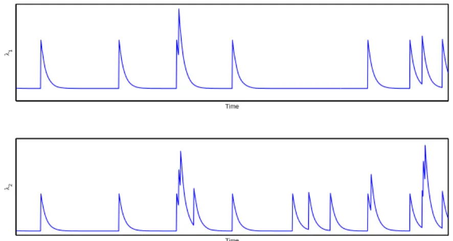
Time λ1

Time λ2

Figure 4: Jump Intensity Processes: A Sample Path. Thisfigure plots a sample path of the intensity processes (λ1,t, λ2,t) generated by a bivariate mutually exciting Hawkes process with exponential

decay (see Section 2.3).

2.3.

Mean Reversion in Jump Intensities

The tractability of the jump part of our model, and hence the possibility of estimating it, depends on the parameterization of the intensity processes λi,t. A special case of interest occurs when

gi,j(t−s) =βi,je−αi(t−s), s < t, i, j = 1, . . . , m, (2.7) withαi>0,βi,j ≥0for alli, j= 1, . . . , m. In this case, a jump in asset prices causes the intensities to jump up, and then the intensity decays exponentially back: λi,t jumps byβi,j whenever a shock in sector j occurs, and then decays back towards a level λi,∞ at speed αi. Figure 4 illustrates a

sample path of the jump intensity processes in the bivariate mutually exciting case. Asset return dynamics of equity markets that are highly interrelated may exhibit jumps that take place almost simultaneously. In our model this corresponds to the case in which mutual excitation is very severe (largeβi,j,i6=j).

With this model, the Γ matrix is given by

Γ= ⎛ ⎜ ⎝ β11 α1 · · · β1m α1 .. . . .. ... βm1 αm · · · βmm αm ⎞ ⎟ ⎠. (2.8)

Under exponential decay (2.7), each jump intensity has the mean-reverting dynamics

dλi,t=αi(λi,∞−λi,t)dt+ m

X

j=1

Other specifications of the intensity process may also be considered and it is possible to obtain the covariance density matrix and spectral density for general gi,j functions. In even more general specifications, the intensity may depend not only on the amount of time elapsed since a jump event but also on the size of past jump events.

The jump part of the model is able to generate the two features we are after: First, jump activity is variable over time, with many (of the few) jumps typically being concentrated in short periods of time; this is jump clustering. Second, adverse shocks propagate across the world in a contagious way, with adverse events in one region of the world seemingly increasing the likelihood of shocks in other regions of the world; this is jump propagation. Under exponential decay, the element-by-element Laplace transformV_N∗(s) of the covariance density matrixVN(τ) is given by

V_N∗(s) = (I₋G∗(s))−1¡G∗(s)Diag(Λ) +βV_N∗ 0_{α_}/_{α+s_}¢, (2.10) withG(τ)them_×m-matrix given by

G(τ) = ⎛ ⎜ ⎝ β11e−α1τ · · · β1me−α1τ .. . . .. ... βm1e−αmτ · · · βmme−αmτ ⎞ ⎟ ⎠, (2.11)

andG∗_{(s) its element-by-element Laplace transform. The indices of{a} and{a+s} correspond to}

the element-by-element indices ofβ.

With stochastic volatilities and stochastic jump intensities added to the state vector, our model can be restricted to be part of the class of generalized affine jump-diffusion processes. To see this, consider a generalized affine jump-diffusion A in a state space D _{⊂ R}3×m, defined as a strong solution to the stochastic differential equation

dAt=μA(At)dt+σA(At)dWtA+ m

X

j=1

dJj,t, (2.12)

where μA:D_→R3×m, σA:D_→R(3×m)×(3×m),WA is a Brownian motion in_R3×m, and Ji, i=

1, . . . , m, are pure jump processes with jump intensities λA_i,t =λA_i (At), for some λAi :D→ [0,∞), and with fixed jump size distributions on _R3×m. It is possible to restrict a process A of the form (2.12) to be affine, by considering the special case whereμA, σAσA0 and λA_t are affine on D. Then our Hawkes jump-diffusion model with exponential decay can be restricted to be affine by setting

At= [Xt, Vt, λt]0 with the corresponding μA, σAσA0 andλAt being affine.

2.4.

Jump Size Distribution

We have noted that the analysis can proceed without assumptions on the distribution of the jump magnitudes, and in fact, we will provide expressions for the moments of the process as functions of the generic moments of the jump size Zt, which we denote M[Z, k] := E

£

Z_tk¤. In order to estimate a specific parametric model, however, we need to parameterize these moments to reduce

the dimensionality of the parameter space, given that the distribution of jumps offinite activity is difficult to pin down since large jumps are by nature rare.

For this purpose, we will assume thatZi is a scalar random variable with cumulative probability distribution FZi(x) = ( pie−γi,1(−x), −∞< x≤0; pi+ (1−pi)(1−e−γi,2x), 0< x <∞; (2.13) whereγi,1, γi,2 >0 and 0≤pi ≤1,i= 1, . . . , m. The corresponding density is

fZi(x) =

(

piγi,1e−γi,1(−x), −∞< x≤0;

(1₋pi)γi,2e−γi,2x, 0< x <∞.

(2.14) One easily verifies that

E h Z_iki= (₋1)kk!pi γ_i,k₁ + k! (1₋pi) γ_i,k₂ , k= 1,2, . . . . (2.15)

This jump size distribution is also used by Kou (2002) in the context of option pricing.

In our empirical study below we use equity index data. As such, our analysis does not suffer from survivorship bias. However, survivorship bias, when present (for example, when individual stock returns are used), can easily be dealt with in this model. Explicitly modeling the survival and death process involves introducing a point mass at Zi =−∞ in the distribution of the jump size for log-returns.

3.

Estimation Procedure

Neither the point processesNi,t and the intensity processes λi,t, nor the stochastic volatilitiesVi,t,

i= 1, . . . , m, are directly observable. Instead, what is observed are asset prices, hence log-returns

Xi,t. It turns out that we can derive explicit expressions for the moments of the log-returns that are implied by the model, as a function only of the observable state variables, in effect integrating out the unobservable state variables. We will therefore develop a GMM-based estimation procedure.

3.1.

Explicit Expressions for the Moments: Markov In

fi

nitesimal Generator

The key to the estimation procedure is the availability in closed-form of the main moments for the model. Having the moment conditions in closed-form means that the effort involved in minimizing the GMM criterion function becomes minimal, despite the number of parameters and moment functions. The moment conditions that we will use to carry out GMM estimation of the model are:

⎧ ⎪ ⎪ ⎪ ⎨ ⎪ ⎪ ⎪ ⎩ E[∆Xi,t] E[(∆Xi,t−E[∆Xi,t])r], r = 2, . . . ,4 E[∆Xi,t∆Xj,t−E[∆Xi,t]E[∆Xj,t]], i6=j E[∆Xi,t+τ∆Xj,t−E[∆Xi,t]E[∆Xj,t]], τ >0. (3.1)

As we will see, the reason for using these moment functions is two-fold. First, they are “natural” in the sense of being easily interpretable: variance, kurtosis, autocovariances. Second, and more importantly, each moment function plays a specific role in identifying parts of the model.

Throughout the analysis, we use unconditional moments as opposed to conditional moments. To compute the unconditional moments, wefirst compute the conditional moments using the full state vector: asset returns, stochastic volatilities, jumps and jump intensities. Next, we take expected values, integrating out the latent state variables: volatilities, jumps and jump intensities. Doing so, we obtain expressions that depend only upon the observable state variables: asset returns. These expressions, however, contain all the parameters of the model, including those related to the latent state variables.

To compute the conditional moments, we use the explicit expression of the generator of the Markov process (2.4) or (2.5)-(2.6) driven by the processes(W, N, λ).Specifically, the computation of the moment functions reduces to the evaluations of conditional expectations of functions of the form f(y1, y0, δ) where y1 and y0 denote log-returns separated by some function of the sampling

intervalδ.We assume that sampling is equidistant in time. We need to evaluate expressions of the form _EY1,Y0[f(Y1, Y0,∆)]. The dynamics of the system depends upon additional latent variables

which at the same instants we denote byξ1 = (v1, l1) and ξ0= (v0, l0), respectively, wherev is the

volatility and l the jump intensity. The standard infinitesimal generator _Ais the operator which, when applied to a function g(y1, y0, ξ1, ξ0, δ) in its domain, returns the functionA ·g given in full

generality by A ·g= ∂g ∂δ + m X i=1 μX_i ∂g ∂y1,i + m X i=1 μV_i ∂g ∂v1,i + m X i=1 μλ_i ∂g ∂l1,i (3.2) +1 2 m X i=1 m X j=1 σY Y_ij ∂ 2_g ∂y1,i∂y1,j +1 2 m X i=1 m X j=1 σ_ijY V ∂ 2_g ∂y1,i∂v1,j +1 2 m X i=1 m X j=1 σV V_ij ∂ 2_g ∂v1,i∂v1,j + m X i=1 l1,i Z zi {g(y1+zi, y0, v1, l1+βi, v0, l0, δ)−g(y1, y0, v1, l1, v0, l0, δ)}fZi(zi)dzi,

whereμX is the vector of expected log-returns,μV the vector of stochastic volatility drifts,μλ the vector of jump intensity drift,σY Y the variance-covariance matrix of log-returns,σY V the variance-covariance matrix of interactions between returns and volatilities, σV V the variance-covariance matrix of stochastic volatilities and finally βi = [βi,1, ..., βi,m]0 the vector of excitation parameters for theith jump term. In the case of the mean-reverting jump intensity model described in Section 2.3, we have μλ_i =αi(λi,∞−l1,i).

The usefulness of the infinitesimal generator for our purpose lies in the fact that

EY1,ξ1[g(Y1, Y0, ξ1, ξ0,∆)|Y0, ξ0] = exp (∆A)·g(Y0, Y0, ξ0, ξ0,0) = J X j=0 ∆j j! ¡ Aj·g¢(Y0, Y0, ξ0, ξ0,0) +Op ¡ ∆J+1¢, (3.3)

where subscripts in _EY1,ξ1 indicate the random variables that the expected value operates on, and

Aj·g is defined recursively by _Aj_·g=_{A ·}(_Aj−1_·g) for all j_≥1.As we will see in the theorems that follow, (3.2) and its iterates _Aj _{·g, hence the terms in (3.3), can be evaluated in closed-form} for the moment functions of interest given in (3.1). While the starting moment functionf(y1, y0, δ)

does not depend directly upon the latent variables(ξ1, ξ0),A ·f and successive iterates will, since

the coefficients _{μX, μV, μλ, σY Y, σY V, σV V, βi} will in general depend on the full state variables

[X, V, λ].

In other words, we can obtain the conditional expectation of g, using the full state vector including its unobservable components,_EY1,ξ1[g(Y1, Y0, ξ1, ξ0,∆)|Y0, ξ0].We then need to “condition

down” by integrating out the unobservable state variables in order to produce moment functions that can be fitted to the log-returns data. All the expectations are taken with respect to the law of the process at the true parameter values. From the law of iterated expectations, we have that

EY1,Y0,ξ1,ξ0[g(Y1, Y0, ξ1, ξ0,∆)] =EY1,Y0,ξ1,ξ0[EY1,ξ1[g(Y1, Y0, ξ1, ξ0,∆)|Y0, ξ0]] = J X j=0 ∆j j! EY0,ξ0 £¡ Aj ·g¢(Y0, Y0, ξ0, ξ0,0) ¤ +Op ¡ ∆J+1¢, (3.4)

so the last step in the necessary calculations will involve computing unconditional expectations with respect to the stationary law of the state variables.

3.2.

The Univariate Case

For ease of exposition, we first provide the expressions of these moments in the univariate case

m= 1.In this situation, we are looking at a single asset with stochastic volatility and jumps that self-excite, meaning that future jump intensities depend upon the history of their own past jumps:

⎧ ⎪ ⎨ ⎪ ⎩ dXt=μdt+√VtdWtX+ZtdNt dVt=κ(θ−Vt)dt+η √ VtdWtV dλt=α(λ∞−λt)dt+βdNt (3.5)

with_E£dW_tXdW_tV¤=:ρVdt andλ:=_E[λt] =αλ∞/(α−β).Note that classical compound Poisson

process jumps are obtained whenβ = 0andλ0 =λ∞.Then λt=λ∞=λat all t.

At this stage, we can leave the distribution of the jump size essentially unrestricted, and provide expressions as functions of the moments of the jump sizeZt,for which we write M[Z, k] :=E

£ Z_tk¤.

Our first main result states that:

by the following expressions E[∆Xt] = (μ+λM[Z,1])∆+o(∆2) E£(∆Xt−E[∆Xt])2 ¤ = (θ+λM[Z,2])∆+βλ(2α−β) 2(α₋β) M[Z,1] 2_∆2_+o(∆2₎ E£(∆Xt−E[∆Xt])3 ¤ =λM[Z,3]∆ +3 2 µ ηθρV +(2α−β)βλM[Z,1]M[Z,2] (α₋β) ¶ ∆2+o(∆2) E£(∆Xt−E[∆Xt])4 ¤ =λM[Z,4]∆+ µ 3θη2 2κ + 3θ 2_{+ 6θλM[Z,2]} + 3λ µ λ+(2α−β)β 2(α₋β) ¶ M[Z,2]2 + 2(2α−β)βλM[Z,1]M[Z,3] (α₋β) ¶ ∆2+o(∆2)

while the autocorrelation function of the process is given by

E[(∆Xt−E[∆Xt])(∆Xt+τ−E[∆Xt+τ])] =

βλ(2α₋β) 2(α₋β) e

−(α−β)τ_M[Z,1]2_∆2_+o(∆2₎

for all τ >0.

Intuitively, the identification of the parameters is achieved as follows: the higher order moments (3 and 4) isolate the jump parameters at the leading order, while the variance puts them on an equal footing with the diffusive parameters.10 _{The autocovariance isolates the jump parameters.} Indeed, if the model had no jump component, then from (3.5) with Zt ≡ 0, the law of iterated expectations implies that

E[(∆Xt) (∆Xt+τ)] =E[(∆Xt)E[(∆Xt+τ)|Ft+τ]] =E[(∆Xt) (μ∆)]

=_E[_E[(∆Xt)|Ft] (μ∆)] =μ2∆2 and so _E[(∆Xt−E[∆Xt])(∆Xt+τ−E[∆Xt+τ])] = 0.

Thus any autocovariance is due to the jump component. Further, if the jump component is Poissonian, then the increments would be independent and it is the self-excitation of the jumps that gives rise to the autocorrelation. Thus the observed autocovariance of the increments isolates the self-exciting component of the model.

As noted above, the model reduces to a Poissonian jump-diffusion if β = 0. Then we indeed 1 0_{We use regular moments as opposed to absolute moments. The use of absolute moments —especially absolute}

moments of order less than 1 (see Aït-Sahalia (2004))— may be considered in addition, especially for estimating parameters of the volatility process. Since we are mainly interested in the parameters of the jump process we have chosen to consider only regular moments in the interest of simplicity and parsimony.

have E[∆Xt] = (μ+λM[Z,1])∆+o(∆2) E£(∆Xt−E[∆Xt])2 ¤ = (θ+λM[Z,2])∆+o(∆2) E£(∆Xt−E[∆Xt])3 ¤ =λM[Z,3]∆+ 3 2ηθρ V_∆2_+o(∆2₎ E£(∆Xt−E[∆Xt])4 ¤ =λM[Z,4]∆+ 3 µ θη2 2κ + (θ+λM[Z,2]) 2 ¶ ∆2+o(∆2)

and the model does not generate any autocorrelation.

It is clear from the explicit expressions of these moments that there will be difficulty in practice identifying the stochastic volatility parameters: there are simply too many latent processes:Vt, Nt,

λt;while those are integrated out as part of the development of the unconditional moments, their corresponding parameters remain. So they are theoretically identified, but this identification can be tenuous in practice. This is an unavoidable consequence of the unobservability of those state variables. This will be especially so in the multivariate context where there are many potential correlation coefficients: between each asset’s log-return and all the volatilities, among the different asset log-returns and among the different volatilities. To avoid this problem, we will restrict some of the parameters to be identical, and identify only the level of the volatility.

3.3.

The Bivariate Case

We now turn to the bivariate case, m = 2. We consider the general case in the Appendix, but restrict attention here to the more tractable triangular excitation case, whereβ12 = 0, with

state-independent volatilities. That is, the base model is

⎧ ⎪ ⎪ ⎪ ⎨ ⎪ ⎪ ⎪ ⎩ dX1t=μ1dt+σ1dWt1+Z1tdN1t dX2t=μ2dt+σ2dWt2+Z2tdN2t dλ1t=α1(λ1∞−λ1t)dt+β11dN1t dλ2t=α2(λ2∞−λ2t)dt+β21dN1t+β22dN2t (3.6) with_E[dW_t1dW_t2] =:ρdt.

Theorem 2. For the bivariate model (3.6), the mean and variance of the log-returns are given in

closed-form up to order ∆2 by the following expressions

E[∆X1t] = (μ1+λ1M[Z1,1])∆+o(∆2)

and E£(∆X1t−E[∆X1t])2 ¤ =¡σ2₁+λ1M[Z1,2] ¢ ∆+(2α1−β11)β11λ1 2(α1−β11) M[Z1,1] 2_∆2_+o(∆2₎ E£(∆X2t−E[∆X2t])2 ¤ = (σ2 2+λ2M[Z2,2])∆+ µ β2 21(α21+(α1−β11)(α2−β22))λ1 2(α1−β11)(α2−β22)(α1+α2−β11−β22) + (2α2−β22)β22λ2 2(α2−β22) ´ M[Z2,1]2∆2+o ¡ ∆2¢ E[(∆X1t−E[∆X1t])(∆X2t−E[∆X2t])] =ρσ1σ2∆ +β21(α 2 1+(α1−β11)(α2−β22))λ1 2(α1−β11)(α1+α2−β11−β22) M[Z1,1]M[Z2,1]∆ 2_+o¡_∆2¢_.

As expected, the variance places the contributions from the diffusive and jump components of the model on the same level. However, the leading terms of the higher order moments isolate the jump component:

Theorem 3. The higher order moments of the bivariate model are given up to order ∆2 _{by the} following expressions: E£(∆X1t−E[∆X1t])3 ¤ =λ1M[Z1,3]∆+ 3(2α₂₍1_α−β11)β11λ1 1−β11) M[Z1,1]M[Z1,2]∆ 2_+o(∆2₎ E£(∆X2t−E[∆X2t])3 ¤ =λ2M[Z2,3]∆+ 3₂ ³ (2α2−β22)β22λ2 (α2−β22) + (α 2 1+(α1−β11)(α2−β22))λ1β221 (α1−β11)(α2−β22)(α1+α2−β11−β22) ¶ M[Z2,1]M[Z2,2]∆2+o(∆2) E£(∆X1t−E[∆X1t])2(∆X2t−E[∆X2t]) ¤ = β21(α 2 1+(α2−β22)(α1−β11))λ1 2(α1−β11)(α1+α2−β11−β22) ×M[Z1,2]M[Z2,1]∆2+o(∆2) E£(∆X1t−E[∆X1t])(∆X2t−E[∆X2t])2 ¤ = β21(α 2 1+(α2−β22)(α1−β11))λ1 2(α1−β11)(α1+α2−β11−β22) ×M[Z1,1]M[Z2,2]∆2+o(∆2) E£(∆X1t−E[∆X1t])4 ¤ =λ1M[Z1,4]∆+ ¡ 3σ₁4+ 6M[Z1,2]λ1σ12 +3M[Z1,2]2λ1(2α1(β11+λ1)−β11(β11+2λ1)) 2(α1−β11) + 2(2α1−β11)β11λ1 (α1−β11) M[Z1,1]M[Z1,3] ´ ∆2+o(∆2) E£(∆X2t−E[∆X2t])4 ¤ =λ2M[Z2,4]∆+ ¡ 3σ₁4+ 6M[Z2,2]λ2σ22 +3M[Z2,2]2(η22+β22λ2) + 4 (η22+ (β22−λ2)λ2)M[Z2,1]M[Z2,3])∆2+o(∆2).

The other contemporaneous cross-terms that are not listed above,

Eh(∆X1t−E[∆X1t])j(∆X2t−E[∆X2t])k

i ,

of orderj+k= 4,are of smaller orderO(∆2).

The expressions above depend upon expected values and variances of the jump intensities, which are given by λ1 :=E[λ1t] = _αα₁1₋λ1_β,∞₁₁ λ2 :=E[λ2t] = α1β21λ1,₍∞_α+α1α2λ2,∞−α2β11λ2,∞ 1−β11)(α2−β22) and η11:=E £ λ2 1t ¤ =λ2₁+ β211λ1 2(α1−β11) η22:=E£λ22t ¤ =λ2₂+ β222 λ2 2(α2−β22)+ (α2 1+(α2−β22)α1+β11(β22−α2))λ1β212 2(α1−β11)(α2−β22)(α1+α2−β11−β22) η12:=E[λ1tλ2t] =λ2λ1+_2(α (2α1−β11)β11β21λ1 1−β11)(α1+α2−β11−β22).

The final result provides the autocovariance function of the bivariate model:

Theorem 4. For the bivariate model (3.5), the autocovariances of the log-returns at lag τ >0, Ci,j(τ) :=E[(∆Xj,t−E[∆Xj,t])(∆Xi,t+τ−E[∆Xi,t+τ])],

are given in closed-form up to order ∆2 by the following expressions, which are driven by the

mutually exciting component of the model:

C1,1(τ) =e−τ(α1−β11)a11,1M[Z1,1]2∆2+o(∆2) C1,2(τ) =e−τ(α1−β11)a12,1M[Z1,1]M[Z2,1]∆2+o(∆2) C2,1(τ) = ¡ e−τ(α1−β11)_a 21,1+e−τ(α2−β22)a21,2 ¢ M[Z1,1]M[Z2,1]∆2+o(∆2) C2,2(τ) = ¡ e−τ(α1−β11)_a 22,1+e−τ(α2−β22)a22,2 ¢ M[Z2,1]2∆2+o(∆2) where a11,1= (2α₂₍1−_αβ₁₋11_β)₁₁β11₎λ1 a12,1= _2(α1−(2_βα₁₁1−₎₍β_α11₁₊)β_α11₂₋β21_β11λ1_−β22) a21,1= _2(α1−(2_β11α1₎₍−₋β_α11₁)₊β_α11₂β₊21_βλ₁₁1_−β22) a21,2= β21(α21−(α2−β22)2)λ1 (α1+α2−β11−β22)(α1−α2−β11+β22) a22,1= (2α1−β11)β11λ1β 2 21 2(α1−β11)(α1+α2−β11−β22)(−α1+α2+β11−β22) a22,2= (2α₂₍2−_αβ₂₋22_β)₂₂β22₎λ2 + ( α21−(α2−β22)2)λ1β212 2(α2−β22)(α1+α2−β11−β22)(α1−α2−β11+β22).

As in the univariate case, the diffusive component of the model generates no autocorrelation. Also, the autocorrelation structure is asymmetric, reflecting the fact that the excitation from jumps in sector 1 to jumps in sector 2 is not the same as that from jumps in sector 2 to jumps in sector 1.

3.4.

Interval-Based Moment Functions

GMM can be carried out using the instantaneous moments above, on short time intervals (daily). However, in order to improve accuracy and reduce the number of moment conditions to be used, we calculate in addition the unconditional interval-based moments (i, j= 1,2; 0_≤s1 < s2 < s3 < s4)

⎧ ⎪ ⎪ ⎪ ⎪ ⎪ ⎪ ⎪ ⎨ ⎪ ⎪ ⎪ ⎪ ⎪ ⎪ ⎪ ⎩ EhRs2 s1 dXi,t i E ∙_³R s2 s1 dXi,t−E hRs2 s1 dXi,t i´2¸ EhRs2 s1 dXi,t Rs2 s1 dXj,u−E hRs2 s1 dXi,t i EhRs2 s1 dXj,u ii , i₆=j EhRs4 s3 dXi,u Rs2 s1 dXj,t−E hRs4 s3 dXi,u i EhRs2 s1 dXj,t ii

which can be applied on time intervals of arbitrary lengths. We are also able to compute these integrated moment conditions in closed-form.

The explicit formulae we derive for the moment conditions are contained in the Appendix. The (lengthy) closed-form expressions for the integralsIτ

as for the derivatives of the moment conditions (needed to compute Ω; see (3.11) below) are not displayed in this paper to save space. These expressions are available in computer form from the authors upon request.

3.5.

Array of Autocovariances and Cross-Covariances

To implement GMM with these interval-based moment conditions, a choice has to be made on the “array” of autocovariances and covariances (i.e., the number of autocovariances and cross-covariances, and the length of the intervals of integration) to be used. Autocorrelograms and cross-correlograms of the data can be used as exploratory tools for determining the total length of the time period on which autocovariances and cross-covariances are to be considered.

Finding the “optimal” array of autocovariances and cross-covariances, striking a balance be-tween accuracy and computational feasibility, has been one of our objectives in an extensive Monte Carlo study, which we will present below. Also, in case the sampling interval ∆ that we use to compute the first four moments and the instantaneous autocovariances and cross-covariances is different from the sampling interval∆that we use to compute (lagged) autocovariances and cross-covariances, we use a varying number of observations for different elements in the GMM procedure and as such the scalarN needs to be replaced by a vector in the relevant places.

3.6.

GMM Estimation

Given the expressions for the moment functions above, we proceed to estimate the parameters of the model using standard GMM. LetYn∆:=Xn∆−X(n−1)∆,n= 1, . . . , N,∆>0, withN∆=T,

denote the log-returns on the interval [0, T] and let θ _∈ Θ denote our d-dimensional parameter vector. To estimateθwe consider a vector ofM moment conditionsh(y,∆, θ),M _≥d, continuously differentiable in θ. Let θ0 denote the true value ofθ and suppose that E[h(Yn∆,∆, θ0)] = 0.This

is the key requirement for consistency of the GMM estimator. The closed-form expressions for the moments derived above ensure that it will be satisfied, since we will use for each component of the vector h the difference between the corresponding sample moment of the log-returns and its closed-form expression derived under the model.

We assume that the log-returns are stationary, which is the case for our model under the parameter restrictions discussed above. LetgT(y,∆, θ) denote the sample average of h(yn∆,∆, θ),

that isgT(y,∆, θ) := _N1 PN_n=1h(yn∆,∆, θ).Then the GMM estimatorθˆT is the value ofθ∈Θthat minimizes the quadratic form

gT(y,∆, θ)0 WT gT(y,∆, θ), (3.7)

where WT is an M ×M positive definite weight matrix assumed to converge in probability to a positive definite limit W. The system is exactly identified if M =d, in which case the choice of

WT becomes irrelevant.

{h(Yn∆,∆, θ0)}∞n=−∞ is strictly stationary with mean zero and v-th autocovariance matrix Γv :=

E£h(Yn∆,∆, θ0) h(Y(n−v)∆,∆, θ0)0

¤

.Assuming that these autocovariances are absolutely summable (i.e., that the sequence of partial absolute sums has a finite limit), let S := P∞_v=−∞Γv. We note thatS is the asymptotic variance of the sample average of h(yn∆,∆, θ0):

S = lim N→∞N E £ gTN(Y,∆, θ0) gTN(Y,∆, θ0)0 ¤ . (3.8)

The optimal weight matrix turns out to be S−1. A non-negative definite estimator ofS is

ˆ ST = ˆΓ0,T + Xq v=1 µ 1₋ v q+ 1 ¶ ³ ˆ Γv,T+ ˆΓ0v,T ´ , (3.9) with ˆ Γv,T = 1 N XN n=v+1h(yn∆,∆, ˜ θ) h(y(n−v)∆,∆,θ˜)0. (3.10)

Here θ˜ is an initial consistent estimate of θ0, which can be obtained by minimizing (3.7) with

WT =I.

Under standard regularity conditions (see Hansen (1982)), √TN(ˆθ−θ0) converges in law to

N(0,Ω)where

Ω−1 :=∆−1D0W D(D0W SW D)−1D0W D, (3.11)

and D is the gradient of E[h(Yn∆,∆, θ)] with respect to θ0 evaluated at θ00. When WT is chosen optimally,W =S−1 _{and (3.11) reduces to Ω}−1 _=∆−1_D0_S−1_D.

3.7.

Testing for the Presence of Contagion

If desired, it is possible to test for the presence of contagion in the context of our model. Whether or not contagion occurs boils down here to testing the joint hypothesis that all the coefficients of mutual excitation βi,j’s are 0. We can further separate between testing for self- or time-series contagion: diagonal βi,i = 0 and testing for cross-sectional contagion: off-diagonal βi,j = 0, i6= j. Since the inference is based on standard GMM given the relevant moment functions, GMM-based testing tools apply to test these parameter restrictions. We will employ below for this purpose the

χ2 statistic that follows from (3.11).

4.

Finite Sample Behavior: A Monte Carlo Study

One major advantage of the proposed estimation method is that it is numerically tractable, so that large numbers of Monte Carlo simulations can be conducted to determine the finite sample distribution of the estimators. From the onset, one should be aware of the fact that one cannot expect degrees of accuracy similar or even close to what we are used to when estimating, e.g., a standard stochastic volatility model. By definition, extreme events occur infrequently and there is a positive probability that no jump occurs in any givenfinite time interval. When no jump occurs,

0.135 0.136 0.137 0.138 0.139 0.14 0.141 0.142 0.143 θ1/2 density 0 0.05 0.1 0.15 γ−1 density 0 0.5 1 1.5 2 2.5 3 λ∞ density 0 5 10 15 20 25 30 35 40 α density 0 5 10 15 20 25 30 35 40 β density 0 2 4 6 8 10 λ density

Figure 5: Monte Carlo Results: Univariate Case. This figure plots the empirical distribution functions of the parameter estimators for the univariate Hawkes jump-diffusion model, obtained from 5,000 simulated sample paths.

there is no identification whatsoever, while when few jumps occur identification is expected to be weak. This is a consequence of the classical peso problem. Furthermore, we are effectively after subtle effects concerning the jumps of the process, not just whether they are present or not, but theirfiner structure: whether they self-excite, whether they cross-excite, etc. Finally, the estimation procedure can rely only on the time series of the log-returns of the various assets, since all other state variables are latent (volatility, jumps, jump intensities.) In other words, we are asking for a lot out of the data. So one should not expect miracles from a time series of necessarilyfinite length. Nevertheless, what emerges out of the Monte Carlos is evidence that, using the estimation methodology outlined above, the parameters of the data generating process can be recovered with sufficient degree of precision in a realistic context.

Before taking our model tofinancial data, we study by means of extensive Monte Carlo simula-tions the “optimal” array of autocovariances and cross-covariances, and the corresponding degree of accuracy of our estimation method for various sets of (fictitious) parameter values.

In general, we find that for daily data, the optimal array of moment conditions, striking a balance between accuracy and computational feasibility, is to use daily means and instantaneous (co)variances and to use daily, weekly or monthly autocovariances and cross-covariances depending on the degree of excitation. We find that using autocovariances and cross-covariances between periods of the same length rather than of different lengths produces the most stable results. Visual inspection of the autocorrelograms and cross-correlograms is used to determine the number of autocovariances and cross-covariances we need to include in our GMM estimation. In the bivariate case, the restrictions that α1 =α2 andλ1,∞=λ2,∞ appear to be necessary to have a good degree

5 10 15 20 25 30 35 40 α density 0 0.5 1 1.5 2 2.5 3 λ_∞ density 0 5 10 15 20 25 30 35 β₁₁ density 0 2 4 6 8 10 β₁₂ density 0 5 10 15 20 25 30 β₂₁ density 0 5 10 15 20 25 30 35 β₂₂ density 0.135 0.14 0.145 θ1/2 1 density 0.156 0.158 0.16 0.162 0.164 0.166 0.168 0.17 θ1/2 2 density 0.33 0.34 0.35 0.36 0.37 0.38 0.39 0.4 0.41 0.42 ρ density

Figure 6: Monte Carlo Results: Bivariate Case. This figure plots the empirical distribution func-tions of the parameter estimators for the bivariate Hawkes jump-diffusion model, obtained from 5,000 simulated sample paths.

of identification.

To facilitate disentangling diffusion from jumps we adopt a two stage procedure: we first es-timate the parameters from the continuous part of our model using truncated data. We suppose that truncation removes (most of) the jumps so that the truncated data can be viewed as being generated by the continuous part of our model. Wefit the truncated data using moment conditions that are derived from the continuous part of our model, ignoring the discontinuous jump part. Then in a second stage we treat the obtained parameter estimates for the continuous part of our model as fixed and given and identify the parameters of the Hawkes process using the full set of moment conditions. With these types of moment conditions the estimates that we obtain from Monte Carlo simulated data are usually quite accurate. Due to the truncation, the volatility and correlation parameters are slightly biased downwards (but we will correct for this in our empirical analysis contained in Section 5).

The small selection of Monte Carlo results that we present below is obtained in a setting that mimics that of our empirical analysis described in Section 5. In particular, we impose similar para-meter restrictions, use a similar sample period and use parapara-meter values similar to the parapara-meter estimates obtained from real data.

the small sample distribution of our estimators for the univariate Hawkes jump-diffusion process parameters obtained from 5,000 simulated sample paths. The true parameter values are α= 20.3, β = 17.1, λ_∞ = 0.40, √θ = 0.14, 1/γ = 0.030, μ = 0 and p = 1. We use the interval-based expressions for the first moment and the autocovariances, derived in the Appendix, and use the leading terms of the third and fourth moments, contained in Theorem 1. Because μ cannot be estimated consistently in finite time, we fix it in our GMM estimation and we furtherfixp.

In the bivariate case, which we are ultimately interested in, due to the cross-covariances (and under the restrictions that α1 = α2 =: αand λ1,∞ =λ2,∞ =: λ∞), we might expect even better

identification than in the univariate case. Figure 6 plots the small sample distribution of our esti-mators for the bivariate Hawkes jump-diffusion process parameters obtained from 5,000 simulated sample paths. The true parameter values areα= 20.3, β11= 17.1, β12= 1.2, β21= 13.1, β22= 7.1,

λ_∞ = 0.40, √θ1 = 0.14, √θ2 = 0.17, ρ = 0.39,1/γ1 = 0.030,1/γ2 = 0.027, μ1 = 0.21, μ2 = 0.20

and p1 =p2 = 1. Because on afixed time horizon μ1 and μ2 can never be estimated consistently,

wefix these parameters in our GMM estimation. Also, wefix1/γ1,1/γ2 andp1, p2so that we need

not consider the (approximated) third and fourth moments for identification, and rely solely on the interval-based moments derived in the Appendix. Doing so we can focus on the identification of the Hawkes process parameters, which are our prime interest in this paper.

The Monte Carlo results show that the population parameters of the Hawkes jump-diffusion model can be identified with sufficient degree of precision from data generated by the presupposed Hawkes jump-diffusion model. We can also analyze the situation in which the data generating process is in fact a Poissonian jump-diffusion (with constant jump intensities) but is presupposed to be a Hawkes jump-diffusion (with stochastic jump intensities). We find that our estimation methodology is robust in this respect,finding parameter estimates for α, β11, β12, β21 and β22 that

are close to and statistically not significantly different from zero. With β’s that are exactly zero the Hawkes jump-diffusion model reduces to a Poissonian jump-diffusion model.

5.

Empirical Analysis

We now take the model to real data. While the same model could equally well befitted to various sectors of the economy, or different stocks on the same sector, in the following we focus on capturing patterns of contagion between stock indices around the world.

5.1.

Data

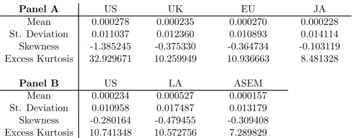
We use Morgan Stanley Capital International (MSCI) international equity index data. We will study six indices: US; Latin America (LA); UK; Developed countries Europe (EU); Japan (JA); Emerging markets Asia (ASEM). Daily data are available from January 1, 1980 (for US, UK, EU and JA), from January 29, 1988 (for LA) and from January 1, 1988 (for ASEM). Summary statistics are in Table 1. Autocorrelograms and cross-correlograms are in Figure 7.

Panel A US UK EU JA Mean 0.000278 0.000235 0.000270 0.000228 St. Deviation 0.011037 0.012360 0.010893 0.014114 Skewness -1.385245 -0.375330 -0.364734 -0.103119 Excess Kurtosis 32.929671 10.259949 10.936663 8.481328 Panel B US LA ASEM Mean 0.000234 0.000527 0.000157 St. Deviation 0.010958 0.017487 0.013179 Skewness -0.280164 -0.479455 -0.309408 Excess Kurtosis 10.741348 10.572756 7.289829

Table 1: Descriptive Statistics: MSCI International Equity Indices. This table reports descriptive statistics for the log-returns of daily MSCI international equity index data. Panel A: Sample period: January 1, 1980 to December 31, 2008. Panel B: Sample period US and Latin America: January 29, 1988 to December 31, 2008; sample period Emerging Markets Asia: January 1, 1988 to December 31, 2008.

We observe from Table 1 that for all the regions under study the Excess Kurtosis is substantially larger than that for a Gaussian distribution. Jumps in equity index returns can cause such Excess Kurtosis. Notice the difference in Excess Kurtosis between the US return series of panel A and the US return series of panel B. This difference is mainly due to the 1987 crisis, the returns of which are included in the longer sample period but not in the shorter sample period.

The plots in Figure 7 exhibit substantial correlations between US returns on day jand returns of other regions of the world on the following day j + 1, except for Latin America where this phenomenon is not pronounced. It becomes apparent from the plots that autocorrelations and cross-correlations die out quickly, so that in five days time (or even fewer) most correlation has disappeared. As discussed in Section 3, the existence of these short-run correlations is where the identification of the self- and cross-excitation parameters comes from.

5.2.

Data Sequencing

The model predicts that the empirical autocorrelation and cross-correlation is decreasing and con-vex, hence that the instantaneous correlation is the largest. Figure 7 plots the empirical autocor-relations and cross-corautocor-relations using the (raw) MSCI data. Due to the fact that different markets operate in different time zones, and the empirical observation that transmission of some markets (US) seems to be stronger than transmission of other markets (non-US) wefind a kink in some of the cross-correlations, for example, US-JA.

To get a qualitative insight in the direction of jump transmissions, we sort daily US returns to

find the most extreme declines (over 3.0% in a single day) in the US stock market in the period January 1, 1980 to December 31, 2008. If the inter-arrival time of these “jumps” was less than

0 1 2 3 4 5 −0.2 0 0.2 0.4 0.6 0.8 1 Correlation j US and UK corr(Δ Xt US ,Δ Xt+j US ) corr(Δ Xt US ,Δ Xt+j UK ) corr(Δ Xt UK ,Δ Xt+j US ) corr(Δ Xt UK ,Δ Xt+j UK ) 0 1 2 3 4 5 −0.2 0 0.2 0.4 0.6 0.8 1 Correlation j US and EU corr(Δ Xt US ,Δ Xt+j US ) corr(Δ Xt US ,Δ Xt+j EU ) corr(Δ Xt EU ,Δ Xt+j US ) corr(Δ Xt EU ,Δ Xt+j EU ) 0 1 2 3 4 5 −0.2 0 0.2 0.4 0.6 0.8 1 Correlation j US and JA corr(Δ Xt US ,Δ Xt+j US ) corr(Δ Xt US ,Δ Xt+j JA ) corr(Δ Xt JA ,Δ Xt+j US ) corr(Δ Xt JA ,Δ Xt+j JA ) 0 1 2 3 4 5 −0.2 0 0.2 0.4 0.6 0.8 1 Correlation j US and LA corr(Δ Xt US ,Δ Xt+j US ) corr(Δ Xt US ,Δ Xt+j LA ) corr(Δ Xt LA ,Δ Xt+j US ) corr(Δ Xt LA ,Δ Xt+j LA ) 0 1 2 3 4 5 −0.2 0 0.2 0.4 0.6 0.8 1 Correlation j US and ASEM corr(Δ Xt US ,Δ Xt+j US ) corr(Δ X t US_{,Δ X} t+j ASEM₎ corr(Δ Xt ASEM ,Δ Xt+j US ) corr(Δ Xt ASEM ,Δ Xt+j ASEM ) 0 1 2 3 4 5 −0.2 0 0.2 0.4 0.6 0.8 1 Correlation j EU and JA corr(Δ Xt EU ,Δ Xt+j EU ) corr(Δ X t EU_{,Δ X} t+j JA₎ corr(Δ Xt JA ,Δ Xt+j EU ) corr(Δ Xt JA ,Δ Xt+j JA )

Figure 7: Autocorrelations and Cross-Correlations (Raw Data). Thisfigure plots autocorrelations and cross-correlations for the log-returns of the daily MSCI international equity data of Table 1. The unit of the indexj is days.

6 weeks, we grouped the returns as being one event, or a related sequence of events. We end up with 63 declines and 23 groups. We read the analysis in the press in the days following each event (statements such as “Tokyo opened lower after Wall Street closed down 3%” vs. “Wall Street opened lower following a rout in European markets”) to confirm the sequencing: where and when the event started, and whether transmission (contagion) took place following one of these events.

Tables 2, 3 and 4 summarize our findings. Generally speaking, we find that it is either (and primarily) a US news announcement that causes the US market to slump, and often such a decline transmits contagiously, or it is a non-US event, typically an adverse shock in emerging markets, and then other regions of the world decline once the US start declining. There are a few exceptions to this general pattern of transmission. In order to cope with the (institutionally introduced) different time zones and hours of operation of the markets around the world some adjustments need to be made to the raw data. We detail below the adjustments made.

5.2.1. US and Japan, and US and Emerging Markets Asia

To get the sequencing right given the time difference, we calculate the instantaneous correlation by leading the Japanese return series by one day. To calculate the lagged cross-correlations we lead the Japanese return series by one day when computingcorr(∆X_tUS,∆X_tJA_+j),j= 1,2, . . ., and we do not