1 INTRODUCTION
Rivers and their associated floodplains form the natural system for the transmission of flood flows. Knowledge of river water levels is essential to flood risk management tasks such as flood risk mapping, strategic planning, scheme design, flood warning and emergency evacuation and channel mainte-nance. In 2001, the Environment Agency of England and Wales commissioned a Targeted Programme of research into reducing uncertainty in conveyance es-timation. The key output was the Conveyance Esti-mation System (CES) software, which provides a practical methodology for estimating flow capacity in rivers, based on the aggregation and extension of previous laboratory derived approaches for applica-tion to natural channels. An essential method re-quirement was the ease of application to rivers of any scale that may be characterised by irregular cross-section shapes, a variety of surface materials, plan form sinuosity and channel braiding.
Previous approaches to calculating flow capacity can broadly be divided into five categories:
1 Hand calculation methods commonly termed Sin-gle and Divided Channel Methods where the channel cross-sectional is treated as a single unit or divided into more than one flow zone
respec-tively. These include, for example, the methods of Manning (1889), Lotter (1933), Yen & Over-ton (1973), Ervine & Baird (1982), Lambert & Myers (1998) and Ackers (1991).
2 Dimensional Analysis approaches where the di-mensionless channel properties such as relative roughness and Froude or Reynolds’ Number are evaluated for scale models and assumed similar for the prototype (e.g. Rameshwaran & Willets, 1999).
3 Additional energy losses due to bends, for exam-ple, the Soil Conservation Service (SCS) and Linearised SCS methods and the work of Chang (1984).
4 Energy ‘loss’ methods which assume that the en-ergy transfers within each flow zone (e.g. main channel or floodplain region) are proportional to the square of the local flow velocity and they are mutually independent and hence the principle of superposition can be applied. Well known meth-ods include those of Ervine & Ellis (1987), James & Wark (1992) and Shiono et al (1999).
5 Reynolds Averaged Navier-Stokes (RANS) ap-proaches, which are based on the depth-integration of the RANS equations for flow in the streamwise direction. Significant research contri-butions include Shiono & Knight (1988), Wark
A practical approach to estimating the flow capacity of rivers –
application and analysis
Ms C. Mc Gahey BSc MSc & Prof P.G. Samuels PhD CEng FIMA MICE MCIWEM
Water Management Department, HR Wallingford Ltd., Howbery Park, Wallingford, Oxon, OX10 8BA, United Kingdom
Prof D.W. Knight BSc MSc PhD CEng MICE MASCE MCIWEM
School of Engineering, University of Birmingham, PO Box 363, Edgbaston, Birmingham, B15 2TT, United Kingdom
ABSTRACT: In 2001, the Environment Agency of England and Wales commissioned a Targeted Programme of Research (Evans et al, 2001) into reducing uncertainty in conveyance estimation, with the intention of bridging the gap between the advances in scientific knowledge over the past three decades and the calculation approaches adopted in United Kingdom industry practice. The key output was the Conveyance Estimation System (CES) software, which incorporates a methodology (Mc Gahey & Samuels, 2003) for estimating con-veyance in a range of channel types and flow conditions, including straight, skewed and meandering plan form shape; simple, two-stage and multi-thread channels; and a variety of vegetation and substrate covers (Defra/EA, 2003; Mc Gahey & Samuels, 2004). In this paper, the CES methodology is applied to fourteen river sites from England, Northern Ireland, New Zealand, Ecuador and Argentina, illustrating reasonable model predictions over a broad application range. Discharge and lateral velocity predictions are compared to observed data, with emphasis on practical application, calibration technique and effects of scale. Considera-tion is given to the relative magnitude of the equaConsidera-tion terms with depth, for example, the role of boundary friction, lateral shear and secondary flows, and how these relate to the observed flow structure and the local site characteristics.
(1993), Abril & Knight (2004), Spooner & Shiono (2003) and Bousmar & Zech (2004).
These previous conveyance approaches have largely focused on experimental channels, which are pris-matic, symmetrical and comprise rectangular or trapezoidal cross-section shapes. Although they pro-vide useful quantifiable parameters for estimating discharge such as width ratios, relative depth, rela-tive roughness and main channel side slopes, they are less useful when applied to rivers with irregular, asymmetrical shapes that may be characterised by distributed roughness or channel braiding. The CES methodology utilizes the ‘as surveyed’ river cross-sections and the observed local roughness features, while incorporating the aforementioned parameter definitions as a guide to understanding and quantify-ing the energy transfer mechanisms, and hence de-riving more universally applicable parameters. This paper demonstrates the broad application range of the CES methodology, through application to four-teen river sites from five countries. An analysis of the relative magnitude of the CES equation terms, i.e. energy transfers due to hydrostatic pressure, boundary friction, lateral shearing and secondary circulations, is undertaken for inbank, main channel overbank and floodplain flow conditions.
2 METHODOLOGY
The methodology is based on the depth-integration of the Reynolds-Averaged Navier-Stokes equations,
[ ]
h y C h q y q f h y h fq ghS uv o ∂ ∂ − + Γ = ⎥ ⎥ ⎦ ⎤ ⎢ ⎢ ⎣ ⎡ ⎟ ⎠ ⎞ ⎜ ⎝ ⎛ ∂ ∂ ⎟ ⎠ ⎞ ⎜ ⎝ ⎛ ∂ ∂ + − ) 1 ( 8 8 2 1 2 2 α α λ ϕ (1)where g = gravitational acceleration (ms-2); q = streamwise unit flow rate (m2s); h = local depth normal to the channel bed (m); So = reach-averaged
longitudinal bed slope; y = lateral distance across the channel (m); ϕ = projection of the boundary shear stress onto the plane due to choice of Cartesian co-ordinate system; and α = function of the reach-averaged sinuosity. Equation 1 has four calibration coefficients: the local friction factor f, the dimen-sionless eddy viscosity λ, the secondary flow pa-rameter Γ and the coefficient of meandering Cuv. The
total flow rate, Q (m3s-1), is hence evaluated from,
∫
≈ bqdy Q0
(2)
where b = the total channel width (m). The fourteen river sites are all located in straight reaches, and thus Equation 1 can be simplified to,
0 8 8 2 1 2 2 = Γ − ⎥ ⎥ ⎦ ⎤ ⎢ ⎢ ⎣ ⎡ ⎟ ⎠ ⎞ ⎜ ⎝ ⎛ ∂ ∂ ⎟ ⎠ ⎞ ⎜ ⎝ ⎛ ∂ ∂ + − h q y q f h y h fq ghSo λ ϕ (3) (1) (2) (3) (4)
where Term 1 is the hydrostatic pressure, Term 2 is the boundary friction, Term 3 is the turbulence due to vertical interfacial shearing and Term 4 represents the secondary circulations due to turbulence in straight channels. The key difference between Equa-tion 3 and the Shiono & Knight (1988) Method (SKM) is the evaluation of f and Γ in natural chan-nels. Here, f is derived from a local unit roughness
nl, which is converted to an equivalent roughness
size, ks, and then the Colebrook-White Law is
incor-porated to evaluate the lateral distribution of f at each flow depth (Mc Gahey & Samuels, 2004). The dimensionless eddy viscosity is derived from (Abril & Knight, 2004),
(
−0.2+1.2 −1.44)
=λmc Dr
λ (4)
where λmc = main channel dimensionless eddy
vis-cosity; and Dr = local relative depth given by h/hmax.
Here, λmc is taken as 0.24 for rivers after Elder
(1959). The secondary flow model Γ, which is based on the work of Abril & Knight (2004), is adapted to incorporate a transitional model Γtrans for asymmetric channels and channels with floodplains at different bed elevations. The main channel inbank, overbank and floodplain formulae are given by (Abril & Knight, 2004), o mci =0.05HρgS Γ ; Γmco =0.15HρgSo; o fp 0.25HρgS Γ =− (5a-c)
where ρ = fluid density (kg m-3). For asymmetric channels or channels with floodplains situated at dif-ferent bed elevations, the secondary flow model in the main channel transitional region is given by (Mc Gahey, in prep.),
(
)
(
) (
l L)
mci L H mci mco trans mc h Z Z Z − − +Γ Γ − Γ = Γ ( ) (6)where ZH and ZL = bed elevation of the higher and
lower floodplains respectively (mAD); and hl =
wa-ter surface level for the given depth of flow (mAD). A further difference is that the CES solution tech-nique is based on the continuity of the unit flow rate
q rather than the depth-averaged velocity as previ-ously used in the SKM approach. This is due to the strong continuity properties of q with variations in depth, for example, across a vertical face or ‘step’ in an engineered channel cross-section (Samuels, 1989; Knight et al, 2004). The approximation to the solu-tion of Equasolu-tion 3 is generated by the Finite Element Method (Defra/EA, 2003b).
3 DESCRIPTION OF DATA SETS
The methodology is applied to fourteen data sets from England, Northern Ireland, New Zealand, Ec-uador and Argentina. These are summarized in Ta-ble 1, including information on bankfull flow rate
Qbf, bankfull depth hbf, main channel width bmc and
the bed slope So. These data sets cover a range of
channel types and scales, notably:
1 Cross-section shape: the river sections are all ir-regular in shape and they include simple (*),
com-pound (**) and asymmetrical (***) shapes (Tab. 1)
as well as a range of aspect ratios (b/h).
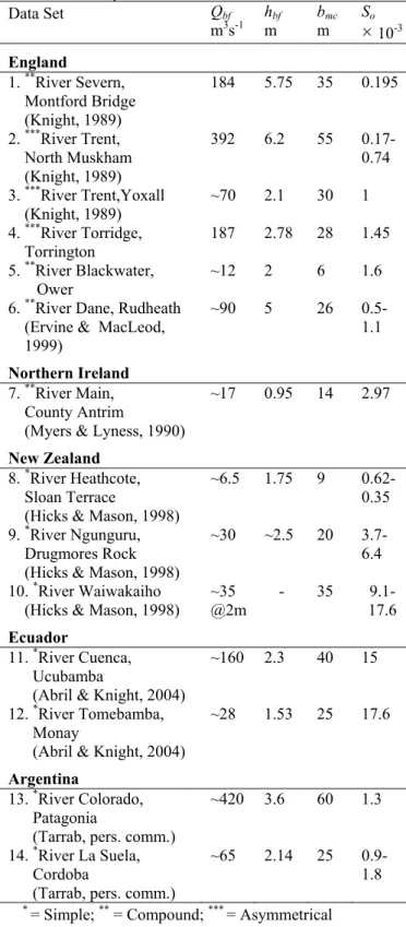
Table 1: Summary of data sets
Data Set Qbf m3s-1 hm bf bm mc So × 10-3 England 1. **River Severn, Montford Bridge (Knight, 1989) 184 5.75 35 0.195 2. ***River Trent, North Muskham (Knight, 1989) 392 6.2 55 0.17-0.74 3. ***River Trent,Yoxall (Knight, 1989) ~70 2.1 30 1 4. ***River Torridge, Torrington 187 2.78 28 1.45 5. **River Blackwater, Ower ~12 2 6 1.6
6. **River Dane, Rudheath (Ervine & MacLeod, 1999) ~90 5 26 0.5-1.1 Northern Ireland 7. **River Main, County Antrim
(Myers & Lyness, 1990)
~17 0.95 14 2.97
New Zealand
8. *River Heathcote, Sloan Terrace
(Hicks & Mason, 1998)
~6.5 1.75 9 0.62-0.35 9. *River Ngunguru,
Drugmores Rock (Hicks & Mason, 1998)
~30 ~2.5 20 3.7-6.4 10. *River Waiwakaiho
(Hicks & Mason, 1998) ~35 @2m - 35 9.1-17.6
Ecuador
11. *River Cuenca, Ucubamba
(Abril & Knight, 2004)
~160 2.3 40 15 12. *River Tomebamba,
Monay
(Abril & Knight, 2004)
~28 1.53 25 17.6
Argentina
13. *River Colorado, Patagonia
(Tarrab, pers. comm.)
~420 3.6 60 1.3 14. *River La Suela,
Cordoba
(Tarrab, pers. comm.)
~65 2.14 25 0.9-1.8 * = Simple; ** = Compound; *** = Asymmetrical
2 Channel cover: the bed, bankside and floodplain ground material includes silt, gravel, cobbles and, small and large boulders well as different vegeta-tion types such as grass, heavy weed growth and fallen trees (Tab. 2).
Table 2: Summary of roughness cover for each channel
River Roughness description
1. Severn Grass-covered floodplains
2. Trent, Mus. Fine gravel & alluvial silts on bed, trees & bushes on floodplain
3. Trent,Yox. Gravel bed, summer in-channel weed growth, grass & bushes on floodplains 4. Torridge Trees on berm
5. Blackwater Vertical sheet piling, fallen trees 6. Dane Thick channel edge growth, less dense
over floodplain
7. Main Coarse gravel bed, quarry stone side slopes, heavy weed growth on berms 8. Heathcote Angular cobbles, gravel, mud & silt on
channel bed, long bankside grass 9. Ngunguru Gravel & cobbles on bed, grazed grass &
scattered brush on banks
10. Waiwakaiho Large boulders (d50 ~2 m), sparse scrub 11. Cuenca Small boulders (d50 ~1 m)
12. Tomebamba Large boulders (d50 ~1.3 m) 13. Colorado Clay bed, rock banks
14. La Suela Alluvial with sparse bankside vegetation
3 Longitudinal bed slope: the data includes steep mountain rivers such as the Cuenca and Tome-bamba as well as more gentle gradients such as the Severn and the Trent.
4 Scale: This includes a range of flow rates and channel sizes, where Qbfranges from 420 m3s-1 in
the Colorado to a mere 7 m3s-1 in the Heathcote and similarly, hbf varies from 1 through to 6 m.
The main channel widths vary from 70 m in the Colorado to 6 m in the Blackwater and the flood-plain widths vary from 500 m in the Dane to 30 m in the Main.
5 Channel braiding: The Torridge and the Black-water are characterised by high banks or ‘levees’ with low adjacent floodplains, which provide an effective channel braiding.
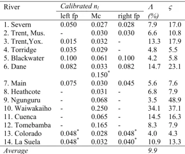
4 VELOCITY AND DISCHARGE PREDICTION Discharge and velocity predictions have been made for the fourteen river sites. The calibration philoso-phy is based on the bed friction only. The input local unit roughness nl, from which the friction factor f is
derived (Mc Gahey & Samuels, 2004), is varied in order to reduce the overall percentage difference Λ
(%) between the predicted QCES and measured flow
rates Qdata i.e.
100 * 1 n Q Q Q i n i data CES data
∑
= − = Λ (7)where n is the number of data points for comparison. The standard deviation ς is given by,
n Q Q Q Q Q Q n i data i CES data i data CES data
∑
= ⎥ ⎥ ⎦ ⎤ ⎢ ⎢ ⎣ ⎡ ⎟⎟ ⎠ ⎞ ⎜⎜ ⎝ ⎛ − − ⎟⎟ ⎠ ⎞ ⎜⎜ ⎝ ⎛ − = 1 2 ς (8)For a given channel cross-section, the unit roughness
nl is provided for a 1m depth of flow, and the
depth-variation of roughness is introduced through the Colebrook-White Law. Once Λ has been minimised i.e. the overall flow predictions are reasonable for the full depth-range, the lateral distribution of nl is
refined in order to best predict the lateral depth-averaged velocity distributions at each depth of flow. This is based on visual inspection of the pre-dicted and measured velocities. The velocity results are shown for three of the sites, selected to illustrate an example of a simple, compound and asymmetri-cal braided channel. Figures 1, 2 and 3 show the depth-averaged velocity predictions for the River Colorado, the River Severn and the River Trent at Yoxall and the calibrated nl values are given in
Ta-ble 3. 0 0.5 1 1.5 2 2.5 3 0 10 20 30 40 50 60 70
Lateral distance across section (m)
De pth-a vera ge d v el oci ty (m. s -1) CES 3.20m CES 2.90m CES 2.49m CES 2.28m CES 2.04m CES 1.90m Data 3.20m Data 2.90m Data 2.49m Data 2.28m Data 2.04m Data 1.90m Scaled bed elevation
Figure 1: Depth-averaged velocity predictions for different flow depths in the River Colorado, Patagonia
0 0.2 0.4 0.6 0.8 1 1.2 1.4 1.6 0 20 40 60 80 100 120 140
Lateral distance across section (m)
Depth-av erag ed vel oci ty ( m .s -1) CES 4.75m CES 6.45m CES 6.92m CES 7.81m Data 4.75m Data 6.45m Data 6.92m Data 7.81m Scaled bed elevation
Figure 2: Depth-averaged velocity predictions for different flow depths in the River Severn at Montford Bridge
The River Colorado tends to under-predict the high velocities at large flow depths and slightly
over-predict the velocities at lower depths. This is most likely a short-coming in the use of the Colebrook-White formulation for establishing the variation of roughness with depth for this wide channel, where bed generated turbulence has a dominant role and the channel banks have less influence. The River Severn data is captured reasonably well, other than the very high velocities in the centre region of the channel. This may indicate that the CES model is over-representing lateral shearing through a large main channel dimensionless eddy viscosity λmc
value of 0.24 in rivers, resulting in an increased re-tarding effect of the slower floodplain flow on the main channel flow. The River Trent data includes measurements for two depths of flow. The predic-tions here are considered reasonable given that the measurements indicate an overall velocity reduction in the main channel for a larger flow depth. For the braided flow depth, the predicted floodplain veloci-ties are supported by the measurements.
In general, the measured velocities are reasonably well-predicted throughout the depth range for the three rivers. 0 0.2 0.4 0.6 0.8 1 1.2 1.4 1.6 1.8 2 0 10 20 30 40 50 60 70 80
Lateral distance across section (m)
D epth-av er ag ed v el oci ty (m.s -1) CES 2.535m CES 2.360m Data 2.535m Data 2.360m Scaled bed elevation
Figure 3: Depth-averaged velocity predictions for two flow depths in the River Trent, Yoxall
Table 3: Summary if unit roughness values, overall percentage flow difference and standard deviation
River Calibrated nl Λ ς left fp Mc right fp (%) 1. Severn 0.050 0.027 0.028 7.9 17.0 2. Trent, Mus. - 0.030 0.030 6.6 10.8 3. Trent,Yox. 0.015 0.032 - 13.3 17.9 4. Torridge 0.035 0.029 - 4.8 5.5 5. Blackwater 0.100 0.061 0.100 4.2 5.8 6. Dane 0.082 0.033 0.150* 0.082 14.7 23.1 7. Main 0.075 0.030 0.045 5.6 7.6 8. Heathcote - 0.031 - 6.8 7.9 9. Ngunguru - 0.068 - 3.5 48.9 10. Waiwakaiho - 0.250 - 34.1 37.1 11. Cuenca - 0.065 - 14.5 16.3 12. Tomebamba - 0.165 - 8.3 7.9 13. Colorado 0.048* 0.028 0.048* 4.0 4.3 14. La Suela 0.048* 0.032 0.040* 10.9 13.3 Average 9.9
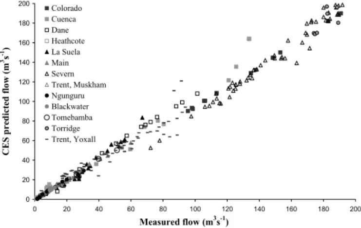
Figure 4 provides a comparison of the predicted flow rates QCES to the measured flow rates Qdata for
all the river sites. A perfect match between the model prediction and the data would yield a gradient of 1.0 i.e. QCES = Qdata. A least squares regression
line gives an R2 value of 0.9889, indicating a ‘good’ fit, and a gradient, i.e. QCES/Qdata, of 0.9822. The
latter is just less than 1.0, suggesting the CES tends to marginally under-predict the flow rate. Figures 4 and 5 demonstrate the range of scales for which the CES predictions are appropriate, from small rivers such as the Heathcote, with flow rates of 7 m3s-1, through to larger rivers such as the Severn, with flow rates in the range 200 to 300 m3s-1, and finally to much large rivers such as the Trent and the Colo-rado, with flow rates upwards of 400 m3s-1. The data shows an increasing degree of scatter with in-creasing flows. This is not surprising since there is more uncertainty associated with river measure-ments taken at high flows, for example, drowned gauge sites, and further to this, the empirically de-rived model coefficients and models such as Equa-tions 4 and 5 for λ and Γ were largely based on labo-ratory measurements. y = 0.9822x R2 = 0.9889 0 100 200 300 400 500 600 0 100 200 300 400 500 600 Measured flow (m3s-1) CE S pr edicted flow (m 3s -1) Colorado Cuenca Dane Heathcote La Suela Main Severn Trent, Muskham Ngunguru Blackwater Tomebamba Torridge Trent, Yoxall
Figure 4: Predicted and measured flow rates for the thirteen river sites 0 20 40 60 80 100 120 140 160 180 200 0 20 40 60 80 100 120 140 160 180 200 Measured flow (m3s-1) CES p re d ict ed fl ow (m 3s -1) Colorado Cuenca Dane Heathcote La Suela Main Severn Trent, Muskham Ngunguru Blackwater Tomebamba Torridge Trent, Yoxall
Figure 5: Predicted and measured flow rates for the thirteen river sites (flow rates < 200m3s-1)
Table 3 provides the overall percentage difference
Λ for each data set, giving an average value for the fourteen data sets of 9.9%. This value is inflated by
the large contributions of the Trent at Yoxall, the Dane, the Waiwakaiho and the Cuenca. For the Trent, this is not surprising considering the afore-mentioned trend in the measured velocity data, where greater flow depths have lower velocities. In addition, there is more uncertainty associated with the floodplain measurements, which are beyond the range of the main channel cableway span, and are therefore based on four overbank gauge points. The Dane is characterised by dense seasonal vegetation, and as the high and low flows are typically measured in different seasons, the vegetation characteristics will be different. This seasonal variation is not in-corporated in the roughness representation. The Waiwakaiho and the Cuenca are steep mountain riv-ers with large bouldriv-ers, and the existing CES meth-odology does not incorporate a model for boulder roughness. Mc Gahey (in prep.) demonstrates the improvement in the CES predictions for mountain rivers through application of the Ramette (1992) ap-proach to evaluate the lateral distribution of f with flow depth. Without these four river sites, the aver-age percentaver-age difference is reduced to 6.2%, sug-gesting a reasonable performance of the CES meth-odology to at least ten river sites.
Table 3 also includes the standard deviation ς for each site. These values tend to be larger than the overall percentage difference Λ, as the expected or mean value is zero i.e. QCES-Qdata, and thus any
variation on this mean has a large value relative to zero. The Ngunguru has the largest ς despite the small value of Λ, indicating a high degree of scatter in the data. The Waiwakaiho has a large ς, which is not unexpected considering Λ is a similar order of magnitude. Likewise, the large ς values for the Dane and the Trent also reflect the large Λ values. For the remaining sites, the standard deviation ς is small and corresponds to the average percentage difference, Λ. This indicates a reasonable model performance in predicting each measured value within each data set, as these measurements are reasonably well-distributed about the CES predicted values. 5 RELATIVE MAGNITUDE OF EQUATION
TERMS
Quantifying the relative magnitude of the four prin-cipal equation terms in Equation 3 is useful in un-derstanding which flow processes have a dominant role, how these mechanisms change with the depth of flow and what channel properties influence these changes. For example, in wide rectangular channels with no vegetation there may be less lateral mixing than in a heavily vegetated irregular-shaped channel. Essential to this is identifying where the relative contributions are the result of a prescribed model within the CES methodology, for example, a change in the role of the secondary flow term between
in-bank and overin-bank flow (Equation 5a-c), compared to external predetermined input parameters such as longitudinal bed slope, channel shape and rough-ness. The average contributions from the different terms are considered for inbank, main channel over-bank and floodplain regions. The river cross-sections and flow depths which are considered are shown in Figures 6 to 16 (placed at the end to aid readability).
Figure 17 provides the relative magnitude of Terms 1 to 4 in Equation 3 for inbank flow condi-tions in seven rivers.
The averages values are 45% hydrostatic pres-sure, 43% boundary shear; 9%, vertical interfacial shear and 2% secondary circulations. The large con-tribution from Term 1 and 2 is not unexpected, as these these constitute the primary balance of forces in the absence of any lateral momentum transfers. Without Terms 3 and 4, Equation 3 would simplify to the well known Darcy-Weisbach equation. The Term 3 contribution is more variable, indicating dif-ferent degrees of lateral shear. In wide shallow channels, the side-walls have less influence on the channel centre and the flow is therefore dominated by bed generated turbulence. The velocity gradient is therefore approximately zero in the channel cen-tre, and the Term 3 contribution is small. In narrow deep channels, the side-walls play a larger role, and there is a greater degree of lateral shearing. Figure 18 provides a plot of the percentage lateral shearing versus aspect ratio where the data trend corroborates this reasoning. 45% 43% 9% 2% 0% 10% 20% 30% 40% 50% 60% 70% 80% 90% 100% Term 1: Hydrostatic pressure Term 2: Boundary friction Term 3: Lateral shear Term 4: Secondary flows Equation term Percent age co nt ributio n River La Suela River Colorado River Severn River Main River Heathcote River Ngunguru River Tomebamba Average
Figure 17: Relative magnitude of equation terms for inbank river flow
The Colorado, the Main, the Waiwakaiho and the Tomebamba all have modest lateral momentum transfers. This is partly due to the large aspect ratios, and partly that the channels have little vegetation and where there is vegetation or boulders there is limited information on the exact location, resulting in the use of average cross-section input unit rough-ness nl values. The Heathcote and Ngunguru have a
greater degree of lateral shearing which may be ex-plained by the large roughness features which en-hance the lateral velocity gradients. The Heathcote has vegetation on the banks and angular cobbles on
the channel bed and the Ngunguru is characterised by gravel and small cobbles.
y = 1.6912x-1.2858 R2 = 0.7712 0% 5% 10% 15% 20% 25% 30% 35% 0 5 10 15 20 25 30 Aspect ratio b/h P ercen ta ge la tera l sh ear (% )
Figure 18: Variation of the percentage lateral shear (Term 3) with aspect ratio
Secondary circulations have a small role in in-bank flow, which is reflected in the low empirically derived ‘0.05’ value in Equation 5a, and hence through the small contribution of Term 4.
Some of the rivers differ from the more general trend, for example, the River Severn has a low hy-drostatic pressure term and a high degree of lateral shear relative to the other sites. The former may re-sult from incorporating a representative reach-averaged longitudinal slope based on measured wa-ter levels for at high flow depths, whereas in reality the surface water slope at Montford Bridge varies substantially with depth (Knight, 1989a). The latter may be attributed to the dense channel vegetation.
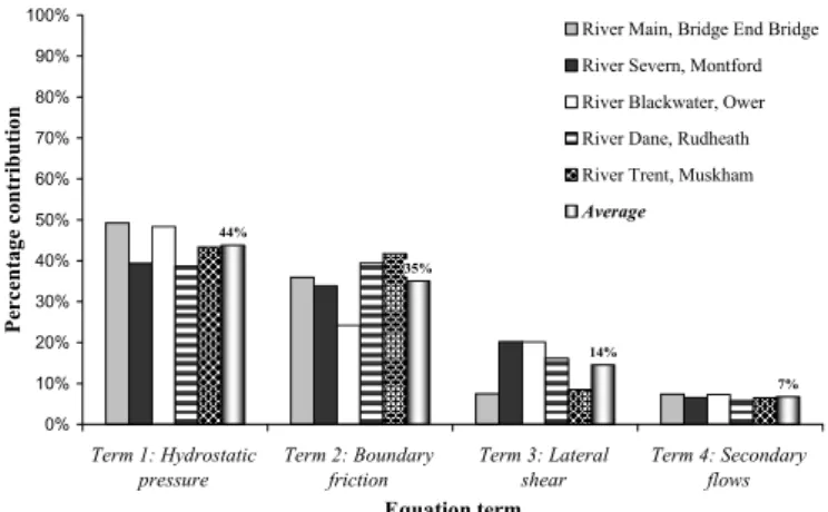
Figure 19 provides the relative magnitude of Terms 1 to 4 in Equation 3 for main channel over-bank flow conditions in five rivers. The averages values are 44% hydrostatic pressure, 35% boundary shear; 14%, vertical interfacial shear and 7% secon-dary circulations. 44% 35% 14% 7% 0% 10% 20% 30% 40% 50% 60% 70% 80% 90% 100% Term 1: Hydrostatic pressure Term 2: Boundary friction Term 3: Lateral shear Term 4: Secondary flows Equation term Pe rcentag e contribution
River Main, Bridge End Bridge River Severn, Montford River Blackwater, Ower River Dane, Rudheath River Trent, Muskham
Average
Figure 19: Relative magnitude of equation terms for main channel flow in two-stage rivers
The Severn and the Dane have small hydrostatic pressure contributions, which may be related to the high degree of lateral shearing present in the deep narrow main channel regions. As with the inbank case, the Main has substantially less lateral shearing, than for example, the Severn, as there is less
vegeta-tion present and the conveyance is therefore largely geometry driven.
The Blackwater has a noticeably small boundary friction contribution. This is most likely related to the cross-section geometry, in that the irregular ge-ometry results in local steep velocity gradients and hence large lateral momentum transfers. This is re-flected in the high lateral shear contribution, which off-sets the boundary friction term in balancing the hydrostatic pressure.
The secondary flow contribution for all sites is more than double that of the inbank flow sites, re-flecting the larger ‘0.15’ value in Equation 5b.
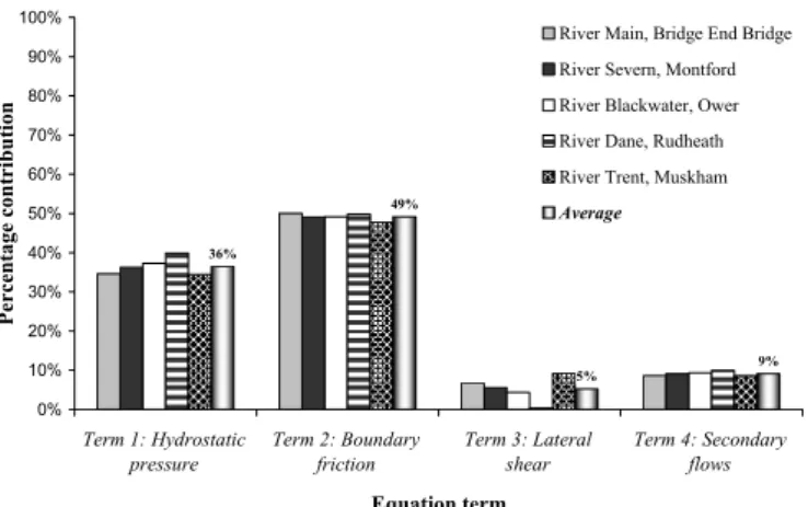
Figure 20 provides the relative magnitude of Terms 1 to 4 in Equation 3 for the floodplain flow conditions. The averages values are 36% hydrostatic pressure, 49% boundary shear; 5%, vertical interfa-cial shear and 9% secondary circulations.
The average hydrostatic pressure term is substan-tially smaller for floodplain flow, which may be at-tributed to the lower floodplain flow depths and the high boundary friction due to the presence of dense floodplain vegetation. The most variable contribu-tion is the vertical interfacial shear. This is approxi-mately zero for the Dane, which may be explained by the low floodplain depths. Conversely, the Trent has the highest lateral shear, which results from the steep velocity gradient at the floodplain main chan-nel interface coupled with the relatively short flood-plain width i.e. the inundated floodflood-plain extent is not sufficiently wide to achieve a constant lateral veloc-ity gradient.
The average secondary flow contribution is large, reflecting the large value of the prescribed CES model coefficient in Equation 5c.
36% 49% 5% 9% 0% 10% 20% 30% 40% 50% 60% 70% 80% 90% 100% Term 1: Hydrostatic pressure Term 2: Boundary friction Term 3: Lateral shear Term 4: Secondary flows Equation term Perce nta ge con tribution
River Main, Bridge End Bridge River Severn, Montford River Blackwater, Ower River Dane, Rudheath River Trent, Muskham
Average
Figure 20: Relative magnitude of equation terms for floodplain flow in two-stage rivers
6 CONCLUSIONS
A practical approach to estimating the flow capacity of rivers has been demonstrated for fourteen rivers sites from five different countries, where the unit roughness nl was the only calibration parameter. The
depth-averaged velocity predictions compared
rea-sonably well to the measured data for a simple, compound and asymmetrical river example over a range of flow depths. The predicted QCES and
meas-ured Qdata flows for fourteen river sites showed a
least squares regression fit of 0.9889, which is close to an ideal fit of 1.0. The ratio of QCES to Qdata was
0.9882, suggesting that the CES is more likely to slightly under-predict than over-predict the meas-ured flow values. The average percentage difference
Λ between the measured and predicted flows for all sites was 9.9%, demonstrating the effectiveness of the model over a range of scales and channel types. This value may be reduced to 6.2% if the mountain-ous rivers with large boulders are excluded. The CES methodology is therefore a useful approach for application in river engineering practice, as it incor-porates models and parameters that can readily be applied to natural channels, over a range of scales, with irregular geometries, roughness features and channel braiding.
An analysis of the relative magnitude of the four equation terms in Equation 3 was undertaken for in-bank, overbank and floodplain flow. As expected, the hydrostatic pressure and the boundary shear terms were large and they constituted the primary force balance. The boundary friction term was ~10% higher in the floodplain region due to low flow depths and greater vegetation roughness. The lateral shearing term was the most variable. For inbank flows, the variations were shown to be closely re-lated to the aspect ratio. For overbank flow, this was dependent on the floodplain flow depths, where for low or very high floodplain depths, the floodplain flow has less retarding influence on the main chan-nel flow. For main chanchan-nel overbank flow, the de-gree of lateral shearing is linked to vegetation growth. The secondary flow contributions are gener-ally small relative to the other equation terms, with a larger contribution in compound channels.
This analysis is useful in practice as it enables practitioners to focus their attention on particular river features. For example, river surveys should ideally include detailed descriptions of the exact cross-section location and nature of vegetation fea-tures. It further draws attention to the importance of the main channel dimensionless eddy viscosity λmc
value as well as the rule applied in Equation 4, which may not always be appropriate in describing the lateral shearing in two-stage rivers.
7 RECOMMENDATIONS
The CES methodology has been demonstrated for fourteen river sites, all located in straight river reaches. For further testing, it is recommended that a targeted data acquisition programme is imple-mented, where the data collection focuses on straight and meandering two-stage natural channels, and
measurements include discharge, water level, depth-averaged velocities and, where possible, turbulence measurements.
The methodology incorporates the Colebrook-White Law to evaluate the lateral distribution of the friction factor for each depth of flow. For mountain streams with boulders, an alternative formulation, such as the method of Ramette (1992) is recom-mended.
The importance of the lateral shearing term in two-stage channels is highlighted. Thus, further in-vestigation of the applicability of Equation 4 for the lateral distribution of the dimensionless eddy viscos-ity λ in two-stage rivers is advocated.
8 ACKNOWLDEGEMENTS
This paper draws upon the Targeted Programme of research commissioned by the Environment Agency (EA) of England and Wales as project W5A-057 un-der the joint the Department for Environment, Food and Rural Affairs (Defra) / EA Flood and Coastal Defence R&D Programme. We wish to thank Dr Mervyn Bramley, the Agency Project Manager for his encouragement and support. The views ex-pressed in this paper are, however, personal and the publication does not imply endorsement by either the EA or Defra. The Authors wish to acknowledge Professor Boris Abril and Miss Leticia Tarrab for their contributions to data.
REFERENCES
Abril, J.B. & Knight, D.W. 2004. Stage-discharge prediction for rives in flood applying a depth-averaged model. Jnl. of Hydraulic Research, IAHR. 42(6): 616-629.
Ackers, P. 1991. Hydraulic design of straight compound chan-nels. SR Report 281. HR Wallingford, UK, 1&2: 1-130 & 1-140.
Bousmar, D. & Zech, Y. 2004. Velocity distribution in non-prismatic compound channels. Proc. ICE, Water Manage-ment, 157: 99-108.
Chang, H.H. 1984. Regular meander path model, Jnl. of Hy-draulic Eng. ASCE, 110(10): 1398-1411.
Defra/EA, 2003. Reducing uncertainty in river flood convey-ance. Roughness Review. Project W5A- 057, HR Walling-ford, UK.
Defra/EA, 2003b. Reducing uncertainty in river flood convey-ance. Interim Report 2 - Review of Methods for Estimating Conveyance. Project W5A- 057, HR Wallingford, UK. Elder, J.W. 1959. The dispersion of marked fluid in a turbulent
shear flow. Jnl. Fluid Mechanics, 5(4): 544-560.
Ervine, D.A. & Baird, J.I. 1982. Rating curves for rivers with overbank flows. Proc. ICE Part 2: Research and Develop-ment, 73: 465-472.
Ervine, D.A. & Ellis, J. 1987. Experimental and computational aspects of overbank floodplain flow. Trans. of the Royal Society of Edinburgh: Earth Sciences. 78: 315-475.
Ervine, D.A. & MacLeod, A.B. 1999. Modelling a River Channel with Distant Floodbanks, Proc. Institution Civil Engineers Water, Maritime and Energy. 136: 21-33.
Evans, E.P., Pender, G., Samuels, P.G. & Escarameia, M. 2001. Reducing Uncertainty in River Flood Conveyance: Scoping Study, R&D Technical Report to DEFRA / Envi-ronment Agency. Project W5A- 057. HR Wallingford Ltd. UK.
Hicks, D.M. & Mason, P.D. 1998. Roughness Characteristics of New Zealand Rivers. NIWA. Christchurch. 1-329. James, C.S. & Wark, J.B., 1992, Conveyance estimation for
meandering channels SR 329, pp 1-91, HR Wallingford, UK.
Knight, D.W. 1989. River Channels and Floodplains, Final Re-port for Severn Trent Water Authority. April, 1-100. Knight, D.W., Omran, M. & Abril, J.B., 2004, Boundary
con-ditions between panels in depth-averaged flow models re-visited, Proc. of the 2nd Intl. Conf. on Fluvial Hydraulics: River Flow 2004, 1: 371-380, Naples, 24-26 June.
Lambert, M.F. & Myers, W.R.C. 1998. Estimating the dis-charge capacity in straight compound channels. Proc. ICE Jnl. for Water, Maritime and Energy, Paper 11530, 130: 84-94.
Lotter, G.K. 1933. Considerations on hydraulic design of chan-nels with different roughness of walls. Trans. All-Union Scientific Research Institute of Hydraulic Eng., Leningrad, 9: 238-241.
Manning, R. 1889. On the flow of water in open channels and pipes. Trans. ICE of Ireland. 20: 161-207.
McGahey, C. in preparation. A practical approach to estimating the flow capacity of rivers. PhD thesis, Open University, Milton Keynes, UK.
McGahey, C. & Samuels, P.G. 2003. Methodology for convey-ance estimation in two-stage straight, skewed and meander-ing channels, Proc. XXX IAHR Congress, Thessaloniki, C1: 33-40.
Mc Gahey, C. & Samuels, P.G. 2004. River roughness – the in-tegration of diverse knowledge. Proc. 2nd International
Conference on Fluvial Hydraulics. River Flow 2004.
Naples. 24-26 June. 1: 405-414.
Myers, W.R.C. & Lynness, J.F. 1990. Flow resistance in rivers with floodplains. Final Report on research grant GR/D/45437. University of Ulster. UK.
Rameshwaran, R. & Willets, B.B. 1999. Conveyance predic-tion for meandering two-stage channel flows. Proc. ICE
Jnl. for Water, Maritime and Energy, Paper 11765, 136:
153-166.
Ramette, M. 1992. Hydraulique et morphologie des. rivières: quelques principes d’etude et applications. Compagnie Nat-inale du Rhone, Formatione Continue, France.
Shiono, K. & Knight, D.W. 1988. Two-dimensional analytical solution for a compound channel. Proc. 3rd Intl. Sympo-sium on Refined Flow Modelling and Turbulence Meas-urements. Universal Academy Press. 591-599.
Shiono, K., Muto, Y., Knight, D.W. & Hyde. A.F.L., 1999, Energy losses due to secondary flow and turbulence in me-andering channels with overbank flow, Jnl. of Hydraulic Research, IAHR, 37(5): 641-664.
Spooner, J. & Shiono, K. 2003. Modelling of meandering chan-nels for overbank flow. Proc. ICE Jnl. for Water, Maritime and Energy, 156: 225-233.
Yen, C.L. & Overton, D.E. 1973. Shape effects on resistance in floodplain channels. Jnl. of the Hydraulics Division, ASCE, 99(1): 219-238.
CROSS-SECTION FIGURES 6 TO 16 0 1 2 3 4 5 6 7 8 9 0 20 40 60 80 100 120 140
Lateral distance across section (m)
B ed ele va tion ( m )
Figure 6: River Severn, Montford
0 2 4 6 8 10 12 0 50 100 150 200 250 300 350 400
Lateral distance across section (m)
B ed e lev at ion (m )
Figure 7: River Trent, North Muskham
0 0.5 1 1.5 2 2.5 3 0 10 20 30 40 50 60
Lateral distance across section (m)
B ed ele va tion ( m )
Figure 8: River Blackwater, Ower
10 11 12 13 14 15 16 17 18 19 20 0 100 200 300 400 500 600
Lateral distance across section (m)
B ed ele va tion ( m )
Figure 9: River Dane, Rudheath
0 0.5 1 1.5 2 2.5 3 0 5 10 15 20 25 30 35 40
Lateral distance across section (m)
B ed ele va tion (m )
Figure 10: River Main, County Antrim
0 0.5 1 1.5 2 2.5 0 2 4 6 8 10
Lateral distance across section (m)
B ed ele va tion ( m )
Figure 11: River Heathcote, Sloan Terrace
0 0.5 1 1.5 2 2.5 3 3.5 4 4.5 0 2 4 6 8 10 12 14 16 18 20
Lateral distance across section (m)
B ed ele va tion ( m )
Figure 12: River Ngunguru, Drugmores Rock
0 1 2 3 4 5 6 0 5 10 15 20 25 30 35 40
Lateral distance across section (m)
B ed ele va tion ( m )
Figure 13: River Waiwakaiho, SH3 0 0.2 0.4 0.6 0.8 1 1.2 1.4 1.6 1.8 0 5 10 15 20 25 30 35 40
Lateral distance across section (m)
Bed e lev at io n ( m )
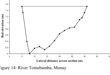
Figure 14: River Tomebamba, Monay
0 0.5 1 1.5 2 2.5 3 3.5 0 5 10 15 20 25 30 35 40
Lateral distance across section (m)
B ed ele va tion ( m )
Figure 15: River La Suela, Cordoba
0 1 2 3 4 5 6 0 10 20 30 40 50 60 70 80
Lateral distance across section (m)
B ed ele va tion ( m )