Confidence Estimation in Image-Based Localization

(1)

CONFIDENCE ESTIMATION IN

IMAGE-BASED LOCALIZATION

Faculty of Information Technology and Communication Sciences Master’s Thesis November 2019

(2)

ABSTRACT

Luca Ferranti: Confidence Estimation in Image-Based Localization Master’s Thesis

Tampere University

Electrical Engineering, MSc November 2019

Image-based localization aims at estimating the camera position and orientation, briefly re-ferred as camera pose, from a given image. Estimating the camera pose is needed in several applications, such as augmented reality, odometry and self-driving cars. A main challenge is to develop an algorithm for large varying environments, such as buildings or whole cities. During the past decade several algorithms have tackled this challenge and, despite the promising results, the task is far from being solved. Several applications, however, need a reliable pose estimate; in odometry applications, for example, the camera pose is used to correct the drift error accumulated by inertial sensor measurements. Based on this, it is important to be able to assess the confi-dence of the estimated pose and manage to discriminate between correct and incorrect poses within a prefixed error threshold. A common approach is to use the number of inliers produced in the RANSAC loop to evaluate how good an estimate is. Particularly, this is used to choose the best pose from a given image from a set of candidates. This metric, however, is not very robust, especially for indoor scenes, presenting several repetitive patterns, such as long textureless walls or similar objects. Despite some other metrics have been proposed, they aim at improving the ac-curacy of the algorithm, by grading candidate poses referred to the same query image; they thus recognize the best pose among a given set but cannot be used to grade the overall confidence of the final pose. In this thesis, we formalize confidence estimation as a binary classification prob-lem and investigate how to quantify the confidence of an estimated camera pose. Opposed to the previous work, this new research question takes place after the whole visual localization pipeline and is able to compare also poses from different query images. In addition to the number of in-liers, other factors such as the spatial distributions of inin-liers, are considered. A neural network is then used to generate a novel robust metric, able to evaluate the confidence for different query images. The proposed method is benchmarked using InLoc, a challenging dataset for indoor pose estimation. It is also shown the proposed confidence metric is independent of the dataset used for training and can be applied to different datasets and pipelines.

Keywords: Confidence Estimation, Visual Localization, Computer Vision, InLoc, Neural Networks The originality of this thesis has been checked using the Turnitin OriginalityCheck service.

(3)

TIIVISTELMÄ

Luca Ferranti: Luottamuksen Estimointi Kuvapohjaisessa Paikannuksessa Diplomityö

Tampereen yliopisto Sähkötekniikka, DI Marraskuu 2019

Kuvapohjainen paikannus pyrkii estimoimaan kameran sijainnin ja asennon annetusta kuvas-ta. Tätä voidaan soveltaa esimerkiksi lisättyyn todellisuuteen, odometriaan tai automatisoituihin autoihin. Estimointi osoittautuu haastavaksi muuttuvissa ympäristöissä, kuten kaupungeissa tai suurissa sisätiloissa ja viime vuosien nopeasta kehittymisestä huolimatta kuvapohjainen paikan-nus on edelleen avoin tehtävä. Sovellukset vaativat kuitenkin luotettavaa estimointia, sillä esi-merkiksi odometriassa estimoituja kameran sijaintia ja asentoa käytetään inertiasensoreiden mit-tauksista kasaantuneen virheen korjaamiseen. Tämän johdosta kyky arvioida estimoinnin luo-tettavuutta on olennainen tehtävä. Tähän mennessä mittarina on monesti käytetty RANSAC-algoritmissa esiintyvää malliin sopivien pisteiden (inliers) määrää. Tämä mittari ei kuitenkaan sovellu esimerkiksi sisätilapaikannukseen, jossa kuvioiden toistuvuuden takia epätarkalla esti-moinnilla voi olla myös suuri määrä malliin sopivia pisteitä. Tässä opinnäytetyössä luottamuksen estimointia formuloidaan binäärisenä luokittelutehtävänä ja kehitetään neuroverkkopohjaista me-netelmää, jolla kvantisoida estimoidun kameran sijainnin ja asennon luotettavuutta. Menetelmä opetetaan ja testataan InLoc-datasetin avulla, joka on haastava sisätilapaikannukseen tarkoitettu datasetti. Työssä osoitetaan myös, että kehitetty menetelmä on opetuksessa käytetystä datase-tistä riippumaton ja sitä voidaan soveltaa myös muihin datasetteihin.

Avainsanat: Luottamuksen Estimointi, Kuvapohjainen Paikannus, Konenäkö, InLoc, Neuroverkot Tämän julkaisun alkuperäisyys on tarkastettu Turnitin OriginalityCheck -ohjelmalla.

(4)

PREFACE

This thesis was written during autumn 2019 in the computer vision research group in Aalto University. The supervisors were Jani Boutellier (Tampere) and Juho Kannala (Aalto). The examiners were Jani Boutellier and Esa Rahtu (Tampere).

First, I would like to thank my supervisors Jani and Juho for their guidance and espe-cially for the precious feedback I have been constantly given. Without you, this thesis would not exist and even if it did, it would be much worse. I am also grateful for all the amazing colleagues I have been working with, both in Tampere and in Espoo. Having a comfortable work environment was definitely a necessary condition for the success of this thesis. I also want to thank my friends from Tampere University for the time spent studying together and, most importantly, for the time spent not studying. We really had a lot of fun during these years! Moreover, many thanks also to all my friends and relatives for the support and understanding during my whole life. Last, but definitely not least, I wish to thank my fiancée Lotta Tapanainen for her immeasurable love and support.

Tampere, 19th November 2019

(5)

LIST OF FIGURES

2.1 Geometric interpretation of homogeneous coordinates. . . 5

2.2 Illustration of the pinhole camera model. . . 6

2.3 Parallelism is not preserved during 3D-2D mapping. . . 7

2.4 Camera general pose. . . 10

3.1 Visualization of the pose estimation problem [19]. . . 13

3.2 Geometrical formulation of the P3P. . . 15

3.3 Pseudocode of RANSAC algorithm. . . 17

3.4 Visualization of SIFT descriptor. . . 20

3.5 Active search pipeline. . . 23

3.6 Typical pipeline of image retrieval based localization. . . 24

3.7 Full-frame coordinate regression [23]. . . 26

3.8 Example pictures from the dataset. . . 28

3.9 Pipeline of InLoc algorithm. . . 29

3.10 Accuracy as a function of translation threshold, angular threshold being10◦. 30 4.1 Example of an inaccurate estimate with a high number of inliers. . . 34

4.2 Number of inliers distributions. . . 35

4.3 Failure due to a repetitive pattern [35]. . . 36

4.4 Coverage scores distributions. . . 37

4.5 Incorrect estimate with many inliers covering a small area. . . 38

4.6 Cameras similarities distributions. . . 39

4.7 Proposed network architecture. . . 40

5.1 PR-curve of InLoc using the number of inliers as discriminator. . . 43

6.1 Precision-recall curves obtained with our method. . . 44

6.2 Performances of coverage score as discriminator. . . 47

6.3 Verification score performances as confidence estimator. . . 49

6.4 Inclusion of InLoc verification score to our method. . . 49

6.5 Verification score distributions. . . 50

6.6 Comparison of accuracies with our method and with InLoc. . . 51

6.7 Qualitative comparison of best candidate poses with InLoc (left, inliers highlighted in blue) and our method (right, inliers highlighted in red), both including PV. First row: InLoc error: 32 m, 3.9◦. Our error: 0.09 m, 3.7◦. Second row:InLoc error: 5.3 m,14.3◦. Our error:0.24 m,2.9◦.Third row: InLoc error: 0.56 m,2.1◦. Our error:4.4 m,2◦. . . 52

(8)

LIST OF TABLES

3.1 Dataset properties per image group. . . 27

3.2 Dataset properties per floor. . . 28

3.3 Computation times of different steps for a single query image. . . 31

6.1 Performances of the proposed method at different error threshold. . . 45

6.2 Ablation study of the proposed model. The full network contains inliers, cameras differences and cov. scores. . . 46

6.3 Coverage score improving InLoc accuracies. . . 47

6.4 Accuracies with different candidates sorting methods. . . 51

6.5 Performances of our InLoc trained algorithm in Cambridge Landmarks dataset. 53 6.6 Improved accuracies on Aachen when adding our method to the pipeline of [22]. . . 54

(9)

LIST OF SYMBOLS AND ABBREVIATIONS

α, β, γ angles

ANN Artificial neural network AUC Area Under Curve

C Camera position in real world coordinates CNN Convolutional neural network

∼ Equivalence relation

η Inliers coverage score

f, fx, fy Focal length

Inls Inliers

K Camera intrinsic parameters matrix

λ Scalar parameter for scale invariance

L Loss function NN Nearest neighbor ∥ · ∥ Euclidean norm P Projection matrix Pn Projective space PnP Perspective-n-point p Precision

px, py Principal point offset coordinates

q Quaternion

R Rotation matrix

RANSAC Random sample consensus

r Recall

Rn Euclidean space

SIFT Scale-invariant feature transform

t Translation vector

tr(·) Trace of a matrix

w Added coordinate when mapping fromRntoPn

(10)

x Image point

x, y Coordinates in 2D vector space

(11)

1 INTRODUCTION

We, human beings, are able to extract information about our environment simply relying on what we see. For centuries people have been able to orient themselves using just a map and their eyes. This leads to the question Could machines do the same? Given a camera and some information about the environment, can a computer orient itself? In the field of computer vision, i.e. the automatic analysis of images, this question is known as image-based localization (or visual localization, or camera pose estimation) [25]. In a more formal way, image-based localization aims at computing the camera position and orientation, together shortly referred as camera pose, from a given image when the environment is known. Mathematically, knowing the environment means to know the coordinates of the 3D points in it and computing the pose of a camera means to find a mapping between the 3D points of the environment and the 2D points in the image. In pose estimation problems, it is also assumed that the internal parameters of the camera are known.

An accurate camera pose estimation is necessary in several applications. In robotics, autonomous vehicles need to keep track of the path they have travelled. This motion tracking problem, known as odometry [51], is generally tackled with inertial sensor mea-surements. Nevertheless, inertial sensors accumulate measurement errors, which makes the estimated position too inaccurate after a few minutes of motion. To overcome this problem, a reliable external signal, measuring the position of the device, must be used to correct the accumulated error. In outdoor environment, this task is accomplished by GNSS/GPS [9]. As GNSS signals are not detectable inside buildings, new solutions are needed for indoor odometry. Together with RF based (e.g. WiFi) positioning [21, 55], visual localization offers appealing possibilities for inertial odometry, as some state-of-the-art algorithms can already be run in real-time on mobile devices [26, 27]. Augmented Reality (AR) also requires information about the camera pose [31]. As objects are per-ceived differently in shape and size depending on the point of view of the observer, adding realistic-looking objects requires knowledge about the camera position and orientation.

In a typical pose estimation pipeline, the environment is known to the machine through a large database of images, for which the original 3D coordinates of the pixels, and hence also the camera pose, are known. When a query image in fed into the algorithm, it will first retrieve the most similar images from the database, form correspondences between points in the query and database images and then use the correspondences to compute the camera pose. As multiple database images are retrieved for a single query image,

(12)

multiple candidate poses will be produced. Computing the camera pose is generally an ill-posed problem, meaning after the computation only some correspondences will agree with the proposed camera. These correspondences are called inliers. The pose with the highest number of inliers will be chosen as the best candidate and outputted as final result.

Despite the improvements achieved in the past years [35, 36, 48], image-based localiza-tion is still far from being solved. High accuracies are achieved for simple stalocaliza-tionary cases [17, 23], where the environments are relatively small and do not undergo big changes. However, realistic applications, such as self-driving cars, require pose estimation in large varying environments, such as whole cities or buildings. Clearly, the same square will appear completely different in winter or in summer, or even during different hours of the same day. Consequently, retrieving similar database images and forming correspon-dences will be challenging. On the other side, large environments have generally certain redundancy. For example, the same windows may appear on opposite sides of a building, which may introduce some wrong correspondences between query and database image. Indeed, sometimes estimating the pose may not be even possible. Let us consider the case of indoor visual localization and suppose our query image shows only a light switch on a white wall, without any additional details. Clearly, this picture cannot be used to reliably estimate the pose. A building can have hundreds of identical light switches and knowing which one of them is in the picture is impossible without further details. Still, our algorithm will compute a pose and it may also return a high number of inliers if an identical light switch is found from a database image.

The previous paragraph opens the questionHow reliable my estimate is? Research so far has focused on finding the best pose from a set of candidates and several metrics, also more robust than the number of inliers, have been developed. Still, these metrics do not answer our question, as the best pose among a set of candidates can still be wrong. For this reason, confidence estimation, investigated in this thesis, is a relevant research question. Failure is just something to cope with and for an algorithm being able to critically analyze the results and recognize unreliable estimates is just as important as giving an accurate one. Our philosophy to tackle the confidence estimation problem can be divided into two steps: first, in the analysis step, we try to identify what factors particularly affect the success of pose estimation, starting from empirical observations from state-of-the-art datasets. Next, in the synthesis step, we seek for an algorithm that can combine the knowledge obtained from observations, producing a measure of the confidence of the pose.

This thesis is structured as follows: in Chapter 2 we review the mathematical foundations of geometric computer vision, i.e. how to model image formation and how to parametrize the camera, particularly focusing on how to represent its pose. In Chapter 3 the visual localization task is presented, as well as an analysis of the algorithms used to solve it. A typical visual localization pipeline is dissected, analyzing the implementations of its core elements, which are common to most state-of-the-art approaches. We also present

(13)

the main modern pipelines used to solve the problem. The pipelines are presented in a comparative way, focusing on the strengths and weaknesses of each of them. In Chapter 3 the Inloc dataset and algorithm are also introduced, as they are later used to benchmark the proposed confidence estimation algorithm. Chapter 4 is dedicated to confidence modelling. First, singular factors affecting the success of the estimate are presented, using images from InLoc to show why they are relevant from a confidence estimation point of view. Next, it is described how these factors can be brought together to obtain a final confidence estimation measure. In Chapter 5 the executed numerical experiments are described, together with the used evaluation metrics. In Chapter 6 the results are then presented and discussed. Finally, in Chapter 7 the results and the main points of the thesis are summarized and an overview of possible future work is given.

(14)

2 GEOMETRIC COMPUTER VISION

In this chapter we review the theoretical background behind geometric computer vision, needed to understand the key issues of this thesis. First, we introduce the projective space, which is the mathematical structure used to describe the geometrical properties of images. The description will be short and focused on the results needed later. The purpose is to make the reader understandwhythe abstract concepts of projective spaces capture the geometric essence of computer vision. Next, we will introduce the pinhole camera model, the simplest mathematical model describing image formation. Finally, we will extend this model to describe real world cameras, obtaining a complete framework to mathematically describe image formation, needed to understand later the problem of visual localization.

2.1 Projective space

The space we live in can be modelled as a vector space, calledEuclidean spaceR3. This

means the position of each point can be expressed by a vector of three real numbers

[X, Y, Z]T, called Cartesian coordinates. A picture taken with a camera is a 2D

repre-sentation of 3D objects. In other words, taking a picture means toproject points from a 3D space into a 2D space. This 3D-2D double nature of images is not described well by Euclidean spaces. We introduce thus a fundamental tool used in computer vision, the

projective space[8].

Definition 2.1. Given an Euclidean spaceRn, the projective spacePnisPn⊆Rn+1\{0}

equipped with the equivalence relation ∼ so that x ∼ y ⇔ ∃λ ̸= 0 : x = λy1. The coordinates of a point in the projective space are calledhomogeneous coordinates. Let us now dissect this definition to understand its meaning. The first part tells us the dimension of the space, so a point in the 2D-projective space P2 will have three

coor-dinates and a point in the 3D-projective space P3 will have four coordinates. Also, the

point with all zeros coordinates is not allowed. The second part tells us that points in the projective space areunique up to scale, meaning in_P2 _{the coordinates} _[1_,₂_,_3]T _and [2,4,6]T _{represent the same point. Cartesian coordinates can be converted to}

homoge-1_{This actually means that the projective space is a} _{quotient space}_{, and we could compactly write}

(15)

neous coordinates and vice versa with equations (2.1) and (2.2), respectively. [x1, x2, . . . , xn]T ↦→[x1, x2, . . . , xn,1]T, (2.1) [x1, x2, . . . , xn, w]T ↦→ [x₁ w, x2 w,· · · , xn w ]T . (2.2)

We will now highlight some important geometrical properties of projective spaces, which will help understand later why projective geometry is a suitable model for computer vision. We will describe these properties usingP2as an example, but the same concepts can be

extended toP3as well.

First, we analyze the points in the form [x, y,0]T, with x ̸= 0 or y ̸= 0. According to Equation (2.2), this point will map to [_x

0,

y

0

]T

= [∞,∞]T_{. For this reason, points of the}

form[x, y,0]are calledpoints at infinity. It can be proved that these points lie on the same

line, which is calledline at infinity. With this new concept the following fundamental result can be proved:

• Parallel lines in R2 are incident in P2 and their intersection point is on the line at

infinity. x z y x1 λ1x1 λ2x1 x2 λ1x2 λ2x2

Figure 2.1. Geometric interpretation of homogeneous coordinates.

We give now a geometrical interpretation to the equivalence relation in the definition of projective space. Letx∈_P2_{, all points in the form}_λ_x_{, λ}_̸_{= 0}_{will correspond to the same}

point. If we interpret the homogeneous coordinates inP2 as Cartesian coordinates inR3,

the set of pointsλxforms a line going through the origin, as depicted in Figure 2.1. This means that a point inP2 can be interpreted as a line through the origin inR3, noting that

by definition of projective space the origin ofR3 is excluded. This can be summarized as

the following fundamental result:

• There is a one-to-one correspondence between points in P2 and lines passing

(16)

2.2 Pinhole camera model

Mathematically speaking, taking a picture means mapping points in the 3D space to points in a 2D plane, thus it can be described as an operatorP :R3 →R2. The coordinate

system in the 3D space is called real world coordinate system and its points real world points. Similarly, the 2D plane where the image is formed is called image plane, its coordinate systemimage coordinate systemand its pointsimage points.

Z Y X x y x X C p f

Figure 2.2. Illustration of the pinhole camera model.

The simplest model describing this operator is thepinhole camera model [15], illustrated in Figure 2.2. To be able to analyze this and further models, some terms need to be defined:

• Camera centerC: position of the camera in the real world coordinate system,

• Principal pointp: Center of the image plane,

• Focal lengthf: distance between principal point and camera center,

• Ray: line connecting a real-world point and the camera center,

• Principal axis: ray connecting camera center and principal point.

In this model, a point in the real world coordinate system Xis mapped to a the pointx, obtained as the intersection between the image plane and the ray passing throughX. If the image plane were infinite, all points in the 3D space could be mapped to the image plane. However, cameras have a limited aperture, meaning the image plane will be finite.

The pinhole camera model models a camera under several strict assumptions. These assumptions can be divided into two groups: those regarding how the coordinate systems are defined and those regarding camera internal properties. The first set of assumptions requires that the origin of the real world coordinate system is at the camera center and the origin of the image coordinate system is at the principal point. Furthermore, theXandY

(17)

axes of the real world coordinate system are aligned with thexandy axes of the image coordinate system. The second set of assumptions regards the technical properties of the camera, namely that pixels are squares, the image plane is rectangular and straight lines are not distorted when projected. If these assumptions hold, it can be derived that

P : ⎡ ⎢ ⎢ ⎢ ⎣ X Y Z ⎤ ⎥ ⎥ ⎥ ⎦ ↦→ ⎡ ⎣ f X Z f Y Z ⎤ ⎦. (2.3)

Equation (2.3) shows thatP is a nonlinear operator. It can be noticed that this mapping introduces some loss of information. First, information about the 3D point depth (i.e. Z -coordinate) is lost. It can also be shown that ratios of lengths, angles between lines and parallelism is not preserved, as shown in Figure 2.3. Several tasks in computer vision consist in retrieving knowledge about 3D structures, such as depth, distances, shapes, from 2D images. Due to the loss of information, these tasks are usuallyill-posed, meaning that the existence and uniqueness of the solution cannot be guaranteed.

Figure 2.3. Parallelism is not preserved during 3D-2D mapping.

From Figures 2.2 and 2.3 two interesting properties can be noticed. First, each point in the image plane lies on only one ray, meaning there is a one-to-one correspondence be-tween 2D points and 3D lines passing through the camera center. Second, parallel lines in the Euclidean space intersect each others when projected into the image plane.

(18)

Fur-thermore, the intersection points are all on the same line. Both of these properties were already encountered in the previous section, when the projective space was introduced. Based on this, the projective space seems to capture those geometrical properties that could not be formalized in Euclidean space. Rewriting the operator as a mapping be-tween projective spaces,P :P3 →P2 Equation (2.3) becomes

P : ⎡ ⎢ ⎢ ⎢ ⎢ ⎢ ⎢ ⎣ X Y Z 1 ⎤ ⎥ ⎥ ⎥ ⎥ ⎥ ⎥ ⎦ ↦→ ⎡ ⎢ ⎢ ⎢ ⎣ f X f Y Z ⎤ ⎥ ⎥ ⎥ ⎦ . (2.4)

Equation (2.4) is indeed correct because points in homogeneous coordinates are unique up to scale, hence [f X, f Y, Z]T _∼[f X

Z , f Y

Z ,1

]T

, as in (2.3). Using homogeneous coor-dinates leads also to another important result. Let X= [X, Y, Z,1]T and x = [x, y, w]T

corresponding 3D and 2D points in homogeneous coordinates, now (2.4) becomes

x= ⎡ ⎢ ⎢ ⎢ ⎣ f 0 0 0 0 f 0 0 0 0 1 0 ⎤ ⎥ ⎥ ⎥ ⎦    =P X=PX, (2.5)

where the matrixP is called theprojection matrix. Equation (2.5) shows that when using homogeneous coordinates the operator P is actually linear and can be defined as a matrix. This is a fundamental result, which allows us to exploit linear algebra tools in numerical applications. Problems involving linear operators are also numerically simpler to solve. Due to their advantages and wide use in computer vision, in this thesis we will assume all points are in homogeneous coordinates, unless explicitly stated differently. The most important exception being the camera centerC, which will always be assumed to be in euclidean coordinates.

2.3 Real camera model

So far we have analyzed the idealized pinhole camera model. As seen, it requires several strict assumptions, which hardly ever hold in real-life applications. In this section we will investigate how our model changes when these assumptions do not hold, until reaching a more generalreal camera model, which replaces the pinhole camera model in real life applications.

(19)

2.3.1 Intrinsic parameters

Intrinsic parameters describe camera internal properties. A first assumption says that pixels are square. Pixels shape needs to be taken into account because pixels are the unit of measure in image points coordinates. Practically this means that the focal length in (2.5), whose unit is naturally meters, needs to be converted to pixels. If the pixel is not square, the focal length will scale differently in horizontal and vertical directions, leading to two different focal lengths fx = αxf and fy =αyf, whereαx and αy are respectively

the reciprocals of pixel width and height in meters.

Another assumption was the origin of the image coordinate system being on the principal point. As pixel indexing generally starts either from the left-most upper corner, with the

y-axis pointing down or from the left-most lower corner, with they-axis pointing up, this assumption does not hold. This means the principal point will not be at the origin of the image coordinate system, but it will have an offset (px, py), i.e. the projected point

has to be translated by the offset to have the right coordinates. With these observations Equation (2.5) becomes x= ⎡ ⎢ ⎢ ⎢ ⎣ fx 0 px 0 0 fy py 0 0 0 1 0 ⎤ ⎥ ⎥ ⎥ ⎦ X. (2.6)

The last assumptions were the image plane being rectangular, meaning the image coordi-nate system is orthogonal, and straight lines being preserved when projected. If these do not hold, the model can be further generalized taking into account cameraskew [13] and

lens distortion [11]. For the case studies considered in this thesis, however, we can as-sume those assumptions to hold and hence we will not discuss them any further. Finally, the process of determining camera intrinsic parameters is known as camera calibration

[16]. A camera is said to becalibrated if its intrinsic parameters are known.

2.3.2 Extrinsic parameters

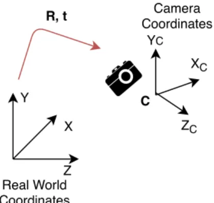
Extrinsic parameters describe camera position and orientation, i.e. the camera pose, with respect to the real world coordinate system. In the pinhole model, it was assumed that real world and image coordinate systems were aligned and that the origin of the real world coordinate system was in the camera center. As the real world reference system a fixed inertial frame is generally used, breaking this assumption. To model this, let us define thecamera coordinate systemas the reference frame obeying the pinhole model, i.e. with origin onCand axes aligned with image axes, as shown in Figure 2.4. Given a real world pointX, a change of coordinates has to be performed before applying equation (2.6), i.e. we must first convertXtoXC whose coordinates are expressed in the camera

(20)

X Y X_C Z ZC YC Real World Coordinates C Camera Coordinates R, t

Figure 2.4.Camera general pose.

The camera coordinate system frame can be obtained from the original frame with a rotation to align the axes and a translation to align the origins. Thus, to obtain the point

XC in camera coordinates, we need to apply the euclidean transformation

⎡ ⎢ ⎢ ⎢ ⎣ XC YC ZC ⎤ ⎥ ⎥ ⎥ ⎦ =R ⎡ ⎢ ⎢ ⎢ ⎣ X Y Z ⎤ ⎥ ⎥ ⎥ ⎦ +t, (2.7)

whereRis a rotation matrix andtis a translation vector. Equation (2.7) can be written in homogeneous coordinates as XC = ⎡ ⎣ R t 03×1 1 ⎤ ⎦X. (2.8)

The rotation matrixRaligns the axes of the coordinate frames. Intuitively, axes alignment can be done aligning one axis at a time, i.e. by a combination of three rotations around axesX Y andZof the real world coordinate systems with anglesα,βandγrespectively. The rotation matrices around the axes of a given angle are defined as

Rx(α) = [ 1 0 0 0 cosα −sinα 0 sinα cosα ] , Ry(β) = [ cosβ 0 sinβ 0 1 0 −sinβ 0 cosβ ] , Rz(γ) = [ cosγ −sinγ 0 sinγ cosγ 0 0 0 1 ] , (2.9)

where the notationRe(θ)indicates a rotation around axiseof angleθ. The total rotation matrix can thus be written as

R=Rx(α)Ry(β)Rz(γ), (2.10)

meaning we will first rotate around thez-axis, then around the y-axis and finally around thex-axis. Equation (2.10) reveals that the rotation matrix, despite having nine elements, has only three degrees of freedom, represented by the angles α, β and γ, which are calledEuler angles[15].

(21)

that the rotation matrixR describes also a single rotation around the axis eof angle θ, i.e. the frames can be aligned with a single rotation. The existence of the rotation axise

implies

Re=e, (2.11)

because the rotation axis does not change during the rotation. Equation (2.11) gives a way to compute the rotation axis, as it says eis the eigenvector of R corresponding to the eigenvalueλ= 1. The existence ofealso implies we can construct a frame in which

R is in one of the forms in equation (2.9), which leads to equation (2.12) to compute the rotation angle θ= arccos ( tr(R)−1 2 ) . (2.12)

Vice versa, given the rotation axiseand angleθthe rotation matrix can be computed with equation (2.13), which is called Rodrigues rotation formula

R=I+ sinθ ⎡ ⎢ ⎢ ⎢ ⎣ 0 −ez ey ez 0 −ex −ey ex 0 ⎤ ⎥ ⎥ ⎥ ⎦ + (1−cosθ) ⎡ ⎢ ⎢ ⎢ ⎣ 0 −ez ey ez 0 −ex −ey ex 0 ⎤ ⎥ ⎥ ⎥ ⎦ 2 . (2.13)

Based on the analysis so far, a 3D rotation can be described by a 3x3-matrix, by three euler angles or by an axis and an angle. This last result implies that rotations can be represented as a quadruple. Given the axis e and angle θ we define the associated quadruple q= [ cos(θ₂) exsin (_θ 2 ) eysin (_θ 2 ) ezsin (_θ 2 )]T . (2.14)

The quadruple in equation (2.14) is called quaternion [28]. The analysis of algebraic properties of quaternions is beyond the scope of this thesis. For our purposes, it is enough to define the norm of a quaternion as in equation (2.15)

∥q∥=√a2₊_b2₊_c2₊_d2_, _(2.15)

wherea, b, c, dare the components of the quaternionq.

The axes being aligned, we want next to bring the origin of the rotated frame to the cam-era center. Let Cthe camera center euclidean coordinates in the real world coordinate system. After the rotation the new coordinates will beRC. To bring this point to the origin we need to apply a translation with vector

t=−RC. (2.16)

The vector in equation (2.16) is in euclidean coordinates and it has three degrees of freedom. It can be concluded that the camera pose has six degrees of freedom, three arising from the rotation matrix and three arising from the translation vector. This result is in accordance with classical mechanics, which says a rigid body in the 3D euclidean

(22)

space has six degrees of freedom in total. Finally, equations (2.6) and (2.8) can be combined obtaining x= ⎡ ⎢ ⎢ ⎢ ⎣ fx 0 px 0 0 fy py 0 0 0 1 0 ⎤ ⎥ ⎥ ⎥ ⎦ ⎡ ⎣ R t 03×1 1 ⎤ ⎦X= ⎡ ⎢ ⎢ ⎢ ⎣ fx 0 px 0 fy py 0 0 1 ⎤ ⎥ ⎥ ⎥ ⎦    :=K [ R t ] X =K [ R t ] X =K [ R −RC ] X. (2.17)

Equation (2.17) gives the real camera model. The matrixK models camera intrinsic pa-rameters and hence it is calledintrinsic matrixand matrix[R t

]

models camera extrinsic parameters, i.e. position and orientation and it is calledcamera pose.

(23)

3 IMAGE-BASED LOCALIZATION

So far we have developed a mathematical model to describe how a camera transforms 3D coordinates into 2D coordinates. This framework helps us understand the problem ofimage-based localizationalso known ascamera pose estimationorvisual localization. Formally, the visual localization problem can be expressed as followsGiven a query im-age, what was the pose of the camera?, i.e. what was its position and orientation, when the image was taken? A visualization of this question is given in Figure 3.1: a query image is taken with a smartphone and the algorithm infers the position and orientation of the camera and is able to locate it in a map of the environment (indicated with a red pyramid).

Figure 3.1. Visualization of the pose estimation problem [19].

Visual localization is a calibrated problem, meaning that the intrinsic parameters of the cameras used are known. Furthermore, visual localization algorithms require a "map" of the environment where the query image was taken. This map can be either a database of images for which the original 3D coordinates of most of the pixels are known or a 3D dense model of the environment. Further information about how these can be constructed can be found e.g. in [53] and [37]. In a traditional visual localization pipeline two main steps can be identified: formation of correspondences between 2D and 3D coordinates and pose estimation from points correspondences. In this chapter we first analyze these two phases, focusing on the methodologies used. Next, we present the structure of some typical state of the art approaches. Finally, we analyze more in details InLoc, a pipeline

(24)

for indoor visual localization, which will serve as case study in this thesis.

3.1 Pose Estimation from points correspondences

Let the correspondence(x,X)and intrinsic matrix K. Equation (2.17) can be simplified introducing the normalized coordinates corresponding to x, defined as u = K−1x =

[u, v, w]T. Thus, the correspondence equation becomes

λu=[R t

]

X, (3.1)

where the parameter λ ̸= 0 was introduced because homogeneous coordinates are unique up to scale, meaning a pose satisfying the mapping X ↦→ λu is still a solution of the original problem. First, we investigate what is the smallest number of correspon-dences needed for the problem to have a finite number of solutions. Equation (3.1) can be written as λ ⎡ ⎣ u v ⎤ ⎦= ⎡ ⎢ ⎢ ⎢ ⎣ r11 r12 r13 tx r21 r22 r23 ty r31 r32 r33 tz ⎤ ⎥ ⎥ ⎥ ⎦ ⎡ ⎢ ⎢ ⎢ ⎢ ⎢ ⎢ ⎣ X Y Z 1 ⎤ ⎥ ⎥ ⎥ ⎥ ⎥ ⎥ ⎦ ⇔ ⎧ ⎪ ⎪ ⎪ ⎨ ⎪ ⎪ ⎪ ⎩ λu=r11X+r12Y +r13Z+tx λv =r21X+r22Y +r23Z+ty λw =r31X+r32Y +r33Z+tz , (3.2)

we can now divide the first and second equation by the third one in (3.2) obtaining

⎧ ⎨ ⎩ u w = r11X+r12Y+r13Z+tx r31X+r32Y+r33Z+tz v w = r21X+r22Y+r23Z+ty r31X+r32Y+r33Z+tz . (3.3)

Equation (3.3) shows that for each point correspondence we get two independent nonlin-ear equations. It was shown in the previous chapter that the camera pose has six degrees of freedom, hence at least three point correspondences are needed to solve the system in Equation (3.3).

3.1.1 Perspective-n-Point

The family of algorithms used to estimate the camera pose fromnpoint correspondences are referred as Perspective-n-Point solvers (PnP), where the parameter nindicates the number of correspondences used. Based on the previous discussion,n≥3is needed for the system to be determined. Next, we investigate the uniqueness of the solution. This is

(25)

addressed exploiting Gao’s formulation of the P3P problem [54], which is widely used in several software implementations.

C X′₃ X′1 X′₂ u3 u2 u1 z y x a b c ϕ θ ψ

Figure 3.2. Geometrical formulation of the P3P.

The setup for Gao’s solver is shown in Figure 3.2. Let the correspondences (u1,X′1),

(u2,X′2) and (u3,X′3) between image points in normalized homogeneous coordinates

and real world points in Euclidean coordinates. By the law of cosines we obtain

⎧ ⎪ ⎪ ⎪ ⎨ ⎪ ⎪ ⎪ ⎩ a2 =x2+y2−2xycosθ b2 =y2+z2−2yzcosϕ c2 =x2+z2−2xzcosψ , (3.4)

wherex=∥X1−C∥,y=∥X2−C∥andz=∥X1−C∥. The cosines can be computed from

the 2D points coordinates, e.g. cosθ = u1·u2

∥u1∥·∥u2∥. The system (3.4) is the formulation of

P3P algorithm used in Gao’s solver, several algebraic techniques have been proposed to efficiently solve the system [56]. Oncex,yandzhave been solved, the camera position

Ccan be found by trilateration, that is computing the intersection of the spheres centered onX′₁,X′₂ and X′₃ and with radiix,yandz respectively. From Figure 3.2, it is clear that this intersection isC. Next, equations (3.1) and (2.16) can be combined obtaining

λiui =R(X′i−Ci), (3.5)

from which follows

|λi|∥ui∥=∥X′i−C∥, (3.6)

The value of λcan now be found from equation (3.6). We can safely drop the absolute value and assumeλis positive, as the sign can be corrected later. Finally, the rotation matrix can be computed from (3.5) – first we find the rotation axis e= ui×(X′i−C)

∥ui×(X′i−C)∥ and

the rotation angleθas the angle betweenui and(X′i−C). The rotation axis and angle

(26)

formula can be applied to obtainR. It should be noticed that for the obtained matrix holds

det(R) =±1. The rotation matrix, however, requiresdet(R) = 1, hence ifdet(R) =−1,

Randλshould be corrected changing their sign.

The system (3.4) has degree eight, meaning that it admits up to eight distinct solutions. The amount of solutions can be reduced introducing physical constraints. It can be proved that four of these solutions place the camera center on the wrong side of the image plane. After discarding physical unacceptable candidates the P3P leads to four possible camera poses. Further constraints can be generated requiring invariant properties of projective geometry to be preserved, leading finally to a unique solution. Alternatively, the ambi-guity in the P3P algorithm can be removed introducing further point correspondences. In the P4P algorithm, for example, the solving system is derived from four points corre-spondences. This leads to a unique solution if the four 3D points lie on the same plane, otherwise it leads to five feasible solutions. The P6P algorithm leads to a unique so-lution, moreover P6P algorithm allows to solve the elements of the rotation matrix and translation vector directly from (3.2), making the problem linear.

In general, introducing further correspondences reduces the degree of the solving equa-tion, reducing ambiguity. Also, a higher number of correspondences produces faster solvers. Despite maybe sounding controversial at the beginning, introducing more points correspondences produces more geometrical knowledge about the system, which can be exploited to reduce the final degree of the solving equation; for example, the P3P solver led to a system of degree eight, whereas in the P6P solver the solving system is linear. Furthermore, as more points correspondences reduce ambiguity, less postprocessing is needed to identify the correct solution. However, it should be beared in mind that our discussion so far assumed the points coordinates and the correspondences to be exact. In practical applications this does not hold. First, due to noise points coordinates them-selves contain some uncertainty, hence the coordinates cannot be assumed to be exact. Second and more important, as we will discuss in the next section, forming points corre-spondences is the most challenging part in visual localization pipelines and a significant amount of wrong matches is introduced. Feeding bad matches to a PnP solver leads to absurd results. As discussed in the next subsection, solvers are generally iterated sev-eral times to deal with wrong matches and using a smaller number of correspondences increases the probability to pick only good matches at least once. The more correspon-dences are used, the smaller this probability and consequently, despite being the inner solver faster, the number of iterations needed increases, resulting in an overall slower algorithm.

3.1.2 RANSAC algorithm

The main problem with PnP solvers is their sensibility to input data. A small error in points correspondences can lead to a completely different camera pose. State-of-the-art approaches still introduce a significant amount of wrong correspondences, which are

(27)

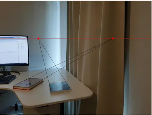
calledoutliers. Consequently, pose estimation algorithms need to be robust to outliers. A popular choice to estimate parameters with outliers is the Random Sample Consen-sus (RANSAC) algorithm [10]. Given N correspondences(u,X), we randomly pickkof them and estimate the camera posePˆ. Next, we compute the number of inliers, i.e the number of correspondences for which d(u,PˆX) ≤ t, whered(·,·) andtare chosen dis-tance measure and threshold. The process is iterated and at the end the model with the highest number of inliers is outputted. The parameters to be adjusted are the distance function, the threshold and the maximum number of iterations. In image-based local-ization applications a popular choice for the distance measure is the angular distance

d(u,PˆX) =∠(u,PˆX)with a threshold of a few degrees, e.g. t= 1◦. The maximum num-ber of iterations is chosen so that at least once thek randomly picked correspondences contain only inliers with probabilityp(e.g. p= 0.99). Letethe outliers ratio, the number of maximum iterations satisfying this property can be computed asNmax = _log(1log(1₋₍₁−₋p_e)₎k₎. In

practical applications the outlier ratio is not known, hence it is estimated and updated dur-ing the RANSAC algorithm. The pseudocode of the RANSAC algorithm with P3P solver is shown in Figure 3.3.

Figure 3.3. Pseudocode of RANSAC algorithm.

During the years several modifications of the basic RANSAC algorithm have been pro-posed to improve its performances [33]. A popular variation used in visual localization is the locally optimized-RANSAC (LO-RANSAC) [6], which introduces a smaller inner RANSAC loop. Once a pose hypothesis and its inliers are computed (line 8 in Figure 3.3), a new RANSAC is started, sampling now only from the current set of inliers. Clearly, this reduces the probability of picking an outlier, hence in the inner RANSAC it is not strictly necessary to use the minimum amount of samples. The new hypothesis and the number of inliers are computed and the process is then iterated, keeping as best model the one with the highest number of inliers. Differently from the outer loop, the inner loop is generally iterated a fixed amount of times. At the end, the best model hypothesis, together with the new set of inliers are outputted from the inner loop, substituting the

(28)

original ones computed in the outer loop.

3.2 Forming points correspondences

So far we have discussed how to estimate the camera pose given 2D-3D correspon-dences, in this section we will analyze the problem of how to form these correspondences. Suppose we have a picture and a dense 3D model of the environment where the picture was taken, a point in the image will correspond to a point in the 3D model if they corre-spond to the same point in the real world. Ideally, each point in the image correcorre-sponds to exactly one point in the 3D model. In practical applications, however, this is not possi-ble, nor useful. First of all, a query image taken with a common smartphone can easily have millions of pixels, which would make matching every point extremely time consum-ing. Second, some zones of the image carry almost no information and are not useful for finding correspondences, for examples pixels in a flat homogeneous zone. Based on this, we first want to identifygood pointsfrom the image and then find their corresponding 3D coordinates. Once the set of good points has been identified, a method to compare points has to be defined. Intuitively, corresponding points will represent the same object, such as the same corner of the same monitor, or the same eye of the same person. Coordi-nates however only tell where the points are but have no information about their meaning. For this reason we need to create a semantical representation of the points, in which in-formation about the content of the image is embedded. Practically, this means that a functionf :Pn→ Rk has to be designed. This function, calleddescriptor, associates to

a given point ak-ary vector, calledfeature vector which models the semantic meaning of the point. As points are adimensional, descriptors generally consider the neighbourhood of a point. Finally, finding the corresponding point means to find themost similar vector, i.e. a distance measure to compare feature vectors is needed. Based on this discussion, the correspondences forming problem can be formulated as a Nearest Neighbour (NN) problem [7], as in Equation (3.7).

X= argmin Xi

d(f(x), g(Xi)), (3.7)

wherexandX are corresponding 2D and 3D points,f and g are descriptors andd(·,·)

is a distance function. As feature vectors are vectors in the Euclidean space, a popular distance function is the Euclidean distance.

The described approach, despite being correct and giving state-of-the-art accuracies, is not very efficient, as 3D models are generally dense and hence have billions of points. Despite efficient search methods have been developed, solving the NN problem is still too time consuming, especially if the algorithm is required to run real time on a mobile device. For this reason an alternative approach is to perform 2D-2D matching. The dense model is replaced by a database of images for which the 3D coordinates of the pixels are known. For a given query image, the most similar database images are retrieved and

(29)

points correspondences are formed between pixels in the query and database images. The NN problem in (3.7) is hence modified as in (3.8)

xdb= argmin xi

d(f(xq), f(xdb)), (3.8)

wherexq and xdb are now points in the query and database image, respectively. Since

we are now comparing two 2D images, the same descriptorf is generally used for both. As this approach has become far more popular and can be also applied to a several range to tasks, beyond visual localization, we will describe here some popular descriptors and distance functions for 2D-2D matching. A brief overview of descriptors for 2D-3D matching will given in 3.3.1 where an example of direct matching pipeline is analyzed. Here we assume that relevant database images have already been retrieved, how the retrieval process works is discussed in 3.3.2.

3.2.1 Traditional descriptors

In order to solve the NN problem of Equation (3.8) first the interest points need to be found and then the descriptorf as well as the distance measuredneed to be defined. Ideally,

f(x1) = f(x2) if and only ifx1 and x2 correspond to each others. The semantic content

of the image is taken into account by observing the neighbourhood of the pixels, which allows to capture local properties of points. Particularly, relevant semantic information can be detected by computing the gradients of the pixel. Suppose to have a flat black zone in the image, all pixels in that area will be indistinguishable from each others and hence they will not be good feature points. Mathematically, these pixels have zero directional derivatives in each direction. On the other hand, pixels with accentuated changes in their neighbourhoods will contain more information and hence work nicely as feature points. Interest points can thus be found by looking for pixels with strong intensity gradients. Based on this analysis, the following problem arises: the interest points detector depends on the scale of the image, as zooming closer would attenuate the gradients. To overcome this problem, the search is done at different resolutions, i.e. consecutively downsampling the image and performing the search at each resolution level [4]. A common algorithm to detect interest points is the Harris corner detector and its implementation details can be found in [47].

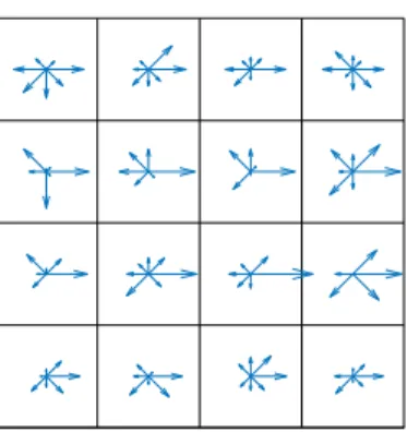
Once the interest points have been detected, a meaningful descriptor has to be applied to it. A popular choice is the Scale-Invariant Feature Transform (SIFT) descriptor [29]. Simi-larly to features detection, SIFT descriptor relies on the assumption that gradients can be used to model semantic meaning. The SIFT descriptor can be computed as follows: for a given feature point, a 16x16 neighbourhood around it is formed. This neighbourhood is then divided into sixteen 4x4 smaller cells. In each cell, the gradient for each pixel is computed. We then consider the eight main directions, spaced by 45◦, i.e. similarly to the directions of a compass. Each computed gradient is then aligned to its closest main

(30)

direction and aligned gradients are summed, obtaining eight gradients for each cell, as depicted in Figure 3.4. The magnitudes of these form an 8-ary array calledhistogram of oriented gradients for each cell. Each so obtained array is circularly shifted so that the strongest gradient is the first element of the array. As the original neighbourhood was divided into sixteen cells and eight gradients were computed in each cell, the final result is a 128-ary array, which is the final descriptor associated with the considered interest point. The SIFT descriptor is translation invariant, as gradients are computed and scale invariant, as interest points were detected at different resolutions. Furthermore, circularly shifting the arrays in each cell introduces also rotation invariance.

(a)Original gradients. (b)Clustered gradients.

Figure 3.4. Visualization of SIFT descriptor.

Once SIFT descriptors have been computed for both query and database images, a distance measure has to be defined to match points from query and database images. As SIFT descriptor is a vector in the _R128 _{space, vectors can be compared by simply}

using the euclidean distance as distance measure. It can be proved, however, that better performances are achieved using the Hellinger distance defined as

H(v,u) =∥√v−√u∥2, (3.9)

where√vindicates the element-wise square root of the array. The popularity of Hellinger distance led to a modified version of SIFT, known as rootSIFT, which is obtained as fol-lows: given a SIF descriptor v, it is first L1-normalized, i.e. each element is divided by the sum of the absolute values of the elements, then the square root of each element is taken and finally the so obtained array is normalized by its euclidean norm. The so obtained rootSIFT descriptors can then be compared by the normal Euclidean distance, i.e. rootSIFT descriptors with Euclidean distance is equivalent to using SIFT descriptors with Hellinger distance in (3.9) [3]. We have now a recipe to solve the NN problem in (3.8), once all descriptors have been computed they can be stored in appropriate data structures for efficient search algorithms, such as kd trees [43].

The presence of redundancy and noise in both database and query images can lead to wrong matches when applying the NN algorithm. Particularly, if several similar descriptors

(31)

are found, the nearest is not necessarily the correct one. To improve the robustness of the algorithm, given a feature vector in the query image v, the two closest neighbours

u1 andu2 are retrieved from the database image, withd(v,u1) < d(v,u2), i.e. u1 is the

closest match. Next, the correspondence(v,u1)is accepted only if

d(v,u1)

d(v,u2)

< γ, (3.10)

where γ is a predetermined threshold, generally around 0.7 or 0.8. Equation (3.10) is known asLowe’s ratio test [30] at it makes sure that only the most confident inliers are kept.

Despite Lowe’s ratio test improves the robustness, a relatively high number of wrong matches is generally still returned. A further improvement is to use a verification step, given a set of points {xq1,xq2, . . . ,xqN} from the query image and the corresponding

points{xdb1,xdb2, . . . ,xdbN} from the database image, all in homogeneous coordinates,

we try to fit a transformation H : xqi ↦→ xdbi, λxdbi = Hxqi. The transformation H

between projective planes is calledhomography and it can be computed with algorithms similar to pose estimation within a RANSAC loop [15]. Once the best homography is computed, the inliers outputted from RANSAC form the final set of correspondences.

3.2.2 Deep learning based descriptors

The approaches described so far for points matching were human-reasoning based, meaning first the algorithm designer fixes what properties a good interest point and a good descriptor should have and then derives a mathematical formulation to compute them. Feature vectors have thus a physical interpretation, understandable to humans. For example, the SIFT descriptor extracts the gradients in a neighbourhood of an interest point, because gradients characterize the shape of the neighbourhood and hence cap-ture its semantical meaning. Deep learning methods, on the other hand, let the computer "learn" by itself what a good descriptor should look like and how to compute it. This is implemented exploiting neural networks, which can be regarded as black boxes, taking images as input and outputting interest points and the corresponding feature vectors. Opposed to traditional methods, a human-understandable explanation of why those are considered good points and why descriptors are computed that way cannot generally be given. The interest for neural networks has exponentially risen in the past decade, reaching state-of-the-art solutions for several artificial intelligence problems, also beyond computer vision.

In the context of computer vision, and image processing in general, Convolutional Neural Networks (CNN) are particularly attractive [42], as the mathematical definition of 2D con-volution allows to capture local and global properties of images. The constitutive unit of a convolutional neural network is generally composed by three layers: convolutional, ac-tivation and pooling. The convolutional layer consists of a set ofK 2-dimensional filters,

(32)

each applied to the input image. If the input size isH ×W ×3 (hence a RGB image), the output will have size H ×W ×K, such multidimensional structures are generally called tensors. The activation step applies a nonlinear function to each element of the previous tensor. Popular activation functions are, for example, arctanhor the Rectified Linear Unit (ReLU)ReLU(x) = max(0, x), the activation layer does not change the size of the tensor. The pooling layer performs downsampling in the first two dimensions, for example keeping every other element, outputting a tensor of sizeH/2×W/2×K. A CNN is obtained stacking several times the described units. The tensors outputted after each unit are calledfeature maps and in visual localization pipelines they are used to perform points matching. Before it can be used, the network needs to learnto produce relevant feature maps. Practically, this means that the coefficients of the filters in the convolutional layers need to be determined. To train a neural network, the last feature map is first flat-tened into a N-ary array which is, possibly after some intermediate layers, mapped to a scalar through a functionL, calledloss function. The parameters of the networks are determined minimizing the loss function. Designing and training neural networks is a field of its own, for our purpose it is enough to understand the basic structure of a CNN and how it relates to visual localization. There is plenty of literature about neural networks and further information about their structure and training algorithms can be found e.g. in [14].

In the context of features matching, the feature map of sizeH×W×Kcan be interpreted as a set ofH·K interest points, each associated with a K-ary feature vector. Matching can now be done with a NN algorithm, i.e. for each feature vector in the query feature map the most similar is found from the database image feature map. Points matching with feature maps is generally referred asdense matching. As discussed, several feature maps are produced by the intermediate layers of a CNN. As they are consequently down-sampled, they become sparser and sparser as they propagate through the network. This rises the questionWhat feature map should be used? Using a too sparse feature map will weaken the accuracy of interest points coordinates and using a very fine feature map will, on the other side, result into a significantly time consuming process, unacceptable for e.g., real-time applications. To solve this,coarse-to-fine matching is used, where two feature maps of sizes H1 ×W1×K1 and H2 ×W2×K2 are used, withK1 > K2 and

W1 > W2, i.e. the first one is the fine feature map and the second one is coarse feature

map. Point matching is first done with the coarse feature maps. Once the correspon-dences are found, the corresponding points in the fine maps are taken and the matching accuracy is improved performing NN search in their neighbourhoods.

As a final remark, deep learning based descriptors generally produce more robust cor-respondences compared to traditional descriptors. Nevertheless, the final result may still and probably will contain several wrong matches, due to the challenging and ill-posed nature of the problem. From an accuracy point of view, forming correspondences is gen-erally the bottle-neck of visual localization pipelines.

(33)

3.3 Typical image-based localization pipelines

As shown in the previous section, designing a pose estimation pipeline leaves the pro-grammer some freedom, such as choosing the matching strategy or the kind of the de-scriptors. To concretize the previous discussion, we present here some popular state of the art pipelines, that have been recently developed to address long-term visual localiza-tion.

3.3.1 Direct matching

In direct matching approaches, points correspondences are directly formed between the 2D query image and the 3D model. Several approaches have been proposed to compute descriptors of 3D point clouds. For example, it is possible to generalize the SIFT de-scriptor to the 3D case considering a volumetric neighbourhood of a given interest point and considering the gradients orientation in the 3D space [41]. However, 3D models are generally computed usingStructure From Motion(SfM) techniques, where the 3D coor-dinates of the point cloud are computed from a large database of images [20, 40]. A more popular approach is thus to associate 3D points to corresponding 2D descriptors. Suppose the point Xin the 3D space corresponds to the points x1,x2 in some images

of the database used to compute the point cloud. SIFT descriptors d1,d2 can now be

computed as described before and the point X will be associated with the descriptors

{d1,d2}.

Figure 3.5.Active search pipeline.

Theoretically, given the descriptors of the interest points in the query image{d1, . . . ,dN},

points correspondences can be formed with a NN-search. However, a point clouds can have millions of points and hence an exhaustive search would be too time consuming. An efficient search strategy, calledactive search, was proposed in [36]. The pipeline of active search is shown in Figure 3.5. The idea is to perform NN-search in a hierarchical way, saving significantly computation time. In the offline phase, descriptors associated with 3D points are computed. These descriptors are then clustered and each cluster

(34)

is associated with aglobal descriptor, called visual word [45]. For example, if k-means clustering is performed, the mean of each cluster will represent a visual word. In the online phase, given a descriptor in the query image d, the corresponding visual wordD

is computed. Next, the most similar descriptord3dis retrieved only from those descriptors corresponding to the same visual wordD. Iterating this for each interest point in the query image, a set of correspondences{(d1,d31d), . . .(dN,d3Nd}is obtained.

The correspondences were obtained performing 2D-to-3D matching, meaning interest points were detected from the 2D image and matched to the points in the 3D model. To refine the correspondences, a 3D-to-2D matching is introduced. In this step, descriptors for all pixels in the query image are computed and eacg previously retrieved descriptor from the 3D model d3d _{is matched to the most similar descriptor from the query image.}

Again, this NN-search can be sped up considering only those descriptors in the image belonging to the same visual word ofd3d. This 3D-to-2D matching is performed for each 3D-descriptor computed in the 2D-to-3D matching, obtaining the final correspondences

{(d′₁,d3₁d), . . .(d′_N,d3_Nd}. Finally, the camera pose can be computed using PnP-RANSAC,

as described before.

Direct matching approaches allow to reach highly accurate camera poses. Particularly, it was shown in [36] that the introduced 3D-to-2D step can improve the accuracy. As a drawback, these approaches are slow and in most cases not suitable for real-time applications.

3.3.2 Retrieval based approach

As stated before, the greatest weakness of direct matching is the high computation time required. Furthermore, in some situations a dense 3D model is not available and the environment is described only by a large database of images. These lead to retrieval based approaches, where the direct 2D-3D matching is replaced by 2D-2D matching. A typical pipeline of retrieval based approaches is shown in Figure 3.6.

query image db images features extraction features extraction Image retrieval Dense matching Pose estimation Final pose OFFLINE ONLINE

Figure 3.6.Typical pipeline of image retrieval based localization.

First, features from the query image are detected and extracted. In retrieval based ap-proaches we have two kinds of features: those for image retrieval and those for points

(35)

matching. In image retrieval, given a query image we retrieve theN most similar images from the database. While in points matching we compare neighbourhoods of pixels, in image retrieval whole pictures are compared. For this reasons the features extracted for points matching are generally not directly suitable, as they describe local properties of some pixels, whereas in image retrieval we wantglobal descriptors, in which information about a wider area is embedded. Similarly to active search, local descriptors can be clustered into visual words. In the context of image retrieval visual words are generally computed as follows: in the offline phase local features, i.e. the same features used for points matching, are computed for all database images. The local features are then clustered and each cluster represents a visual word. Each local feature in the original images can now be mapped onto a visual word, i.e. more features can correspond to the same word. If after clusteringmdistinct visual words are identified, the feature vector associated to an image I will bed = [d1, d2, . . . , dm], where each element di tells how

many times theith visual word occurs in the image. To speed up the retrieval process, in the offline phase we compute also a look-up table which, for each visual words, stores in what images the current visual word is present.

In the retrieval step, given a query image Iq, we compute the corresponding global

de-scriptor dq. Next, for each visual word in Iq the corresponding database images are

retrieved from the reversed index, obtaining the relevant database images. Finally, we need to measure how similar the query imageIq and the relevant database images are.

A popular metric to measure similarity is thecosine similarity, defined as

sim(Iq, Idb) =

dq·ddb

∥dq∥∥ddb∥

, (3.11)

where ddb is the feature vector corresponding to a relevant database image Idb. It is

good to remark that the formula in (3.11) is a similarity measure and not a distance mea-sure, meaning a higher value means a higher similarity. Having computed the similarity between the query image and each relevant database image, the N best matches can be retrieved. The next steps, dense matching and pose estimation, are performed as described in the previous section.

Retrieval based approaches are considered state-of-the-art at the moment. First, they are significantly faster than Direct Matching approaches, being able to meet also real-time applications requirements on mobile devices. Furthermore, recent developments in deep learning for features extraction, as long as more sophisticated post-processing techniques to choose the best candidate pose have allowed retrieval-based approaches to reach promising results in challenging visual localization tasks, such as localizing the camera in a whole city.

(36)

3.3.3 Learning based approaches

In the methods analyzed so far neural networks were utilized only to extract features from images and point clouds and then points matching and pose estimation was performed with classical approaches, such as NN and PnP. Motivated by the increasing success of neural networks, learning based approaches replace one or both or the classical al-gorithms by a neural network. Here we will briefly discuss two cases: Coordinates re-gressionapproach, where points matching is performed through deep learning andPose regressionapproach, where the whole end-to-end pipeline is carried out by a neural net-work.

In coordinate regression methods, instead of matching points from query and database images or from query image and 3D model by NN, a network is trained to directly compute the 3D coordinates of the points from a given query image. Finally, the pose is estimated from the computed correspondences by traditional PnP-RANSAC. An example of coordi-nates regression algorithms is the full-frame coordicoordi-nates regression pipeline proposed in [23], whose architecture is depicted in Figure 3.7.

Figure 3.7. Full-frame coordinate regression [23].

In this architecture, a convolution-deconvolution network is used to predict the coordi-nates of a given query image. The first part of the network is similar to traditional CNN, combining convolution with downsampling. The second half performs thendeconvolution

followed by upsampling multiple times. Deconvolution is the inverse operation of convo-lution, i.e. given an image I and filter K, the output O of a convolutional layer will be

K∗I, where∗denotes the convolution operation. In a deconvolutional layer, the output is instead solved from the equation K ∗O = I. In order to train such architectures, a database of images with annotated 3D coordinates is needed, similar to retrieval based approaches. The choice of the loss function is also particularly critical [24], a common choice is to minimize the sum of distances between ground truth coordinates and pre-dicted coordinates.

In pose regression approaches the whole end-to-end pipeline is replaced by a deep-learning algorithm, which is trained to directly predict the pose from a given query image [17]. Here, the pose is generally parametrized as the 7-ary array[t q

]

(37)

translation vector of the camera pose and q is the quaternion corresponding to the ro-tation matrix. The loss function for pose regression networks is generally in the form

L = ∥t−ˆ_t∥+β∥q−qˆ∥, where[t q ]

is the ground truth pose and [ˆ_t _q_ˆ]is the pose predicted by the network. Different network architectures, such as CNN or convolution-deconvolution networks have been experimented, with the latter giving slightly better re-sults. Still, coordinate regression approaches outperform pose regression networks [32]. Overall, learning based approaches, despite being generally faster, cannot reach the same accuracy of retrieval based approaches and they are not yet suitable for visual localization in challenging environments [38].

3.4 Case study: InLoc

To conclude this chapter we analyze more in depth a retrieval based pipeline for indoor visual localization: InLoc. This pipeline and the corresponding dataset are also used to benchmark the confidence estimation algorithm proposed in the next chapter.

3.4.1 InLoc dataset

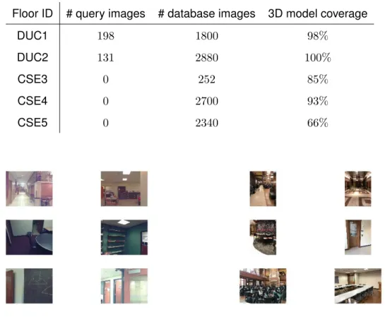
The InLoc dataset was designed to benchmark indoor long-term visual localization algo-rithms, it consists of a set of database images, a set of query images and a dense 3D model. Database images were collected from two different buildings, from now on re-ferred as DUC and CSE, from Washington university. The images from the DUC building were taken from two different floors and the images from the CSE building from three different floors and the original 3D coordinates are known for almost every pixel. Further information about how the 3D coordinates were obtained for the database images can be found in [53]. Query image were collected with an iPhone only from the DUC building. The dense 3D model of both buildings was obtained with a laser scanner. Tables 3.1 and 3.2 present further technical details. Some examples of query and database images from the dataset are shown in Figure 3.8.

Table 3.1.Dataset properties per image group.

# images Resolution (pixels) focal length (pixels)

Database images 9972 1600×1200 1430