ISSN 1750-4171
DEPARTMENT OF ECONOMICS
DISCUSSION PAPER SERIES
Human Capital and Spatial Heterogeneity
in the Iberian Countries’ Regional Growth
and Convergence
Catarina Cardoso
Eric J. Pentecost
WP 2011 - 04
Department of Economics
School of Business and Economics Loughborough University
Loughborough
LE11 3TU United Kingdom Tel: + 44 (0) 1509 222701 Fax: + 44 (0) 1509 223910
Human Capital and Spatial Heterogeneity in the Iberian Countries’ Regional Growth and Convergence
Catarina Cardoso and Eric J. Pentecost School of Business and Economics,
Loughborough University, Loughborough Leicestershire, LE11 3TU, UK August 2011 Abstract
Human capital is believed to be an important conditioning factor in explaining the convergence and the speed of convergence of regional economies, although it is usually excluded from the estimated models due to a lack of consistent data. In contrast this paper, using a newly constructed series on human capital at the NUTS III level for Portugal, evaluates the role of human capital on the speed of convergence using a spatial econometric methodology, for a sample of Iberian NUTS III regions over the period 1991-2006. This is the first study to consider human capital effects at the NUTS III level and the results show convergence, both absolute and conditional, occurs mainly in the peripheral group of regions, while human capital plays a positive role only in the club of the richest regions, in contrast with an insignificant effect in the periphery. There is also evidence of important regional spillovers between the regions and evidence of the importance of EU regional policy in enhancing the convergence of the NUTS III regions.
JEL Classification: C23, I21, O18, R11
1. Introduction
One of the key medium-term objectives of the European Union (EU) is economic and social cohesion, through reduced regional income disparities. If lower regional income disparities are to be achieved then regional economic convergence will need to occur. The notion of regional economic convergence has therefore generated a large empirical literature, stemming from Baumol (1986), Barro and Sala-i-Martin (1991), Button and Pentecost (1985) with more recent contributions surveyed in Islam (2003). This literature, however, is constrained in three dimensions. First, it is primarily concerned with convergence between NUTS I or NUTS II regions1, largely due to the data limitations at the NUTS III level, the finest level of regional disaggregation. Second, even at this relative aggregate level of regional data, there is no consistent data on human capital, and so strictly most of these studies potentially suffer from omitted variable bias. Thirdly, most studies measure regional convergence across the EU(12) or EU(15), which therefore typically include both the richest and some of the poorest regions of EU, thereby emphasizing the initial income divergences. A potentially more meaningful measure of convergence is that between regions in a sub-set of relatively similar countries. This would minimise any cultural or climatic differences between the regions and indicate to what extent there was sub-EU regional convergence, rather than sub-EU-level convergence. Given the relative lack of labour mobility across the EU and the very slow rates of economic convergence found across EU-wide studies, such local regional convergence may offer more practical and national political support for EU measures.
This paper addresses these three limitations of the existing literature by investigating the regional convergence between the 75 mainland NUTS III regions on the Iberian Peninsula between 1991 and 2006, over which period both countries were receiving significant structural fundsto catch-up with the other “Old EU” members. This is the first paper to study income convergence at the NUTS III level for Portugal and Spain2. In addition, it is also the first paper to use human capital in such a study at the NUTS III level, and to facilitate such analysis a human capital series for Portugal was computed from primary data (see Cardoso and Pentecost, 2011). Finally, by confining the analysis to the Iberian peninsula, the focus is on regional convergence, rather than convergence to some more distant, continental EU average. In addition,
1 NUTS stands for the European Commission’s Nomenclature of Statistical Territorial Units. 2Ramos
et al. (2010) study Spanish NUTS III regions. They find that the human capital effects on this set of regions are positive on productivity growth, but no evidence of human capital regional spillovers.
the use of spatial econometric methods allows for both spatial heterogeneity and sub-national regional spillover effects to be captured.
Our findings, based on beta-convergence measures, show that there are two regional clubs, which can be identified as the core and peripheral regions of the peninsula. We find that there has been a significant convergence of relative real per capita incomes in the peripheral regions, but not in the core regions, and that human capital is highly significant only in the core regions, perhaps reflecting the fact that human capital is only important above a certain level of economic development. There is also evidence of strong regional spillovers, as might be expected at the NUTS III level of disaggregation.
The structure of the paper is the following: Section 2 discusses the empirical β -convergence model and the human capital proxy used in this study. Section 3 presents the regional data and applies an exploratory spatial data analysis in order to describe the space dynamics, detect spatial autocorrelation and to identify potential spatial regimes. In Section 4, the spatial models and econometric techniques used to estimate the β-convergence model are presented and the results are discussed in Section 5. Section 6 concludes.
2. The β-convergence model
The standard convergence equation is derived from the augmented-Solow model dynamics around the steady-state [Mankiw et al. (1992)] and since human capital is one of the steady-state variables, this equation constitutes an empirical framework to estimate the effect of human capital on income per capita growth. It can be written as:
(1) where ln denotes a natural logarithm, the dependent variable gri t, is the GDP per capita growth rate relative to the regional average, yi,t1 is the lagged GDP per capita and Hi,t and ni,t are, respectively, the human capital level and the population growth
rate. ui,t stands for the idiosyncratic error term. In order to control for the business-cycle, both the lagged GDP per capita and the respective growth rate variables are expressed in deviation from the Iberian average. A negative-coefficient indicates convergence in the sense that the poorer is a region initially, the higher will be its
t i t i t i t i t i y H n g u gr, ln ,1 1ln( , )2ln( , ) ,
GDP per capita growth rate relative to the average of all the Iberian regions. The speed of convergence,, can be computed from (1) as ( T 1) 0
e
where e is the
base of natural logs and T is the time period, so in this case T =1 and ln(1). The time needed for the economies to reduce half of the deviation from the steady-state, the so-called half-life, is given by: ln(2)/ln(1).
The effect of human capital level (1) is expected to be positively significant because it enhances the region’s ability to adopt and create new technologies in the line with Benhabib and Spiegel (1994) and Romer (1990), respectively. 2 is expected to be negative in accordance with the theoretical predictions of the Solow growth model.
The most popular proxy for the human capital stock is the average years of education which can be defined as:
S i i t s t s AvEdu( ) ( , ) (2)where s stands for years of schooling and i(t,s)is the share of region’s i population with s years of schooling at time t. Although this proxy faces several limitations [Rogers (2008), Wößmann, (2003)], such as ignoring sources of human capital formation outside the education system and assuming that the formation of human capital per year of schooling is the same across levels of education, regardless the field of study and the quality of the education system, it has been largely applied in growth empirics due to data availability.
3. Exploratory Spatial Data Analysis
This regional data panel includes all continental Portuguese and Spanish regions, which number 28 and 47 respectively. Data on real GDP and population was collected from the respective country National Institute of Statistics (INE)’ Regional Accounts. Figures 1 and 2 display the quintile map obtained for the regional GDP per capita of the 75 NUTS III Iberian regions in the beginning and at the end of the period. The darkest regions represent the richest and are mostly located in the Basque Country and Cataluña, also including the Madrid region. The only Portuguese region that integrates with the richest group is the capital region, Grande Lisboa. The lightest
areas correspond to the poorest and contain only Portuguese regions.
There are some changes from 1991 to 2006. In Portugal the contrast between the richest and poorest regions was mainly a Coast/ Inland division in 1991 but this is not so striking in 2006. At the end of the period the quintile map suggests that most poor regions are located in the North while the richest seem to be in the South and then inside these two groups the regions at the coast tend to be better off than the inland regions. There was a significant decline in the relative position of the Portuguese second city region (Grande Porto) located in the North, which moved from the fourth to the second quintile over the period. In Spain there are also some changes over the time period of the sample, but the main features remain with a North and East rich club in contrast with a poor East and South. Apart from the capital region, Madrid, which is among the richest regions as expected, all the other regions located at the top of GDP per capita ranking are in the País Vasco (Basque Country) and Cataluña which are both in the Northeast and closer to the core European countries. The poorest regions are located in Andalucía, Extremadura and Galicia and they tend to remain poor over the period.
With regards to the regional human capital series, in the Portuguese case they are not available from any public source at this level of regional disaggregation so they need to be computed. The raw data was taken from Quadros de Pessoal (Personnel Records), a dataset that results from an annual compulsory questionnaire that every firm (except family business without employees) must answer and is applied by the Strategic and Planning Office (GEP) of the Portuguese Ministry of Labour and Social Solidarity (MTSS). The data provided by this institution are the number of workers in each region according to the level of qualification. The dataset excludes the public sector and the self-employed workers. An interpolation was done for the year 2001, since there is no data available for this particular year (see Cardoso and Pentecost, 2011).
In contrast with Portugal, data on Spanish human capital at the NUTS III level of regional disaggregation is available from Fundación Bancaja-IVIE (Instituto Valenciano de Investigaciones Económicas). For each NUTS III region, the IVIE human capital dataset provides the average years of schooling of the total workers employed3 and also the number per level of education in each of the following
3 Población Ocupada
sectors: agriculture, building, energy, industry, trade services and non-trade services. The latter is used as a proxy for the public sector. Since the education proxy estimated for Portugal excludes the public sector, the workers in the non-trade services have been removed from the computation of the average years of education for the Spanish regions in order to make a more consistent comparison of the results obtained for both countries. In Spain, the compulsory schooling correspond to 8 years of lower secondary school, one year less than in Portugal. In 1991 the average years of education in Portugal was 6, in Spain 7.7, and they increase to 8.5 and 10.2, respectively, at the end of the period.
The spatial distribution of human capital as proxied by the average years of education in the Iberian countries continental regions can be seen in Figures 3 and 4. The darkest regions are the richest and the lightest correspond to the poorest. It is striking that over the period none of the Portuguese regions match the group of the richest, which reflects the low levels of human capital in Portugal relative to Spain. Among the first and second quintile are all the Portuguese regions apart from the capital (Grande Lisboa). In Spain the regions with a higher level of human capital are Madrid, Cataluña and Basque Country which are simultaneously those with a higher GDP per capita.
The quintile maps of both GDP per capita and human capital suggest some clears spatial patterns. The analysis will proceed with a more formal detection of spatial autocorrelation in the variables of interest. Global spatial autocorrelation for each variable is measured through the Moran’s I statistic [Anselin (1995)]:
t t t t t z z Wz z S n I ' ' 0 (3)
were n is the number of observations, zt is the vector of observations for year t in deviation from the mean, W is the spatial weights matrix, S0 is the scaling constant, this is the sum of all spatial elements of W. Wztis the vector of spatially weighted averages of neighbouring values, this is the spatially lagged vector. A positive value of the Moran’s I indicates positive spatial autocorrelation and a negative indicates negative spatial autocorrelation. The spatial weights matrix W is a square matrix with N rows/ columns that correspond to the number of regions and captures their spatial
interaction. The diagonal consists of zeros and each wij defines the way a region i is connected with the region j. Here the contiguity-based spatial weights matrix is applied, which is constructed by assigning a weight of 1 to all j regions that are contiguous to i, and zero to all the others. This relies on the regions’ depiction on the map.
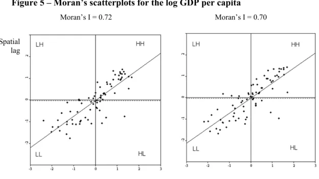
Moran’s scatter plot plots the variable of interest on the x-axis (zt) against the respective spatial lag on y-axis (Wzt). The spatial lag of a regional variable is the
respective value in the neighbouring regions. A Rook-contiguity matrix is applied in this section, so the spatial lag of the variable of interest is the average of the values in the regions that have a common boundary with the region of interest. The four quadrants that result from the scatter plot correspond to four types of local spatial association between a region and the respective neighbours:
1) HH – a region with a high value, this is above the mean, is surrounded by regions that have high values as well;
2) HL – a region with a high value surrounded by regions with low values, this is below the mean;
3) LL – a region with a low value surrounded by regions with low values as well; 4) LH – a region with a low value surrounded by regions with high values.
The quadrants HH and LL refer to positive spatial correlation, which indicates clustering of similar values. In contrast, the quadrants LH and HL represent negative spatial autocorrelation, this is spatial clustering of dissimilar values. The Moran’s scatter plot slope is the Moran’s I statistic for the variable of interest and since the variables are standardized the scatter plots are comparable over time.
Figure 5 displays the Moran’s scatter plots of the regional GDP per capita. The spatial lag of this variable is the average regional GDP per capita of the neighbouring regions. As can be seen the quadrants are relatively stable over time. Most regions are located in quadrants HH, rich regions surrounded by rich regions, and LL, poor regions that have poor neighbours. The rich regions in the quadrant HH are the Spanish regions located in the Basque country, Cataluña and the capital region Madrid. Almost every Portuguese regions and the Spanish regions that integrate Galicia and Extremadura are found in the LL quadrant.
The atypical regions are located in the quadrants LH, these are poor regions surrounded by rich neighbours, and HL, which are rich regions that have poor
neighbours. In the HL quadrant are located the Portuguese richest regions, these are the capital region, Grande Lisboa followed by Alentejo Litoral and Grande Porto. From 1991 to 2006 two Spanish regions joined this group, Almería and Huelva, which are located in the Mediterranean coast and have developed a strong tourist sector. Both in 1991 and 2006 most of the regions are located in either quadrant HH or LL which suggests two spatial regimes.
Figure 6 displays the Moran’s scatter plots of the log of regional human capital as proxied by education in 1991 and 2006. As shown the quadrants are relatively stable over time. Similar to regional GDP per capita, most regions are located in quadrants HH, rich regions surrounded by rich regions, and LL, poor regions that have poor neighbours. The rich regions in the quadrant HH are all Spanish. All the Portuguese regions apart from the capital are located in the LL quadrant. In 1991 there was only one Spanish region in the former quadrant, Ourense, but due to a significant improvement in 2006 this region was already in the quadrant of the rich regions with poor neighbours (HL), where the Portuguese capital region Grande Lisboa is located together with some Spanish regions located on the border such as Salamanca, Badajoz and Huelva.
The exploratory spatial data analysis suggests significant positive global spatial correlation in the regional GDP per capita and human capital. The rich regions are close to each other and they tend to remain in the same group over time. This evidence of spatial clusters of high and low values for both GDP per capita and human capital can be interpreted as different spatial regimes and suggests spatial heterogeneity. There is spatial heterogeneity when the economic relation among the variables is not stable across space. These spatial regimes can be seen as “convergence clubs” and the convergence process might differ according to the “club”. A convergence club can be defined as a group of regions that subject to some initial sorting based on their structural characteristics converge within their own group. The concept is based on the idea that multiple, locally stable, steady-state equilibrium points are possible [Azariadis and Drazen (1990) and Durlauf and Johnson (1995)]. The particular equilibrium reached by a region depends on the group to which it belongs, according to the respective initial conditions. The clubs are linked with spatial heterogeneity which must be taken into account otherwise the β -convergence model estimation is unreliable.
In this section convergence clubs within the Iberian Peninsula will be identified following the procedure of Ertur et al. (2006) who used the Moran’s scatterplot to determine four spatial clubs among 138 EU15 regions: clusters of rich regions, clusters of poor regions and the two atypical groups formed by rich regions surrounded by poor and the reverse. These atypical groups are dropped out of the sample, since they are insufficient in number to form another regime, and so only the rich (Core) and poor (Periphery) clubs are considered.
Moran’s scatter plot for the initial GDP per capita in Figure 5 showed that most of the Iberian regions are located either in quadrant HH or LL which can therefore be considered as two spatial clubs: the Core, which corresponds roughly to the East of the Iberian Peninsula, and the Periphery, which is mainly constituted by regions located on the West. The Core group is closer to the main EU countries and the Peripheral group is further. The atypical regions which were notoriously in the quadrant HL are the richest Portuguese regions (Grande Lisboa, Grande Porto and Alentejo Litoral) and the Spanish region of Huelva. They are dropped since the small number of observations does not allow proceed to the estimations for this third spatial regime. The other atypical regions are not far from the main spatial regimes (HH or LL) so they were allocated to the club which they are closer to. A different set of coefficients must be estimated for each club since the convergence process might be quite different across the regimes. Figure 6 illustrates the two convergence clubs.
4. Spatial models and the econometric methodology
There are two main spatial dependence models: Spatial Lag Model (SLM) or the Spatial Error Model (SEM) (Anselin, 1988; and Rey and Le Gallo, 2009). In the SLM the spatial autocorrelation is modeled through the use of the spatially lagged dependent variable, which is added to the right-hand side of the regression specification, whereas in the SEM it is the error term which captures the spatial structure. In formal terms the SLM is:
WY X
Y (4)
where
Y
is the vector of regional dependent variable, X is the matrix of explanatory variables, is the spatial autoregressive parameter and W is the standardised spatial weights matrix (where the elements of each row sum up to one), that captures thespatial interaction between regions andis the well-behaved error term such that, 2
(0, )
N I
.
In contrast the SEM is represented as: the error term u adopts a spatial structure which means that, this is:
u X Y Wu u (5) (6) where Y is again the vector of regional dependent variable, X the matrix of explanatory variables, W is the standardised spatial weights matrix, and is the normally distributed error term, but now u is the spatially correlated error, showing that externalities now only come from the shocks andis the autoregressive error coefficient.
The choice between the two models is made according to the Lagrange Multiplier (LM) test statistics. The LM-Lag and Robust LM-Lag favour the spatial lag model as the alternative while the LM-Error and Robust LM-Error suggest the spatial error model as the appropriate specification. The LM statistics are distributed as a 2with one degree of freedom and the robust tests should only be considered if the respective standard versions are significant. If it is not the case, the properties of the robust tests may no longer hold. When both the LM-lag and the LM-error are significant but only the robust LM-lag is significant, the spatial lag model is chosen as the appropriate model. In the rare case that both are highly significant, the model with a largest value for the test statistic is selected but in this case some caution is needed. Both models are estimated for the panel data set by maximum likelihood procedures under the normality assumption.
The conditional β-convergence model should be specified taking into account the two convergence clubs previously identified [see Ramajo et al. (2008)]. This is:
, , 1 , 1 1 , 1 , 2 , 2 , , ln ln ln( ) ln( ) ln( ) ln( ) (7) i t C C P P c C i t P P i t C C i t P P i t C C i t P P i t i t gr D D D y D y D H D H D n g D n g u
where the subscripts C and P stand for the Core and Periphery club, respectively. The dummy D takes the value 1 when the region belongs to that club and zero otherwise. In this specification the spatial effects are assumed to be identical in both clubs and all
the regions are still interacting in spatial terms with each other. This is the model estimated in the next subsection following the spatial fixed effects panel data model proposed by Elhorst (2009).
Panel data methods are the only way to obtain consistent estimates of a conditional convergence equation (Temple, 1999) and the main advantages over cross-section include the possibility of taking into account the omitted variables and endogeneity problems. Since the unobserved individual specific effects are likely to be correlated with the other explanatory variables, the fixed effects estimator is more appropriate than the random-effects. Even though the presence of the lag of the dependent variable in the convergence equation invalidates the strict exogeneity assumption and therefore the Generalized Method of Moments (GMM) is the most appropriate estimator for the convergence equations (Bond et al., 2001). Estimating a spatial model through GMM, however, has some disadvantages such as finding estimators for the spatial autoregressive parameter () or the autoregressive error coefficient ( ) that are outside the parameter space (Elhorst, 2009). Thus the convergence equation (7) is estimated using the spatial fixed effects model and the maximum-likelihood procedures.
5. Results
Table 1 displays the results for the absolute convergence model. Looking at the OLS results, the robust LM-error statistics suggest the Spatial Error Model as the most appropriate. The initial GDP per capita coefficient is only negatively significant in the periphery group and this is confirmed by the fixed effects Spatial Error Model (SEM-FE) suggesting that convergence is a phenomenon that concerns only this spatial club. The convergence rate of 3.05% per annum implies 23 years are needed to reduce half of the gap towards the common steady-state, which as expected, is slightly lower than the 29 years of Ertur et al (2006) for the periphery club within the EU15 NUTS II regions. The statistical significance of the autoregressive error coefficient (λ) confirms the SEM as appropriate and suggests that a random shock in an Iberian region propagates to all other regions, although in the context of absolute convergence, the spatial autocorrelation coefficient can work as a proxy for omitted variables (Le Gallo and Ertur, 2003).
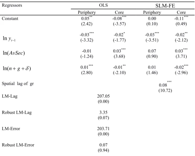
alternative measures of human capital, proxied by the average level of education (AvEdu), the average years of secondary education (AvSec) and the average years of Tertiary education (AvTer), respectively. In every case the OLS results suggest convergence, with a positive, significant coefficient on the measure of human capital in the core. The LM-Lag and the Robust LM-Lag tests, however, suggest that the null hypothesis of no spatial serial correlation is rejected in favour of the SLM with fixed effects (SLM-FE).
The SLM-FE results show that human capital proxies are all statistically significant in the core regions, but not in the peripheral regions, and with the average years of schooling and average years of secondary education seemingly more important than average years in tertiary education, given the larger coefficients (0.03 compared to 0.01). The concentration of the positive effect of human capital in the developed regions suggests two things: first, that a certain level of economic development is required in order to obtain gains from the investment in education; and second, that human capital is an important conditional variable in the convergence growth regression, despite its frequent exclusion, albeit due to a lack of data, from most studies.
The SLM-FE in Tables 2 to 4 also show significant convergence in both periphery and core regions, with the exception of the model including the average education proxy, where the coefficient is insignificant for the core, but of the correct sign, although as expected, convergence is stronger for the peripheral club. The speed of convergence, however, even for the peripheral club is only between 2% and 3% per annum, depending on the human capital proxy used. Convergence is fastest when the secondary education proxy is used for human capital (Table 3). The peripheral regions convergence is therefore very slow with at best 23 years required for half of the gap towards the steady-state, which is slightly quicker than the 29 years reported in Ertur et al (2006), using NUTS II data and EU15 regions. In Tables 2 and 4 when average years of schooling or average years in tertiary education are used as proxies for human capital, the half-life is 34 years, which can be interpreted as showing that secondary education is the most important kind of education for the regional convergence process.
In each of Tables 2 to 4 the coefficient on the spatial lag of GDP growth () is positive and highly significant at the one percent level, suggesting important regional
spillovers at the NUTS III level of regional disaggregation..
Two further experiments were undertaken to test the robustness of these results when other conditional variables – often used in NUTS level II studies – are added to the model. The addition of a regional policy dummy, which is one for all regions receiving structural or cohesion funds and zero for the others, is never found to be significant, however, its inclusion increases the speed of convergence in the periphery to around 4% per annum and therefore it reduces the time needed to reduce half of the gap towards the steady-state to about 17 years. This is in accordance with the results of Mohl and Hagan (2010), who using a conditional -convergence model to study the effects of structural funds on EU regional growth, find that the speed of convergence increases when the structural funds are added to the growth equation, although, the total funds allocated have an insignificant (negative) effect on regional growth. In the current NUTS III level study regional policy also reinforces the effect of human capital on the core regions’ growth and the coefficient on the regional spillovers increases significantly from 0.08 to 0.38. This suggests that one of the main benefits of regional policy at the NUTS III level is in generating spillover benefits rather than just to raise income in the specific region to which the funds are directed.
The second addition to the model was to include a variable representing the share of gross added value in agriculture, which is found to be significant in every case, although in this case reliance is placed on the OLS results because the spatial models cannot be distinguished. The coefficient on gross value added in agriculture is much larger in the periphery than in the core regions, although it has a positive sign rather than a negative sign, as expected. A negative sign was expected since regional agricultural output may serve as a proxy for a lack of regional human capital at the NUTS III level. The simple partial correlation coefficient between the regional human capital and the regional gross value added in agriculture was (-0.59) and statistically significant at the five per cent level, provides evidence of this possibility. The positive sign on the gross added value in agriculture may also reflect the fact that the most agricultural intensive regions grow faster because they are poorer. This extension of the model does show, however, that the signs and significance of the other conditional variables are robust in that the magnitudes of the -coefficients and human capital coefficients are not affected by the inclusion of this additional variable.
6. Conclusions
The Exploratory Spatial Data Analysis of the Iberian NUTS III level regions dataset identified both spatial dependence and spatial regimes. Spatial regimes can be seen as different convergence clubs and there are significant differences across them. Convergence, both absolute and conditional, occurs mainly in the periphery group. This finding is in accordance with previous studies for the EU15 NUTS II regions which found that convergence is a phenomenon that mainly concerns the poorest regions club [Ertur et al. (2006), Dall’Erba and Le Gallo (2008)].
The effect of the conditional variables on growth also varies across the spatial regimes. Human capital proxied by the average years of total, secondary and higher education plays a positive and significant role in the Core club, but not in the Periphery, which suggests that a certain level of economic development is required to achieve a positive effect of human capital. The effect of secondary education on the Core regions’ growth is stronger than that of higher education. The fact that the Iberian regions tend to be technological “followers” might explain the lower effect of higher education in comparison with the secondary level since the effect of higher levels of education on growth increases as the or regions become closer to the technological frontier (Vandenbussche et al., 2006). Important regional spillovers were detected which indicates that the growth of a region depends not only on its own conditions but also on the neighbour’s dynamics. The channels through which these regional spillovers operate constitute a future research direction.
References
Abreu, M., de Groot, H. and Florax, R. (2005), “Space and Growth: a Survey of Empirical Evidence and Methods”, Région et Développement, 21, pp.13-44. Anselin (1988), Spatial Econometrics: Methods and Models, Klwer, Dordrecht, The
Netherlands.
Anselin (2003), “Spatial Externalities, Spatial Multipliers and Spatial Econometrics”, International Regional Science Review, 26, pp. 156-166.
Anselin, L. (2005), “Exploring Spatial Data with GeoDa: A Workbook”, Spatial Analysis Laboratory, Department of Geography, University of Illinois, Urban-Champaign.
Anselin, L., Syabri, I. and Kho, Y. (2006), “GeoDa, an Introduction to Spatial Analysis”, Geographical Analysis, 38(1), pp. 5-22.
Arbia, G., Batisit, M. and Di Vaio, G. (2010), “Institutions, and geography: Empirical Test of Spatial Growth Models for European Regions”, Economic Modelling, 27(1), pp. 12-21.
Azariadis, C. and Drazen, A. (1990), “Thresholds Externalities in Economic Development”, Quarterly Journal of Economics, 105(2), pp. 501-526.
Barro, R. and Sala-i-Martin, X. (1992), “Convergence”, Journal of Political Economy, 100(2), pp. 223.
Baumol, W.J. (1986), “Productivity Growth, Convergence and Welfare: What the Data Show,” American Economic Review, 76, pp. 1075-1085.
Benhabib, J. and Spiegel, M. (1994), “The Role of Human Capital in Economic Development: Evidence from Aggregate Cross-country Data”, Journal of Monetary Economics, 34(2), pp. 143-173.
Bond, S., Hoeffler, A. and Temple, J. (2001), “GMM Estimation of Empirical Growth
Models”, CEPR Discussion Papers No. 3048.
Button, K.J. and Pentecost. E.J. (1995), “Testing for Convergence of the EU Regional Economies,” Economic Inquiry, pp. 664-671.
Cardoso, C. and Pentecost, E.J. (2011), “Regional Growth and Convergence: The Role Human Capital in Portuguese Regions,” Loughborough University, EconomicsDiscussion Paper No. 2011-03.
Dall’Erba, S. and Le Gallo, J. (2008), “Regional Convergence and the Impact of European Structural Funds over 1989-1999: A Spatial Econometric Analysis”, Papers in Regional Science, 87 (2), pp. 219-244.
Durlauf, S. and Johnson, P. (1995), “Multiple Regimes and Cross-Country Growth Behaviour”, Journal of Applied Econometrics, 10, pp. 365-84.
Elhorst, P. (2009), “Spatial Panel Data Models” in Fisher, M. and Getis, A. (ed.), Handbook of Applied Spatial Analysis, Springer, Berlin.
Ertur, C., Le Gallo, J. and Baumont, C. (2006), “The European Regional Convergence Process, 1980-1995: Do Spatial Regimes and Spatial Dependence Matter?” International Regional Science Review, 29(3), pp. 3-34.
Le Gallo, J. and Ertur, C. (2003), “Exploratory Spatial Data Analysis of the Distribution of Regional per capita GDP in Europe, 1980-1995”, Papers in Regional Science, 82, pp. 175-201.
Lόpez-Bazo E., Vayá E. and Artís, M. (2004), “Regional Externalities and Growth: Evidence from European Regions”, Journal Regional Science, 44 (1), pp. 43-73.
Mankiw, G., Romer, D. and Weil, D. (1992), “A Contribution to the Empirics of the Economic Growth”, Quarterly Journal of Economics, 107 (2), pp. 407-37.
Mohl, P. and Hagan, T. (2010), “Do Structural Funds Promote Regional Growth? New Evidence from Various Panel Data Approaches,’ Regional Science and Urban Economics, 40, pp. 353-365.
Ramajo, J., Márquez, M., Hewings, G. and Salinas, M. (2008), “Spatial Heterogeneity and Interregional Spillovers in the European Union: Do Cohesion Policies Encourage Convergence across Regions?” European Economic Review, 52, pp. 551-567.
Ramos, R., Suriñach, J. and Artís, M. (2010), “Human Capital Spillovers, Productivity and Regional Convergence in Spain”, Papers in Regional Science, 89, pp. 435-446.
Rey, S. and Le Gallo, J. (2009), “Spatial Analysis of Economic Convergence” in Mills, T. and Patterson, K. (ed.), Palgrave Handbook of Econometrics, Vol. 2, Palgrave Macmillan, London, UK.
Rogers, M. (2008), “Directly Unproductive Schooling: How Country Characteristics Affect the Impact of Schooling on Growth”, European Economic Review, 52(2), pp. 356-85.
Romer, P. (1990), “Endogenous Technological Change”, Journal of Political Economy, October, S71-S102.
Temple, J. (1999), “The New Growth Evidence”, Journal of Economic Literature, 37(1), pp. 112-156.
Wößmann, L. (2003), “Specifying Human Capital”, Journal of Economic Surveys, 17(3), pp. 239-270.
Vandenbussche, J., Aghion, P. and Meghir, C. (2006), “Growth, Distance to Frontier and Composition of Human Capital”, Journal of Economic Growth, 11(2), pp. 97-127.
Figure 1 – Regional GDP per capita 1991 quintile map
Figure 3 – Regional Human Capital 1991 quintile map
Figure 5 – Moran’s scatterplots for the log GDP per capita
Figure 6 - Moran’s scatterplots for the log Average Education
ln GDP per capita 1991 Spatial lag Moran’s I = 0.72 ln GDP per capita 2006 Moran’s I = 0.70
ln Average Years Education 1991 Spatial
lag
Moran’s I = 0.78 Moran’s I = 0.66
Table 1 – Absolute convergence model in Iberia
Dependent variable: GDP per capita growth rate (gr)
Regressors OLS SEM-FE
Periphery Core Periphery Core
Constant -0.01* (-1.71) -0.00 (-0.17) -0.01* (-1.83) -0.00 (0.87) -0.03*** (-4.31) -0.00 (-0.55) -0.03*** (-4.27) -0.01 (-0.72) Autoregressive error ( λ) -0.09*** (12.42) LM-Lag 222.06 (0.00) Robust LM-Lag 0.86 (0.35) LM-Error 226.73 (0.00) Robust LM-Error 5.53 (0.02)
Notes: t and z-statistics (OLS and SEM, respectively) in brackets, except for the diagnostic tests whose p-values are reported. ***, ** and * indicate statistical significance at 1%, 5% level and 10% level.
1 lnyt
Table 2 – Convergence conditional on human capital in Iberia
Dependent variable: GDP per capita growth rate (gr)
Regressors OLS SLM-FE Periphery Core Periphery Core
Constant 0.08 (0.55) -0.16*** (-4.11) 0.04 (1.62) -0.12*** (-3.41) -0.02*** (-2.84) -0.02** (-2.13) -0.02*** (-2.85) -0.01 (-1.60) -0.02* (-1.89) 0.06 *** (3.90) (-0.92)-0.01 0.03 *** (2.84) 0.01*** (2.73) -0.01 ** (-2.07) 0.01 ** (2.10) -0.01 ** (-2.54) Spatial lag of gr 0.09*** (13.50) LM-Lag 204.38 (0.00) Robust LM-Lag 3.81 (0.05) LM-Error 200.57 (0.00) Robust LM-Error (0.00) (0.98)
Notes: t and z-statistics (OLS and SEM, respectively) in brackets, except for the diagnostic tests whose p-values are reported. ***, ** and * indicate statistical significance at 1%, 5% level and 10% level.
1 lnyt ) ln(AvEdu ) ln(ng
Table 3 – Convergence conditional on secondary education in Iberia
Dependent variable: GDP per capita growth rate (gr)
Regressors OLS SLM-FE
Periphery Core Periphery Core
Constant 0.05** (2.42) -0.08*** (-3.57) 0.00 (0.10) -0.11*** (0.49) -0.03*** (-3.32) -0.02* (-1.77) -0.03*** (-3.51) -0.02** (-2.12) -0.01 (-1.24) 0.03 *** (3.68) (0.90) 0.07 0.03 *** (3.71) 0.01*** (2.80) -0.01 ** (-2.10) (1.46)0.01 -0.02 *** (-2.96) Spatial lag of gr 0.08*** (10.72) LM-Lag 207.05 (0.00) Robust LM-Lag 3.35 (0.07) LM-Error 203.71 (0.00) Robust LM-Error 0.07 (0.94)
Notes: t and z-statistics (OLS and SEM, respectively) in brackets, except for the diagnostic tests whose p-values are reported. ***, ** and * indicate statistical significance at 1%, 5% level and 10% level.
1 lnyt ) ln(AvSec ) ln(ng
Table 4 – Convergence conditional on higher (tertiary) education in Iberia
Dependent variable: GDP per capita growth rate (gr)
Regressors OLS SLM-FE
Periphery Core Periphery Core
Constant 0.03** (2.15) -0.04** (-2.27) 0.01 (0.88) -0.06*** (0.49) -0.02*** (2.15) -0.02** (2.15) -0.02** (2.15) -0.01* (2.15) -0.01** (-2.41) 0.01 *** (3.77) (-1.06) -0.00 0.01 *** (2.96) 0.01*** (2.67) -0.01 ** (-2.02) -0.02 *** (-3.06) 0.08 *** (10.71) Spatial lag of gr 0.08*** (10.72) LM-Lag 204.11 (0.00) Robust LM-Lag 6.04 (0.01) LM-Error 198.27 (0.00) Robust LM-Error 0.20 (0.65)
Notes: t and z-statistics (OLS and SEM, respectively) in brackets, except for the diagnostic tests whose p-values are reported. ***, ** and * indicate statistical significance at 1%, 5% level and 10% level.
1 lnyt ) ln(AvTer ) ln(ng