DOI 10.1007/s10687-016-0255-3
Approximation of high quantiles from intermediate
quantiles
Cees de Valk1
Received: 27 May 2013 / Revised: 4 March 2016 / Accepted: 28 April 2016 / Published online: 27 May 2016
© The Author(s) 2016. This article is published with open access at Springerlink.com
Abstract Motivated by applications requiring quantile estimates for very small prob-abilities of exceedancepn1/n, this article addresses estimation of high quantiles forpnsatisfyingpn ∈ [n−τ2, n−τ1]for someτ1>1 andτ2 > τ1. For this purpose, the tail regularity assumption logU◦exp∈ERV (withUthe left-continuous inverse of 1/(1−F ), andERV the extended regularly varying functions) is explored as an alternative to the classical regularity assumptionU ∈ ERV (corresponding to the Generalised Pareto tail limit). Motivation for the alternative regularity assumption is provided, and it is shown to be equivalent to a limit relation for the logarithm of the survival function, the log-GW tail limit, which generalises the GW (Generalised Weibull) tail limit, a generalisation of the Weibull tail limit. The domain of attrac-tion is described, and convergence results are presented for quantile approximaattrac-tion and for a simple quantile estimator based on the log-GW tail. Simulations are pre-sented, and advantages and limitations of log-GW-based estimation of high quantiles are indicated.
Keywords Extreme value theory·Quantile estimation·High quantile·Generalised Weibull tail limit·log-GW tail limit·Weibull tail limit·Extended regular variation AMS 2000 Subject Classifications 60G70·62G32·26A12·26A48
Cees de Valk
1 Introduction
An important application of extreme value theory is the estimation of tail quantiles. Theoretical analysis usually addresses tail quantile estimation fromnindependent random variables{X1, ..., Xn}with common distribution functionF, and considers the asymptotic properties of estimators asn → ∞. Of particular interest arehigh quantiles, exceeded with probabilities pn = O(1/n); see e.g. Weissman (1978), Dekkers et al. (1989), de Haan and Rootz´en (1993) and for dependent random variables, Drees (2003).
LetX1,n ≤X2,n ≤...≤ Xn,nbe the order statistics derived from{X1, ..., , Xn}, and letUdenote the left-continuous inverse of 1/(1−F )on(1,∞). Theintermediate quantileU (n/kn), with the sequence(kn)satisfying
kn∈ {1, .., n} ∀n∈N, kn/n→0 and kn→ ∞, (1.1) is under certain additional conditions estimated consistently by the intermediate order statisticXn−kn+1,n(e.g.de Haan and Ferreira (2006), Theorem 2.4.1). In
con-trast, the expected number of data points exceeding a high quantile is eventually bounded. A high quantile estimator can therefore not be expected to converge with-out some form of regularity of the tail, allowing it to be derived from intermediate order statistics.
The classical regularity assumption on the upper tail of the distribution function
F is often expressed as a condition onU; it requires that a positive functionwand a non-constant functionϕexist such that
lim t→∞
U (tλ)−U (t)
w(t) =ϕ(λ) ∀λ∈Cϕ, (1.2)
withCϕthe continuity points ofϕin(0,∞). As the limiting functionϕis continuous (e.g.de Haan and Ferreira (2006), Theorem 1.1.3), U satisfying (1.2) is extended regularly varying (seee.g.Appendix B2 of de Haan and Ferreira (2006), or Chapter 3 of Bingham et al. (1987)). Therefore, wcan be chosen to be regularly varying and (sinceUis nondecreasing) such that
ϕ=hγ (1.3)
for some realγ with for all positiveλ,
hγ(λ):=1λt
γ−1dt, (1.4)
which isγ−1(λγ−1)ifγ =0 and logλifγ =0; (1.2) with (1.3) is equivalent to a Generalised Pareto (GP) tail limit for the survival function (e.g.de Haan and Ferreira (2006), Theorem 1.1.2). In (1.2), the limit on the right-hand side was left unspecified in order to stress the nonparametric nature of the classical regularity assumption, which makes it particularly attractive from the point of view of applications.
When referring to (1.2), we will writeU ∈ERV, withERV the extended regu-larly varying functions1. We will writeU ∈ERVS to specify that in addition, (1.3) holds withγ ∈S ⊂R, andU ∈ERV{γ}(w)for (1.2) and (1.3) with a particularγ and positivew. We will apply the same notational conventions when a limit relation of the form (1.2) applies to a nondecreasing function other thanU. For a regularly varying functiong(e.g.Bingham et al. (1987)), we will writeg ∈RV, org∈ RVS to specify that limt→∞g(tλ)/g(t)=λαfor allλ >0 for someα∈S⊂R.
It has been known for long that existence of the limit (1.2) alone is of limited value for approximation of a high quantileU (1/pn)withpn = O(1/n)from an intermediate quantileU (n/kn)with(kn)as in (1.1), sinceλn := kn/(npn) → ∞ asn → ∞. Usually, additional assumptions on the rate of convergence in (1.2) are introduced for this purpose, such as (strong) second-order extended regular variation (de Haan and Stadtm¨uller (1996), de Haan and Ferreira (2006)), the Hall class (Hall (1982)), or conditions (1.5) and (1.6) of de Haan and Rootz´en (1993).
In this article, a different approach is explored: instead of strengthening (1.2), we will look for an alternative regularity assumption specifically to approximate certain high quantiles from intermediate quantiles, and by extension, to estimate such high quantiles. The quantiles we will focus on are very high quantiles corresponding to probabilities of exceedance(pn)satisfying
pn∈ [n−τ2, n−τ1] for some τ1>1, τ2> τ1, (1.5) without excluding that the approximation may also be suitable for less rapidly van-ishing(pn). This choice is motivated by applications requiring quantile estimates for probabilities of exceedancepnsatisfyingpnn1, such as flood hazard assessment (de Haan (1990)), design criteria on wind, waves and currents for offshore structures (ISO (2005), paragraph A.5.7), seismic hazard assessment (Adams and Atkinson (2003)) and analysis of bank operational risk (Cope et al. (2009)). In such applica-tions, one would want an estimator forU (1/pn)which converges in a meaningful sense even whenpnn → 0 asn → ∞. However, the latter condition is difficult to handle in its full generality. Therefore, we will narrow the focus to(pn)satisfying (1.5). Moreover, we will try to find an estimator which forpn =n−τ converges (in some yet-to-be-defined sense) uniformly inτ ∈ [1, T]for everyT > 1. In practi-cal terms, this means that if the assumptions for convergence are satisfied, then an estimate of a quantile exceeded with a probability of, say, 0.01 can be extended to an estimate of the quantile exceeded with a probability of 0.0001 without seriously stretching the assumptions2, as these probabilities differ only a factor of two in terms ofτ. Such flexibility is important in applications, becausepnis generally based on social and economic considerations, without regard for the feasibility of estimating
U (1/pn).
For convenience, we will assume throughout thatU (∞):=limt→∞U (t) >1.
1Ignoring that as an assumption, (1.2) is formally weaker thanU∈ERV; but sinceUis nondecreasing, we know thatCϕ=R+, so the difference is immaterial.
2 An alternative regularity condition
The alternative regularity assumption on the upper tail ofF proposed for estimation of a very high quantileU (1/pn)with(pn)satisfying (1.5) is
logq∈ERV (2.1)
with
q:=U◦exp. (2.2)
(2.1) is of the same nonparametric form as the classical regularity assumption (1.2), but withU replaced by logU◦exp. Therefore, it implies that for some realθ
and positive functiong, lim y→∞
logq(yλ)−logq(y)
g(y) =hθ(λ) ∀λ >0. (2.3)
To see the relevance of (2.1) for approximation of a very high quan-tile q(−logpn) = U (1/pn) with (pn) satisfying (1.5) from an interme-diate quantile q(log(n/kn)) = U (n/kn), assume that in addition to (1.1), lim supn→∞logkn/logn < 1. This ensures that −logpn = O(log(n/kn)) as
n→ ∞, and since convergence in (2.3) is locally uniform inλ > 0 (e.g.Bingham et al. (1987), Theorem 3.1.16), it implies
lim n→∞ logU (1/pn)−logU (n/kn) g(log(n/kn)) − hθ log(1/pn) log(n/kn) =0.
The limit relation (2.3) can be reformulated in terms of the survival function: Theorem 1 The limit relation (2.3) for some positive function g and real θ is equivalent to
lim y→∞
log(1−F (q(y)exg(y)))
y = −h
−1
θ (x) ∀x∈hθ(R+), (2.4)
Proof Equivalence of (2.3) and (2.4) is implied by Lemma 1.1.1 in de Haan and Ferreira (2006).
The pair (2.3) and (2.4) of equivalent limits can be seen as the analogue for logq
of (1.2) withϕ=hγ and the equivalent GP limit for the survival function lim
t→∞t (1−F (xw(t)+U (t)))=1/ h
−1
γ (x) ∀x∈hγ(R+) (2.5) (e.g. de Haan and Ferreira (2006), Theorem 1.1.2). It is important to realise that convergence of a log-ratio of probabilities as in (2.4) is a much weaker notion than convergence of a ratio of probabilities as in the GP limit (2.5). This difference reflects precisely the difference in extrapolation range between (2.3) and (1.2): when extrap-olating over a longer range, larger errors should be expected in principle, unless additional assumptions apply.
To illustrate that condition (2.1) is a natural assumption, Proposition 1 below shows how it may arise in the context of a GP tail limit (1.2) with (1.3) and the GP quantile approximation
˜
Ut(z):=U (t)+hγ(z/t)w(t) (2.6)
withwandγas in (1.2) and (1.3). Proposition 1 LetU ∈ERV{γ}(w). (a) Ifγ >0, then lim t→∞ logU˜t(tλ)−logU (tλ) logU (tλ)−logU (t) =0 ∀λ >1 (2.7) and logq∈ERV{1}. (b) Ifγ =0and lim t→∞ ˜ Ut(tλ)−U (tλ) U (tλ)−U (t) =0 ∀λ >1, (2.8) then
q∈ERV{1} and logq∈ERV{0}(1).
Proof The proof is found in Subsection7.1.
For distribution functions in the domain of attraction of the GP tail limit, Proposi-tion 1 shows that the condiProposi-tion (2.1) must hold ifγ >0; ifγ =0, it is a necessary condition for convergence of the relative error in the GP approximation in the sense of (2.8)3.
Proposition 1 also provides some basic insight into the strengths and limitations of the GP quantile approximation (2.6) for very high quantiles. Ifγ > 0, there is no problem; the notion of convergence in (2.7) may be weak, but can be considered appropriate for these heavy-tailed distribution functions. However, ifγ =0 and (2.8) holds, then necessarily,q ∈ ERV{1}, which is a restrictive condition. For example,
for the normal distribution,q∈ERV{1/2}, so (2.8) cannot hold.
In analogy to (1.2), a natural generalisation ofq∈ ERV{1}would beq ∈ERV,
so for some realθand some positive functiong, lim
y→∞
q(yλ)−q(y)
g(y) =hθ(λ) ∀λ >0. (2.9)
By a slight modification of Theorem 1, (2.9) is equivalent to lim
y→∞
log(1−F (xg(y)+q(y)))
y = −h
−1
θ (x) ∀x∈hθ(R+). (2.10)
Furthermore, ifθ > 0, thenq ∈ RV{θ} (de Haan and Ferreira (2006), Theorem B.2.2(1)) and we may takeθ qforgin (2.10), resulting in
lim y→∞ log(1−F (xq(y))) y = −x 1/θ ∀ x >0. (2.11)
The equivalent limit relations q ∈ RV{θ} and (2.11) with θ > 0 are known as the Weibull tail limit; seee.g.Broniatowski (1993), Kl¨uppelberg (1991), Gardes et al. (2011) and references in the latter. Therefore, we will refer to both (2.9) and (2.10) as theGeneralised Weibull(GW) tail limit. Among the distribution functions with a GW tail limit are the Weibull, gamma, and normal distributions, but also lighter-tailed distribution functions satisfyingq ∈ ERV(−∞,0]. The latter satisfy
limy→∞q(yξ )/q(y)=1 for allξ >1; ifq∈ERV(−∞,0), thenq(∞)is finite.
In view of the above, we will refer to (2.3) and (2.4) as thelog-GWtail limit. Just asq ∈ ERV generalises the conditionq ∈ ERV{1} arising in the context of a GP
limit and GP quantile approximation in Proposition 1(b), we can see logq ∈ ERV
as a natural generalisation of the restrictive conditions logq ∈ ERV{1}and logq ∈ ERV{0}(1)in Proposition 1(a) and (b), respectively. Furthermore, the log-GW tail
limit generalises the GW tail limit:ifF satisfiesq∈ERV{θ}, then it must also satisfy
4logq∈ERV
{min(θ,0)}; seee.g.Dekkers et al. (1989) (Lemma 2.5) and Lemma 1(a) in Subsection7.9, included for convenience. Therefore, the log-GW tail limit is the more important limit relation to consider as regularity assumption. Nevertheless, the GW limit may be useful in certain applications involving distribution functions with moderate or light tails. In particular, ifθ < 0, then logq ∈ ERV{θ} if and only if
q∈ERV{θ}; see Lemma 1(c) in Subsection7.9.
The following result supplements Proposition 1 by describing the possible overlap of the domain of attraction of the GP limit with the domains of attraction of the GW and log-GW limits. It just states the plain results; an interpretation follows.
Theorem 2 Forq:=U◦exp,
(a) IfU ∈ERV andq∈ERV, thenU∈ERV{0}. (b) IfU ∈ERV andlogq∈ERV, then
either (i)U ∈ERV{0}and logq∈ERV(−∞,1], or (ii)U∈ERV(0,∞)and logq∈ERV{1}. Proof See Subsection7.2.
Theorem 2(a) supplements Proposition 1(b) for theγ =0 case: the existence of a GW limit excludes distribution functions with heavy and light GP tail limits. Theo-rem 2(b) identifies which specific log-GW limits may coexist with a GP limit. Case (ii) is the classical Pareto limit encountered in Proposition 1(a). Case (i) concerns
lighter tails; note that it is possible thatU ∈ERV{0}and logq∈ ERV{1}, an
exam-ple beingq(y) =exp(y/log(y+1)−1). By assertion (b), a GP limit withγ <0 excludes a log-GW limit.
The domain of attraction of the log-GW limit covers a wide range of tail behaviour. It includes the domain of attraction of the GW limit described earlier, and the domain of attraction of the Pareto limit withγ >0, but also the distribution functions satis-fying logq∈ERV(0,1), with tails heavier than a Weibull tail but lighter than a Pareto
tail. As such, it achieves a “unification” of the Pareto and Weibull tail limits sought in Gardes et al. (2011). An example is the lognormal distribution, which satisfies logq ∈ERV{1
2}; neither (2.8), nor (2.7) holds for this distribution function. Finally, the domain of attraction of the log-GW limit also includes the very heavy-tailed dis-tribution functions satisfying logq ∈ERV(1,∞), which do not have classical limits. For these, the mean of the excess(X−α)∨0 over any finite thresholdαis infinite. Having now established the log-GW limit as a widely applicable regularity assumption for approximation of high quantiles with probabilities(pn)satisfying (1.5), the following sections will address the use of a log-GW tail as model for quantile approximation and estimation.
3 Approximation and convergence
The log-GW limit suggests to approximate a quantile q(z) for z > 0 by
q(y)eg(y)hθ(z/y)fory∈q−1((0,∞))and withgandθas in (2.3). As an introduction
to the quantile estimator presented in the next section, we will consider the following somewhat more general log-GW quantile approximation:
˜
qy(z):=q(y)eg(y)h˜ θ (y)˜ (z/y), (3.1) withθ˜ a real function andg˜ a positive function, related toqas follows: for some
ξ >1,
˜
θ (y)−aξ(y)→0 and g(y)˜ ∼(logq(yξ )−logq(y))/ hθ (y)˜ (ξ ) asy→ ∞ (3.2) with for everyι∈(0,1)∪(1,∞),
aι(y):=
loglogq(yι2)−logq(yι)−log|logq(yι)−logq(y)|
logι . (3.3)
Ifqhas a second derivativeq, thenaι(y)may be regarded as a finite-difference approximation ofy(log(y(logq(y))))=1+yq(y)/q(y)−yq(y)/q(y), a scale-invariant measure of curvature.
If logq ∈ ERV{θ}(g), then logq(Id·ξ )−logq ∈ RV{θ}for every ξ > 1 and (3.2) is equivalent to θ (y)˜ → θ andg(y)˜ ∼ g(y)asy → ∞. The following is a straightforward consequence:
Proposition 2 Iflogq∈ERV{θ}(g)and the real functionθ˜and positive functiong˜
satisfy (3.2), thenq˜ydefined by (3.1) satisfies lim
y→∞ sup λ∈[−1,]
logq˜y(yλ)−logq(yλ)
g(y) =0 ∀ >1, (3.4) and if lim sup y→∞ g(y) <∞ (3.5)
(for example, ifq∈ERV), then in addition,
lim y→∞ sup λ∈[−1,] q˜y(yλ)−q(yλ) q(y)g(y) =0 ∀ >1. (3.6)
Proof A proof of this standard result can be found in Subsection7.3.
Remark 1 Eq. (3.4) remains valid when g(y) in the denominator is replaced by logq(y)or by logq(yξ )−logq(y)for anyξ ∈(0,∞)\ {1}, because by (2.3),
g(y)/logq(yξ )−logq(y)=O(1) (3.7) asy→ ∞, and therefore alsog(y)/logq(y)=O(1).
Condition (3.5) implies thatθ ≤ 0 in (2.3) and therefore, thatq is of bounded increase (see Bingham et al. (1987), Section 2.1);vice versa, bounded increase ofq
implies (3.5) by (2.3). If (3.5) holds, then (3.4) and (3.6) remain valid wheng(y)is replaced by 1. Furthermore,q(y)g(y)in (3.6) can be replaced byq(yξ )−q(y)for anyξ ∈(0,∞)\ {1}; see Subsection7.4. Furthermore, ifq(∞) <∞, then we may also replaceq(y)g(y)in (3.6) byq(∞)−q(yη)for anyη >0; see Subsection7.4.
The normalisation of the quantile approximation error in (3.4) is model-dependent. Whether (3.6) is applicable, and which model-independent normalisations may be substituted forgin (3.4) and (3.6), depends on tail weight:i.e., on whetherqis of bounded increase; see Remark 1. As an alternative, the error in a quantile approx-imation may be expressed in terms of a mismatch between the probabilities of exceedance of the quantile and of its approximation. As we will see shortly, this can be done in such a way that a single model-independent notion of convergence holds if logq∈ERV.
There may also be other reasons for considering probability-based quantile approximation and estimation errors. For example, in the context of structural reli-ability analysis and safety engineering (e.g.flood protection, tall buildings, bridges, offshore structures, etc.), the required overall safety level constrains a design; usu-ally, it takes the form of a maximum tolerated failure rate, fixed in legislation or in rules issued by regulators or classification societies. Within this context, errors in estimates of load quantiles are often viewed in terms of equivalent errors in frequency of exceedance.
In the present context, a natural expression of the mismatch between 1−F (q˜y(z)) and 1−F (q(z))is ˜ νy(z):= q−1(q˜y(z)) q−1(q(z)) −1= log(1−F (q˜y(z))) log(1−F (q(z))) −1. (3.8)
BecauseF may be constant over some interval, it is possible thatν˜y(z)=0 while
˜
qy(z) > q(z). Ifq(∞) <∞andq˜y(z) > q(∞), thenν˜y(z)= ∞. IfF is continuous, then−log(1−F (q(z)))=q−1(q(z))=zin (3.8).
For the log-GW approximation (3.1), convergence ofν˜y(yλ)to zero asy → ∞ forλ > 0 is a similarly weak notion of convergence as convergence to the log-GW limit in (2.4). In fact, ifF is continuous, then withθ (y)˜ = θ andg(y)˜ = g(y)in (3.1), the log-GW limit can be written alternatively as limy→∞λν˜y(yλ)=0 for all
λ >0. A somewhat more general result is the following.
Theorem 3 Iflogq∈ERV and real functionsθ˜andg˜,g˜positive, satisfy (3.2), then
˜ qydefined by (3.1) satisfies lim y→∞ sup λ∈[−1,] ν˜y(yλ)=0 ∀ >1. (3.9)
Proof See Subsection7.5.
Alternatively, one may want to consider a stronger notion of convergence such as lim
y→∞
1−F (q(yλ))
1−F (q˜y(yλ)) =
1 ∀λ≥1. (3.10) If limy→∞y−1log(1−F (q(y))) = −15, then by taking the logarithm, (3.10) can be seen to be equivalent to limy→∞yν˜y(yλ) =0 for allλ ≥ 1. Ensuring this convergence rate condition requires strengthening of the assumption of a log-GW limit. We will discuss this further within the context of a specific estimator in the next section.
4 A simple high quantile estimator
To demonstrate the potential of the alternative regularity condition for estimation of high quantiles, this section introduces a quantile estimator closely related to the log-GW approximation (3.1) and presents consistency results.
Consider a sequence of independent random variables(Xn)withXi ∼F for all
i ∈N. LetXk,ndenote thek-th lowest order statistic out of{X1, .., Xn}. Letι >1
be fixed, and let6k2:N→Nbe nondecreasing and such thatk2(n)∈ {1, ..., n−1} for alln∈N. Define forj ∈ {0,1},
kj(n):=
(k2(n)/n)ιj−2n. (4.1)
A simple log-GW-based estimator for a quantile q(z) with probability of exceedance e−zisqˆn(z), defined for everyz >0 andn∈Nsuch thatXn−k0(n)+1,n> 0 by ˆ qn(z):=Xn−k0(n)+1,nexp ˆ gnhθˆn(z/yn) (4.2) with ˆ θn:= log logXn−k2(n)+1,n Xn−k1(n)+1,n −log log Xn−k1(n)+1,n Xn−k0(n)+1,n logι , (4.3) ˆ gn:= logXn−k1(n)+1,n Xn−k0(n)+1,n hθˆ n,ι(ι) , (4.4) and yn:=log(n/k0(n)). (4.5)
This estimator can be regarded as a straightforward application of the approxima-tion (3.1) to the sampling distribution of{X1, .., Xn}instead ofF, taking
gι(y):=(logq(yι)−logq(y))/ haι(y)(ι) (4.6)
forg(y)˜ andaι(y)forθ (y)˜ . Assume thatk2(n)/n→0 andk2(n)→ ∞asn→ ∞. Then by (4.1), asι >1, alsokj(n)/n → 0 andkj(n) → ∞asn→ ∞forj =1 andj =0. Moreover, ifk2is chosen to satisfy
lim sup n→∞
logk2(n)
logn =:c <1, (4.7)
then by (4.1), lim supn→∞(logk0(n))/logn=1+ι−2(c−1), so lim inf
n→∞ yn/logn=(1−c)ι
−2
. (4.8)
Therefore, for everyT ≥1, eventually
[T−1logn, Tlogn] ⊂ [λ−1yn, λyn] ∀λ > T ι2/(1−c), (4.9)
and as a result,−logpnwith(pn)as in (1.5) is eventually in the interval[λ−1yn, λyn] for someλ >1.
If logX were replaced byXin (4.2)-(4.4) and (4.1) were modified tokj(n) :=
k2(n)ι2−j
and (4.5) to yn := n/k0(n), then with ι = 2, (4.3) would become the Pickands (1975) estimator for the extreme value indexγ, and (4.2) would become an estimator forU (z). Pickands’ estimator is known to be inaccurate in comparison to other commonly used estimators; seee.g.de Haan and Ferreira (2006). The estimator
ˆ
qn, also based on only three order statistics, was chosen as an example here because of its simplicity.
Analogous toν˜y(z)in (3.8), define the probability-based quantile estimation error ˆ νn(z):= q−1(qˆn(z)) q−1(q(z)) −1= log(1−F (qˆn(z))) log(1−F (q(z))) −1. (4.10)
Theorem 4 Letk2 : N→Nsatisfy (4.7) and k2(n)/log logn → ∞asn → ∞. Considerqˆn,θˆnandgˆndefined by (4.1)-(4.5) for someι >1. Iflogq∈ERV{θ}(g),
then
ˆ
θn →θ and gˆn/g(yn)→1 a.s. (4.11)
and for everyT >1(see (3.8)),
sup τ∈[T−1,T] νˆn(τlogn)→0 a.s., (4.12) sup τ∈[T−1,T]
logqˆn(τlogn)−logq(τlogn)
g(yn)
→0 a.s. (4.13)
and if (3.5) holds (for example, ifq∈ERV), then in addition,
sup τ∈[T−1,T] qˆn(τlogn)−q(τlogn) q(yn)g(yn) →0 a.s. (4.14)
Proof The proof is found in Subsection7.6.
Theorem 4 establishes almost sure convergence of very high quantile estimates for probabilities of exceedance ofn−τuniformly for allτin an arbitrary compact subset of(0,∞)if logq∈ERV.
Remark 2 Remark 1 about the normalisation in (3.4) and (3.6) carries over to (4.13) and (4.14).
For the analysis of the asymptotic distributions of errors, the assumption logq ∈ ERV{θ}in Theorem 4 will be strengthened somewhat. We assume that the derivative
qofqexists, and
(logq)=q/q∈RV{θ−1}, (4.15)
which implies logq∈ERV{θ}(g)¯ with
¯
g(y)=yq(y)/q(y). (4.16)
If it is given that logq ∈ ERV{θ} and thatqis differentiable, several seemingly weak conditions onqare known which ensure (4.15); seee.g.Bingham et al. (1987) (Theorems 1.7.5 and 3.6.10).
Letgιbe defined by (4.6),aιbe defined by (3.3), and let
κθ(λ, ι):= ∂(hθ(λ)/ hθ(ι)) ∂θ = ⎧ ⎨ ⎩ 1 ιθ−1 λθlogλ−λιθθ−−11ιθlogι ifθ =0 1 2logλ logλ logι −1 ifθ =0 (4.17) for all realθ,ι∈ (0,1)∪(1,∞)andλ > 0; note thatκθ(1, ι)=κθ(ι, ι) =0. We will first consider limiting distribution functions of suitably normalised deviations of the estimatesθˆn,qˆnandνˆnfrom their deterministic analogues.
Theorem 5 If (4.15) holds in addition to the assumptions for Theorem 4, then Zn:= ˆ θn−aι(yn) yn k2(n)hθ(ι) d →N (0, (ιθ−2/logι)2) (4.18)
and withθ˜=aιandg˜ =gιin (3.1), for allT >1, sup z∈[T−1logn,Tlogn] νˆn(z)− ˜νyn(z) yn k2(n)−z yn −θ κθ z yn , ι Zn →0 a.s. (4.19) and sup z∈[T−1logn,Tlogn] logqˆn(z)−logq˜yn(z) g(yn) yn k2(n)−κθ z yn , ι Zn →0 a.s. (4.20)
for every positive functiongsatisfying (2.3). Proof See Subsection7.7.
Under an additional convergence rate assumption, the previous result implies asymptotic normality of the estimation errorsθˆn−θ,νˆnand logqˆn−logq:
Corollary 1 If in addition to the assumptions for Theorem 5, (4.15) is strengthened to
q(yλ)/q(yλ) q(y)/q(y) =λ
θ−1
(1+o(1)/φ(y)) as y→ ∞ ∀λ >1 (4.21)
withφsome positive increasing function satisfyinglimy→∞φ(y)/(ylogy) = ∞, and ifk2satisfiesk2(n)=O(φ2(yn)yn−2), then
Z0n:=θˆn−θyn
k2(n)hθ(ι) d
→N (0, (ιθ−2/logι)2), (4.22)
and for allT >1,
sup z∈[yn,Tlogn] νˆn(z) yn k2(n)− z yn −θ κθ z yn , ι Z0n →0 a.s. (4.23) and sup z∈[yn,Tlogn] logqˆn(z)−logq(z) g(yn) yn k2(n)−κθ z yn , ι Zn0 →0 a.s. (4.24)
for every positive functiongsatisfying (2.3). Proof See Subsection7.7.
Remark 3 Eq. (4.19) and (4.7) imply thatyn√k2(n)(νˆn(ynλ)− ˜νyn(ynλ))is
asymp-totically normal with zero mean and variance equal to((ιθ−2/logι)λ−θκθ(λ, ι))2for everyλ >0. Similar comments apply to (4.20), (4.23) and (4.24).
Remark 4 If a functionφ satisfying the conditions of Corollary 1 exists, then ak2
satisfyingk2(n)=O(φ2(yn)yn−2),k2(n)/log logn→ ∞asn → ∞and (4.7) can always be found; for example, for someα > 0, one can take fork2(n)the smallest integerksatisfyingk≥max(1,min(eαy,φ2(y)y−2))withy=ι−2log(n/k).
Remark 5 Using (4.10), it can be seen that (4.23) implies sup
z∈[yn,Tlogn]
11−−F (F (q(z))qˆn(z))−1→p 0 ∀T >1, (4.25) representing a strong notion of convergence of the probability of exceedance of the quantile estimate to its target value (this may be compared to the comment following Theorem 3). Furthermore, ifg(y)/yis eventually bounded asy → ∞(so the tail is not heavier than a typical Pareto tail), then (4.24) implies that for allT > 1, supz∈[yn,Tlogn]qˆn(z)/q(z)−1
p
→0.
Convergence rate assumptions like (4.21) with φ some function increasing to infinity are commonly made7to derive asymptotic normality of parameter and quan-tile estimators under the condition that the rate of increase ofk2(or more in general, the number of upper order statistics controlling the accuracy of the estimator) is restricted byφin some manner.
For the estimatorqˆn, the convergence rate assumption is rather restrictive: Corol-lary 1 requires that φ(y)/y tends to infinity as y → ∞. The reason for this is that each factor√k2(n)in (4.18)-(4.20) is preceded by a factoryn, which can only increase when reducingk2(n). While these factors contribute to a low large-sample variability for this estimator, they make it more difficult or impossible to “mask” bias by reducingk2(n).
This limitation is due to the particular formulation of this estimator. Alternative estimators exist which satisfy expressions analogous to (4.18)-(4.20) but without the factorsyn, thus weakening the restrictions to be imposed onφin (4.21) for estab-lishing asymptotic normality. For the special case of a Weibull tail limit,i.e.,θ =0 andg(y) → g∞ ∈ (0,∞)in (2.3), examples are the estimators for the Weibull tail indexg∞and associated quantile estimators in Gardes and Girard (2006). Pre-liminary work suggests that this type of estimator may be extended to log-GW and GW-based quantile estimators under the appropriate tail limits.
Alternatively, one may try to correct quantile estimates for bias, which may relax restrictions on k2. This would involve extending the model q˜yn with θ˜ = aι and
˜
g =gι in (3.1) and its estimatorqˆn to make(logq˜yn(z)−logq(yn))/g(yn)vanish
more rapidly with increasingn, without substantially slowing the rate of absolute decrease of(logqˆn(z)−logq˜yn(z))/g(yn)in (4.20). Within the context of the GP
tail limit and GP-based high quantile estimation, estimation of a model of second-order ERV to correct quantile estimates has been developed to an advanced level; see e.g. Li et al. (2010) and Cai et al. (2013). More limited progress has been made within the context of the Weibull tail limit. For example, bias correction in
Diebolt et al. (2008) can produce asymptotically normal zero-mean estimation errors with the same variance as obtained with the asymptotically biased uncorrected esti-mator8. These developments suggest that bias correction could be successful in the context of the log-GW limit and log-GW-based quantile estimation.
5 Simulations
As an illustration, the log-GW-based quantile estimatorqˆndefined in (4.1)-(4.5) was applied withι=2 to simulated samples ofiidrandom variables to estimate very high quantiles with a probability of exceedance ofn−2. For comparison, a GP-based quan-tile estimator was applied to the same data. For this purpose, the moment estimator of Dekkers et al. (1989) and de Haan and Rootz´en (1993) was chosen; see also de Haan and Ferreira (2006) (3.5, 4.2 and 4.3.2). Withk:N→Nsuch thatk(n)∈ {1, .., n}
andXn−k(n)+1,n>0 fornlarge enough, it is given by
ˆ qnm(z):=Xn−k(n)+1,n+ ˆσnhγˆm n ezk(n)/n ˆ γnm:=Mn(1)(k(n))+ ˆγn−, σˆn:=Xn−k(n)+1,nMn(1)(k(n))(1− ˆγn−), ˆ γn−:=1−1 2 1−(Mn(1)(k(n)))2/Mn(2)(k(n)) −1 and Mn(j )(k):= 1 k−1 k−1 i=1 logXn−i+1,n Xn−k+1,n j .
This estimator is applicable to allγ ∈ R, it is accurate in comparison to other well-known estimators, and its bias is small; seee.g. de Haan and Ferreira (2006) (Section 3.7.1).
For each distribution function considered and eachnin{25,26, ...,216}, 1000
ran-dom samples were generated. The estimators were applied with for eachn,k2(n)and
k(n)chosen to minimise the empirical mean square of log(νˆn(2 logn)+1)and of log(νˆnm(2 logn)+1), respectively. The reason for using say, log(νˆn+1)instead of
ˆ
νnis that its empirical distributions tend to be more symmetrical with fewer outliers; note that log(νˆn+1)can replaceνˆnin Theorems 4 and 5 and Corollary 1. The reason for comparing estimates at the optimalk2(n)andk(n)for eachnis to avoid biasing the comparison in favour of either estimator. In addition, all quantile estimates were constrained from below by the sample maxima.
Both the normal and lognormal distribution function satisfyU ∈ERV{0}.For the
normal distribution,q(y)∼√2yasy→ ∞, soq∈ERV{1/2}and by Lemma 1(a) in
Subsection7.9, logq∈ERV{0}; moreover,q/q∈ERV{−1}. Similarly, for the
log-normal distribution, it can be shown that logq ∈ERV{1/2}andq/q ∈ERV{−1/2}.
Therefore, Theorems 4 and 5 apply to both distribution functions. However, by
Proposition 1(b), neither satisfies (2.8), and the lognormal does not even satisfy (2.7), so we would not expect good performance of a GP-based quantile estimator for
U (n2).
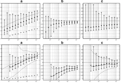
Figure1shows the results for the lognormal distribution with the GP-based esti-mator in the top row, and with the log-GW-based estiesti-mator in the bottom row. The leftmost column (a) shows the medians and the empirical 90 %-intervals (between the 5 % and 95 % percentiles) of the quantile estimates; the width of an empirical 90 %-interval will be referred to as “spread”. The quantilesU (n2)to be estimated are indicated by a dashed curve. Approximate thresholdsU (n/k(n)) andU (n/k0(n))
are indicated by open squares. The middle column (b) shows the parameter esti-matesγˆnm (top) andθˆn (bottom), with the dashed lines indicating the tail indicesγ andθfor the distribution function considered. The rightmost column (c) displays the probability-based errorsνˆnm(top) andνˆn(bottom). For the log-GW-based estimator, also deterministic approximationsq˜yn(2 logn)with withθ˜ =aιandg˜ =gιin (3.1)
and asymptotic 90 % intervals based on (4.18)-(4.20) are displayed. The latter are not confidence intervals, but are shown for comparison against the empirical 5 % and 95 % percentiles and medians of the (biased) estimates in order to verify how good the approximations provided by (4.18)-(4.20) are.
102 103 104 105 100 101 102 103 a 102 103 104 105 −1 −0.8 −0.6 −0.4 −0.2 0 0.2 0.4 0.6 0.8 1 b 102 103 104 105 −1 −0.8 −0.6 −0.4 −0.2 0 0.2 0.4 0.6 0.8 1 c 102 103 104 105 100 101 102 103 a 102 103 104 105 −0.5 0 0.5 1 1.5 b 102 103 104 105 −1 −0.8 −0.6 −0.4 −0.2 0 0.2 0.4 0.6 0.8 1 c
Fig. 1 High quantile estimates for probabilities of exceedance ofn−2on simulated independent standard lognormal samples based on GP (top) and log-GW (bottom) based estimators as functions ofn(see text). Diamonds/vertical bars: median of estimates (black) with 90 % intervals. Left (a): quantile estimates, with target quantilesU (n2)(dashed) and approximate thresholdsU (n/k(n))andU (n/k0(n))(squares). Centre (b): parameter estimatesγˆm
n (top) andθˆn(bottom), dashed lines indicating the indicesγ andθ. Right
(c): errorsνˆm
n (top) andνˆn(bottom). For log-GW only: quantile approximations (-) and asymptotic 90 %
The top row of Fig.1shows the GP-based estimates of logU (n2)apparently set-tling at a fixed distance upward from the exact values, and no convergence ofνˆnm. The parameter estimatesγˆnmappear to converge slowly. In the bottom row, the log-GW-based estimator is seen to perform well, with bias rapidly vanishing. Also, the spreads inqˆnandνˆndrop much more rapidly with increasingnthan forqˆnmandνˆnm.
Figure2for the normal distribution displays a similar pattern as Fig.1, but with some differences. The GP-based estimator now underestimates the very high quan-tiles, even though the parameter estimator γˆm
n converges rapidly. This is the only case in which the sample maximum as lower bound to the quantile estimate became effective. The log-GW-based quantile estimator is performing much better in this case, although convergence is not as rapid as with lognormal data. Based on these results alone, it is not clear whether the bias inνˆnconverges to zero; deterministic computations (not shown) fornup to260with prescribedk2(n)=n1/4show that it vanishes slowly. Forqˆn(2 logn)−q(2 logn), a small nonzero bias eventually remains, but the error relative toq(2 logn)vanishes, and therefore also the error relative to
q(2 logn)−q(yn).
Since the favourable results of the log-GW-based estimator on lognormal data would translate directly to equivalent results with an analogous GW-based estimator on normal data, the latter would do better on the normal data than the log-GW-based quantile estimator in Fig.2. This indicates that in some cases, the speed of convergence may be increased by replacing the latter by a GW-based estimator.
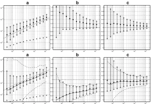
The next two examples concern heavy-tailed distribution functions with classical Pareto tail limitsU ∈ERV(0,∞). By Proposition 1(a), logq∈ERV{1}. Fig.3shows
102 103 104 105 0 1 2 3 4 5 6 7 8 9 a 102 103 104 105 −1 −0.8 −0.6 −0.4 −0.2 0 0.2 0.4 0.6 0.8 1 b 102 103 104 105 −1 −0.8 −0.6 −0.4 −0.2 0 0.2 0.4 0.6 0.8 1 c 102 103 104 105 0 1 2 3 4 5 6 7 8 9 a 102 103 104 105 −1 −0.8 −0.6 −0.4 −0.2 0 0.2 0.4 0.6 0.8 1 b 102 103 104 105 −1 −0.8 −0.6 −0.4 −0.2 0 0.2 0.4 0.6 0.8 1 c
102 103 104 105 100 105 1010 1015 a 102 103 104 105 0 0.2 0.4 0.6 0.8 1 1.2 1.4 1.6 1.8 2 b 102 103 104 105 −1 −0.8 −0.6 −0.4 −0.2 0 0.2 0.4 0.6 0.8 1 c 102 103 104 105 100 105 1010 1015 a 102 103 104 105 0 0.2 0.4 0.6 0.8 1 1.2 1.4 1.6 1.8 2 b 102 103 104 105 −1 −0.8 −0.6 −0.4 −0.2 0 0.2 0.4 0.6 0.8 1 c
Fig. 3 As Fig.1, but for the Pareto-like distribution (U (t)=t (1+2(logt)2)−1) instead of the lognormal
results obtained for the distribution function satisfyingU (t)=t (1+2(logt)2)−1. Concerning bias, both estimators perform rather well as expected. For smalln, the log-GP-based estimator has a much smaller spread than the log-GW estimator; for largen, the spreads are similar. Given that the log-GW based estimator is based on only three order statistics, a large small-sample spread is not surprising. Indeed, replacing the moment estimator by Pickands’ estimator for γ (Pickands (1975)) based on three order statistics, the spread becomes larger than for the log-GW estimator (result not shown).
Finally, Fig.4shows results for the Burr(1,14,4) distribution withU (t)=(t1/4−1)4, which also satisfiesU ∈ ERV{1}. Unlike the previous examples,U has a negative
second-order index (see de Haan and Ferreira (2006)) in this case, so eventually, convergence toward the GP limit should be rapid. As in the previous example, the GP-based estimator performs rather well; the log-GW-GP-based estimator performs similarly but with somewhat larger spread (which is again smaller than obtained when using Pickands’ estimator for the GP-based estimation).
In all figures, the threshold valuesU (n/k0(n))andU (n/k(n))corresponding to the numbersk0(n)andk(n)of upper order statistics used by the estimators are rather different for the two estimators. For the log-GW estimator withι=2,k0(n)must be at leastn3/4irrespective ofk2(n)(see (4.1)), so there is little room for adjustment in order to optimise performance. However, with the GP estimator,k(n)can be reduced considerably to reduce bias if needed. For the lognormal and normal distributions in Fig.1and2, this is seen to lead to a large spread.
102 103 104 105 100 105 1010 1015 a 102 103 104 105 0 0.2 0.4 0.6 0.8 1 1.2 1.4 1.6 1.8 2 b 102 103 104 105 −1 −0.8 −0.6 −0.4 −0.2 0 0.2 0.4 0.6 0.8 1 c 102 103 104 105 100 105 1010 1015 a 102 103 104 105 0 0.2 0.4 0.6 0.8 1 1.2 1.4 1.6 1.8 2 b 102 103 104 105 −1 −0.8 −0.6 −0.4 −0.2 0 0.2 0.4 0.6 0.8 1 c
Fig. 4 As Fig.1, but for the Burr(1,14,4) distribution (see main text) instead of the lognormal
The results tentatively confirm the expectations. For distribution functions in the classical Pareto (γ >0) domain of attraction (satisfying logq ∈ ERV{1}), log-GW
en GP-based estimators seem to perform similarly. However, in the classical domain of attraction of the exponential (γ =0), log-GW may offer advantages.
For the log-GW-based estimator, the asymptotic 90 %-intervals for forθˆn and
ˆ
νnbased on (4.18) and (4.19) provide good approximations to the empirical 90 %-intervals. Forqˆn, the asymptotic 90 % intervals based on (4.20) are in some cases much too wide.
6 Discussion
The log-GW tail limit logq ∈ ERV is a weak assumption of the same nature as the classical regularity assumptionU∈ERV corresponding to the GP tail limit, but specifically aimed toward approximation and estimation of very high quantiles for probabilities in the range (1.5). Proposition 1 indicates that if a GP tail limit applies, then log-GW-based approximation may provide benefits ifγ = 0. Ifγ > 0, then approximation using the GP tail should already be adequate.
Further analysis confirms this: ifU ∈ ERV{0} and logq ∈ ERV, then logq ∈ ERV(−∞,1](see Theorem 2(b)), offering a continuum of tail shapes for
approxima-tion of quantiles where the GP limit withγ = 0 offers only one, the exponential tail.
Suppose thatU ∈ ERV{0}. Then any assumption ensuring convergence of
GP-based quantile approximations with γ = 0 as in (2.8) implies q ∈ RV{1}, so
logq ∈ ERV{0}(1)(see Proposition 1(b)); therefore, it excludes all other
distribu-tion funcdistribu-tions satisfying a log-GW tail limit and a GP tail limit withγ = 0, such as Weibull-like distributions (e.g.the normal distribution), distribution functions of exponents of Weibull-like distributed random variables (e.g.the lognormal distribu-tion), light tails withq(∞)still infinite such asF =1−exp(−exp Id), distribution functions with finiteq(∞)such asF =1−exp((q(∞)−Id)1/θ) withθ <0, just to mention a few which correspond to log-GW or GW limits or are close to such limits. As an example, consider the following seemingly innocent rate assumption for (1.2): lim t→∞ U (tλ)−U (t) w(t) −hγ(λ) logt=0 ∀λ≥1 (6.1) withγ =0. It impliesq∈ERV{1}(see Subsection7.8), and thus by Lemma 1(a) in
Subsection7.9, logq∈ERV{0}(1). Therefore,in the present context, (6.1) is actually
quite restrictive.
The Pareto domain of attraction withγ > 0 is in the domain of attraction of the log-GW tail limit logq ∈ ERV{1} (Proposition 1(a)), so all results obtained for the
latter also apply to the former. Therefore, one might expect that if log-GW based quantile approximation and estimation can not offer improvement ifγ > 0, it may not do much harm either.
This is tentatively confirmed by the results of the simulations in Section5, which indicate that log-GW-based quantile estimation may have merits within theγ = 0 subdomain of attraction of the GP limit and performs similarly to GP-based quan-tile estimation in theγ > 0 subdomain. However, it would be premature to draw conclusions from only these few examples.
For the log-GW based estimatorqˆn, the log-GW limit is sufficient for consis-tency. To establish asymptotic normality, a relatively high rate of convergence (4.21) to the log-GW limit needed to be assumed. As shown in Section4, this is a conse-quence of the particular formulation of this estimator. Therefore, there is a need for alternative estimators which allow the rate condition (4.21) to be relaxed. Based on the simulation results, there appears to be a need for improved accuracy with small sample sizes as well. It is suggested in Section4that bias correction based on esti-mation of a higher-order ERV model could be useful in log-GW-based estimators in order to obtain asymptotic normality while avoiding slow decay of variability with increasingn.
A limitation of log-GW approximation and estimation is that the notions of con-vergence in (3.4) and (4.13) may be weak and cannot be replaced by (3.6) and (4.14) for tails heavier than a typical Weibull tail unless additional assumptions apply. The probability-based errors (3.9) and (4.12) are based on log-ratios of survival func-tions of a quantile and its approximation or estimator. Although natural in view of the probability range considered, a stronger notion of convergence,e.g.of a ratio of survival functions, would be desirable for applications. Stronger notions of conver-gence apply under the additional assumptions for establishing asymptotic normality for the quantile estimatorqˆnin Corollary 1, notably the rate assumption (4.21); see Remark 5.
As a final remark, log-GW-based quantile approximation and estimation for light tails with finite endpoints has only been marginally covered here, so this case remains to be examined in more detail.
7 Proofs and lemmas
7.1 Proof of proposition 1
IfU ∈ ERV{γ}forγ >0, thenU ∈ RV{γ}so by the Potter bounds (e.g.Bingham et al. (1987), Theorem 1.5.6), there is for everyε ∈ (0, γ ∧1)ayε > 0 such that
y(λ−1)(γ−ε)−ε≤logq(yλ)−logq(y)≤y(λ−1)(γ+ε)+εfor ally≥yε and allλ ≥ 1. Therefore, logq ∈ ERV{1}(Id·γ ), so logq ∈ RV{1}. Noting that γ y ∼logq(y)asy → ∞andγ U (t)/w(t) → 1 ast → ∞(both due to de Haan and Ferreira (2006), Theorem B.2.2(1)), we obtain logU˜t(tλ)=logU (t)+log(1+
w(t) γ U (t)(t
(λ−1)γ−1)))=logU (t)+(λ−1)γlogt+o(1)∼λlogU (t)for everyλ≥1, and since logq∈RV{1}, (2.7) follows, so (a) is proven.
Ifγ = 0, (2.8) implies limy→∞(q(yλ)−q(y))/(w(ey)y) = λ−1 ∀λ > 1. Therefore,q ∈ ERV{1}and by Lemma 1(a) in Subsection7.9, logq ∈ ERV{0}(1),
proving (b).
7.2 Proof of theorem 2
Suppose thatU ∈ERV{γ}withγ >0, then as in Subsection7.1, there is for every
ε ∈ (0, γ ∧1) ayε > 0 such that y(λ−1)(γ −ε)−ε ≤ log(q(yλ)/q(y)) ≤
y(λ−1)(γ +ε)+εfor ally ≥ yε and allλ ≥ 1, and therefore, fixingι >1 and
ξ > ι, there is someε∈(0, γ (ξ−ι)/(ξ+ι−2)∧1),δ >0 andzε ≥yεsuch that
q(yξ )−q(y) q(yι)−q(y) ≥
ey(ξ−1)(γ−ε)(1−ε)−1
ey(ι−1)(γ+ε)(1+ε)−1 ≥exp(δy) ∀y≥zε. (7.1) However, sinceq∈ERV, the left-hand side of (7.1) must tend tohθ(ξ )/ hθ(ι) <
∞for some realθasy→ ∞, soγ cannot exceed 0. Assuming thatγ <0, a similar argument leads to a similar contradiction, completing the proof of (a).
For (b), ifU ∈ ERV then by Lemma 1(a) in Subsection7.9, logU ∈ ERV so since logq∈ERV, (a) implies that logU ∈ERV{0}. SinceU ∈ERV and logq∈ ERV, Proposition 1(a) implies that eitherU ∈ ERV(0,∞)and logq ∈ ERV{1}, or U∈ERV(−∞,0]. In the latter case, since logU ∈ERV{0}, Lemma 1(c) implies that U∈ERV{0}⊂RV{0}. Therefore, by the Potter bounds, logq(y)=o(y)asy→ ∞,
so again by the Potter bounds, logqcannot be inRV(1,∞)=ERV(1,∞). 7.3 Proof of proposition 2
Becauseθ (y)˜ →θ andg(y)˜ ∼g(y)asy→ ∞, noting that by (1.4),hθ+o(1)(λ)=
λo(1)hθ(λ), we obtain using the mean value theorem,
locally uniformly inλ > 0. Since (2.9) also holds locally uniformly inλ >0 (see Bingham et al. (1987), Theorem 3.1.16), (3.4) follows from (7.2). If in addition, (3.5) holds, then by (3.4), logq˜y(yλ)−logq(yλ) = (q˜y(yλ)/q(yλ)−1)(1+o(1))as
y → ∞ locally uniformly inλ > 0, and (3.6) follows. Ifq ∈ ERV, then (3.5) follows from Lemma 1(b) in Subsection7.9.
7.4 Clarification of remark 1
Under condition (3.5),q(y)g(y)in (3.6) can be replaced byq(yξ )−q(y)for any
ξ ∈ (0,∞) \ {1}: for ξ > 1, this follows from (3.7), as q(yξ )/q(y) − 1 >
logq(yξ )−logq(y); forξ ∈ (0,1), we findq(yξ )g(y)q(y)−q(y) = q(y)/q(yξ )g(yξ ) −1O(1) =
g(yξ )
logq(y)−logq(yξ )O(1)=O(1)asy→ ∞by regular variation ofgand (3.7). Ifq(∞) <∞, thenq(y)g(y)in (3.6) may be replaced byq(∞)−q(yη)for any
η >0: takingξ >1, q(q(y)g(y)∞)−q(yη) ≤ q(yηξ )q(∞−)g(y)q(yη) ∼ logq(yηξ )g(yη)−logq(yη)g(yη)g(y) =O(1)
asy→ ∞by (3.7) and regular variation ofg. 7.5 Proof of theorem 3
From Proposition 2 and (2.3), asy→ ∞,
logq˜y(yλ)=logq(y)+g(y)(hθ(λ)+o(1)) (7.3) locally uniformly inλ >0. LetΛ >1 andb∈(0, Λ−θ/θ). Applying the mean value theorem tox→h−θ1(hθ(λ)+x)=(λθ+xθ )1/θ, we find that for someM >0,
h−1
θ (hθ(λ)+x)−λ≤Mx ∀λ∈ [Λ−
1
, Λ], x∈ [−b, b].
Therefore, by (7.3), logq˜y(yλ)=logq(y)+g(y)hθ(λ+o(1))uniformly inλ∈
[Λ−1, Λ], so using (2.4),
q−1(q˜y(yλ))= −log
1−Fq(y)eg(y)hθ(λ+o(1))=y(λ+o(1))
uniformly inλ∈ [Λ−1, Λ]. As limz→∞z−1q−1(q(z))=1 by (2.4), we obtain (3.9). 7.6 Proof of theorem 4
Defineˆιm(n)for alln≥1 andm∈ {0,1,2}by
ˆ
ιm(n):=yn−1q−1(Xn−km(n)+1,n)= −y− 1
n log(1−F (Xn−km(n)+1,n)). (7.4)
To simplify notation, we will use
s:=logq, sˆn:=logqˆn, s˜y:=logq˜y. (7.5) Sinceq(∞) > 1, almost surely some n0 ∈ Nexists such that for alln ≥ n0,
(7.26) hold forˆι0(n),ˆι1(n)andˆι2(n)defined by (7.4). Therefore, by (4.3) and (7.25), using (7.5), ˆ θn= 1 logιlog s(ynˆι2(n))−s(ynˆι1(n)) s(ynˆι1(n))−s(ynˆι0(n)) ∀ n≥n0 a.s.
and ass∈ERV{θ}(g)and thereforeg∈RV{θ}, by locally uniform convergence (see Bingham et al. (1987), Theorems 3.1.16 and 1.5.2), and (7.26), almost surely
ˆ θn= 1 logι loghθ(ˆι2(n)/ˆι1(n))+o(1) hθ(ˆι1(n)/ˆι0(n))+o(1)+ logg(ynˆι1(n)) g(ynˆι0(n)) →θ. (7.6) Similarly, using (7.6), almost surely
ˆ gn g(yn) = s(ynˆι1(n))−s(ynˆι0(n)η) g(yn)hθˆn(ι) = hθ(ˆι1(n)/ˆι0(n))+o(1) hθˆ n(ι) g(ynˆι0(n)) g(yn) →1,
so (4.11) is proven. Furthermore, in a similar manner, almost surely
s(yn)−logXn−k0(n)+1,n
g(yn) =
s(yn)−s(ynˆι0(n))
g(yn) = −
hθ(ˆι0(n))+o(1)→0. (7.7) By (4.11), almost surely(gˆn/g(yn))hθˆ
n(λ) →hθ(λ)locally uniformly inλ >0,
so using (7.7),sˆndefined by (7.5) and (4.2) satisfies sup
λ∈[−1,]
sˆn(ynλ)−s(ynλ)/g(yn)→0 a.s. ∀Λ >1. (7.8) Using (4.9), we subsequently obtain (4.13), and (4.14) follows readily as in the proof of Proposition 2. From (7.8) and (2.3), almost surely
ˆ
sn(ynλ)=s(ynλ)+o(g(yn))=s(yn)+g(yn)(hθ(λ)+o(1)) (7.9) locally uniformly inλ >0. By mimicking the proof of Theorem 3 in Subsection7.5
withyn replacingyandsˆn(ynλ)replacings˜y(yλ), we obtain that for everyΛ > 1 almost surely, supλ∈[−1,]νˆn(ynλ)→0; using (4.9), (4.12) follows.
7.7 Proofs of theorem 5 and corollary 1
Using the definitions (7.5), by (4.15), s ∈ RV{θ−1}, so s is a homeomorphism
on some neighbourhood of∞. Therefore, without loss of generality, we can take
sincreasing and continuous, so logXn−km(n)+1,n = s(ynˆιm(n))for allnandm ∈
{0,1,2}. Furthermore, by integration,s∈RV{θ−1}implies
s(yλ)−s(y)=s(y)yhθ(λ)(1+o(1)) (7.10) witho(1)vanishing locally uniformly forλ >0 asy→ ∞9. Therefore, withιˆas in (7.4) and Rm n := logXn−km(n)+1,n−s(ynι m) s(ynιm)ynιm ,
9This implies logU∈ERV
using (7.26) from Lemma 2 in Subsection7.9, almost surely Rm n = s(ynˆιm(n))−s(ynιm) s(ynιm)ynιm ∼ hθ(ι−mˆιm(n))∼ι−mˆιm(n)−1 (7.11) form∈ {0,1,2}. Similarly, forν˜ defined by (3.8) withθ˜ =aι andg˜ =gιin (3.1), substitutingynλ(1+ ˜νyn(ynλ))foryin (7.10) and usings∈RV{θ−1}and Theorems
3 and 4, almost surely,
s(ynλ(1+ ˆνn(ynλ)))−s(ynλ(1+ ˜νyn(ynλ))) s(yn)yn ∼ λθhθ 1+ ˆνn(ynλ) 1+ ˜νyn(ynλ) ∼λθ(νˆn(ynλ)− ˜νyn(ynλ)) (7.12)
locally uniformly forλ >0. From (3.3) and (4.3), using (7.11), (7.10),s∈RV{θ−1}
and (7.26), (θˆn−aι(yn))logι=log ⎛ ⎝1+R2n s(ynι2)ι s(ynι) −R 1 n s(ynι2)−s(ynι) ynιs(ynι) ⎞ ⎠−log ⎛ ⎝1+R1n s(ynι)ι s(yn) −R 0 n s(ynι)−s(yn) yns(yn) ⎞ ⎠ =(hθ(ι))−1 ιθ(ι−2ˆι2(n)−1)(1+o(1))−(ι−1ˆι1(n)−1)(1+o(1)) −ιθ(ι−1ˆι1(n)−1)(1+o(1))+(ˆι0(n)−1)(1+o(1)) a.s. (7.13) Because 1−F (X)has the uniform distribution on(0,1), by Smirnov (1952),
yn(ˆιm(n)−ιm)
km(n) d
→N (0,1) ∀m∈ {0,1,2} (7.14) asn → ∞. Therefore, ask2(n) = o(k1(n))andk1(n) = o(k0(n)), (7.13) implies (4.18). From (4.2) and (3.1), ˆ sn(ynλ)− ˜syn(ynλ) yns(yn) =R 0 n+ haι(yn)(λ) haι(yn)(ι) R1 n s(ynι)ι s(yn) −R 0 n (7.15) + hθˆ n(λ) hθˆ n(ι) −haι(yn)(λ) haι(yn)(ι) s(ynι)−s(yn) yns(yn) +R 1 n s(ynι)ι s(yn) −R 0 n .
Assis increasing and√k2(n)/km(n)log logn→ 0 form∈ {0,1}, Lemma 2(b) in Subsection7.9implies that
(ˆιm(n)−ιm)yn
k2(n)→0 m∈ {0,1} a.s. (7.16) and(ˆι2(n)−ι2)yn√k2(n)=o(log logn)a.s., so by (7.13),(θˆn−aι(yn))yn√k2(n)=
o(log logn)a.s. Therefore, by Taylor’s theorem (see (4.17)), hθˆ n(λ) hθˆ n(ι) −haι(yn)(λ) haι(yn)(ι) −κθ(λ, ι)(θˆn−aι(yn)) =O(1)(θˆn−aι(yn))2 a.s. (7.17) locally uniformly inλ >0, with on the right-hand side (using (4.8)):
By (7.11) and (7.16),Rmnyn√k2(n) → 0 a.s. form ∈ {0,1}. Therefore, from (7.15), using (7.17), (7.18), (7.10) ands∈RV{θ−1}, for all >1,
sup λ∈[−1,] sˆn(ynλ)− ˜syn(ynλ) yns(yn) − κθ(λ, ι)(θˆn−aι(yn))hθ(ι) yn k2(n)→0 a.s. (7.19) Therefore, by (4.18) and (4.9), (4.20) is obtained. Because s is continuously increasing,s(ynλ(1+ ˜νyn(ynλ)))= ˜syn(ynλ)ands(ynλ(1+ ˆνn(ynλ)))= ˆsn(ynλ)in
(7.12) so almost surely,
ˆ
νn(ynλ)− ˜νyn(ynλ)=(1+o(1))λ−
θsˆn(ynλ)− ˜syn(ynλ) yns(yn)
locally uniformly inλ >0. Therefore, using (4.9) and (4.20), we obtain (4.19). This proves Theorem 5.
To prove Corollary 1, note that (4.21) must hold locally uniformly inλ≥1: withr
defined byr(y):=logs(y)−(θ−1)logy, (4.21) is equivalent to limy→∞(r(yλ)− r(y))φ(y)=0 for allλ ≥ 1, which holds locally uniformly inλ ≥ 1 by Theorem 3.1.7c of Bingham et al. (1987). By integration,
s(yλ)−s(y)=ys(y)hθ(λ)(1+o(1)/φ(y)) (7.20) locally uniformly inλ≥1. Therefore,
aι(y)=θ+o(1)/φ(y), (7.21)
so by the mean value theorem,haι(y)(λ)
haι(y)(ι) − hθ(λ)
hθ(ι) =O(aι(y)−θ )=o(1)/φ(y)locally
uniformly inλ≥1. Using (7.20), therefore,
˜ sy(yλ)−s(yλ) ys(y) = s(yι)−s(y) ys(y) hθ(λ) hθ(ι)+
o(1)/φ(y) +s(y)−s(yλ)
ys(y) =o(1)/φ(y)
(7.22) locally uniformly inλ≥1. Finally, by (7.10) and Theorem 3, ass∈RV{θ−1},
s(yλ(1+ ˜νy(yλ)))−s(yλ)∼λθhθ1+ ˜νy(yλ)ys(y)∼λθν˜y(yλ)ys(y) (7.23) locally uniformly inλ ≥ 1. Sincesis continuously increasing,s(z(1+ ˜νy(z))) =
˜
sy(z)for allz >0, so combining (7.23) and (7.22), it follows that
˜
νy(yλ)=o(1)/φ(y) (7.24)
locally uniformly inλ≥1. Usingk2(n)=O(φ2(yn)yn−2), (4.22) follows from (4.18) and (7.21); using (4.9) as well, (4.24) follows from (4.20) and (7.22), and (4.23) follows from (4.19) and (7.24).
7.8 Proof that (6.1) impliesq∈ERV{1}
Takew∈RV{0}. WithRλ(t):=(U (tλ)−U (t))/w(t), (6.1) impliesw(tλ)/w(t)=
(Rλξ(t)−Rλ(t))/Rξ(tλ)=1+o(1/logt)for allλ≥1 andξ >1, so by Bojanic and Seneta (1971) (see Bingham et al. (1987), Theorem 2.3.1),w(tλ)/w(t)→1 locally uniformly inλ ≥ 1 ast → ∞; applying Theorem 3.6.6 in Bingham et al. (1987) givesU (tλ)−U (t)∼(λ−1)w(t)logt for allλ≥1, soq∈ERV{1}.