Journal of Applied Research and Technology 13 (2015) 197-204
1665-6423/All Rights Reserved © 2015 Universidad Nacional Autónoma de México, Centro de Ciencias Aplicadas y Desarrollo Tecnológico. This is an open access item distributed under the Creative Commons CC License BY-NC-ND 4.0.
www.jart.ccadet.unam.mx
Journal of Applied Research
and Technology
* Correponding author.
E-mail address: [email protected] (P. Wang). Abstract
In this paper, we introduce a novel image reconstruction algorithm with Least Squares Support Vector Machines (LS-SVM) and Simulated Annealing Particle Swarm Optimization (APSO), named SAP. This algorithm introduces simulated annealing ideas into Particle Swarm Optimization (PSO), which adopts cooling process functions to replace the inertia weight function and constructs the time variant inertia weight function featured in annealing mechanism. Meanwhile, it employs the APSO procedure to search for the optimized resolution of Electrical Capacitance Tomography (ECT) for image reconstruction. In order to overcome the soft field characteristics of ECT sensitivity field, some image samples with typical flow patterns are chosen for training with LS-SVM. Under the training procedure, the capacitance error caused by the soft field characteristics is predicted, and then is used to construct the fitness function of the particle swarm optimization on basis of the capacitance error. Experimental results demonstrated that the proposed SAP algorithm has a quick convergence rate. Moreover, the proposed SAP outperforms the classic Landweber algorithm and Newton-Raphson algorithm on image reconstruction.
All Rights Reserved © 2015 Universidad Nacional Autónoma de México, Centro de Ciencias Aplicadas y Desarrollo Tecnológico. This is an open access item distributed under the Creative Commons CC License BY-NC-ND 4.0.
Keywords: Electrical capacitance tomography; Simulated annealing algorithm; Least squares support vector machines; Particle swarm optimization
Original
An image reconstruction algorithm for electrical capacitance tomography
based on simulated annealing particle swarm optimization
P. Wang
a,*, J.S. Lin
b, M. Wang
aa School of Electric and Control of Xi’an University of Science and Technology, Xi’an, China
b Department of Computer Science and Information Engineering at National Chin-Yi University of Technology, Taichung, Taiwan Received 19 April 2014; accepted 18 August 2014
1. Introducción
As one of the electrical process tomography imaging tech-nologies, Electrical Capacitance Tomography (ECT) is featured in lower costs, no-irradiative and non-invasive methods, etc., and applicable to the visible measurement of two-phase and multiple-phase flows (York, 2001; Griffiths, 1988). The princi-ple of ECT can be described as: different objects have different permittivities. If the concentration and the composition of the component phase are changed, the permittivity will change to fit the mixture. Variation in permittivity will cause a change of the capacitance measurements and the capacitance measure-ments reflect the size and distribution of the medium phase con-centration of the mixture. On this basis, using a corresponding image reconstruction algorithm can reconstruct the distribution of the test area of the pipeline. Because ECT is non-linearity and the number of capacitances independently measured are
much less than the number of pixels for image reconstruction, there is no resolution for the reverse problem. Furthermore, the sensitivity field of ECT is featured in “soft field”, i.e. sensitivity is not evenly distributed, the reverse problem equation is in a seriously abnormal state (Yang, 1997). Therefore, image recon-struction algorithm has been the bottleneck for the further de-velopment of ECT, and a high precise image reconstruction algorithm is required.
The existing ECT image reconstruction algorithms can be divided into two mainly types: non-iterative algorithm and it-erative algorithm. As one of the typical non-itit-erative algo-rithms, Linear Back Projection (LBP) is simple and quick, but unsatisfying in imaging precision. So LBP is only used as a qualification method (Peng et al., 2004). Iterative methods in-clude: Tikhonov regularization method (Peng et al., 2007), Landweber algorithm (Yang et al., 1999), Newton-Raphson al-gorithm (Yang and Peng, 2003) and Conjugate Gradient meth-od, etc. (Wang et al., 2005). Tikhonov method may cause detailed distortion of the reconstructed images due to over-smoothness of regularization functions. As a widely used meth-od in recent years, Landweber returns satisfying results only
acquisition. Data communication adopts USB2.0 Technology (Yang et al., 2010). As ECT System has more measurement channels, it is difficult for a single DSP to meet real-time re-quirements. Therefore, CPLD or FPGA is generally adopted to conduct auxiliary control of DSP (Ma et al., 2006). ECT image reconstruction unit is composed of two parts: hardware and software. Hardware indicates a general-purpose computer, and software indicates image reconstruction algorithm.
3. ECT image reconstruction
ECT image reconstruction process includes forward and re-verse questions to be resolved. As the forward question, capaci-tance values of all electrode pairs on basis of the permittivity distribution and excitation voltages of the known sensitivity field. The mathematic model of forward question of ECT is ex-pressed as follows (Yang & Peng, 2003):
Ci,j= (x,y)Si,j(x,y)dx dy
(1)where Ci,j is the capacitance between the electrode pair of i-j,
(x,y)is the permittivity distribution on cross-section of pipes,
Si,j(x,y)is the sensitivity functions when the capacitance between
electrode pair of i-j is distributed on the cross-section of pipe,
and is the electrode surface. It can be seen that the sensitivity
of the electrode in a point is related to its position, namely the sensitivity is not evenly distributed within the sensitivity field, which is the so-called effects of “soft field”.
The capacitance sensor comprising of n electrodes can
pro-vide M = n(n – 1)/2 independent capacitances. With M
equa-tions similar with equation (1), such equaequa-tions shall be linearized and discredited to get:
C = S · G (2)
where C is a normalization capacitance vector of M dimension,
G is N dimension normalized permittivity distribution vector,
i.e. the grey level of pixels for visualization, and S is M N
factor matrix, reflects influence of medium distribution varia-with large number of iterations as to complex flow patterns.
Newton-Raphson algorithm is featured in local convergence, but the iterative convergence can’t be guaranteed if the initial value is not selected appropriately. Conjugate gradient method is applicable to positive definite matrix and thus it can’t obtain better effects when it is applied to complex flow patterns.
In this paper, we introduce an image reconstruction algo-rithm with LS-SVM and APSO, which is named as SAP. The proposed SAP is described as follows: firstly, we construct LS-SVM and excise the error between the capacitances arising from sensitivity matrix and the actual capacitance measure-ments; then based on the error, we constructed the fitness func-tion and simulated annealing mechanism for particle swarm optimization; finally, we search for the optimum solution for image reconstruction with APSO.
2. ECT system
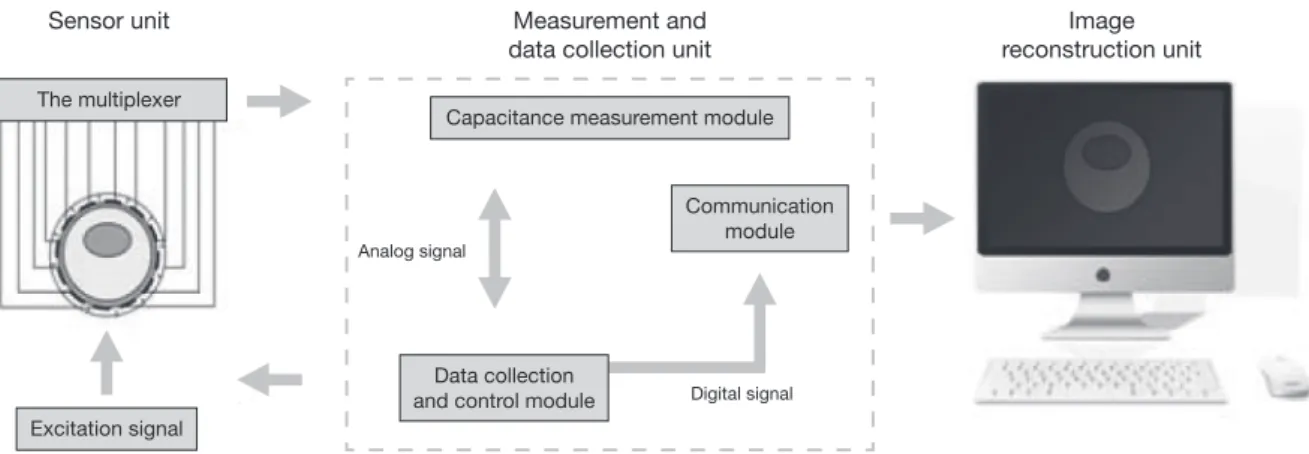
As shown in Figure 1, ECT System is mainly consisted with three units: a capacitance sensor unit, a measurement and data collection unit, and an image reconstruction unit. By utilizing capacitive fringe effect, the sensor can produce a corresponding capacitance for a medium with certain permittivity. The combi-nation of all sensing electrodes may provide multiple capaci-tance measurements, which can be taken as the projection data for image reconstruction. The capacitance measurement and data collection unit primarily functions as rapidly, stably and accurately measuring minor capacitance. It changes in various arrays of electrode couples, and transmits the acquired data to a computer. This unit is mainly comprised of three modules: a capacitance measurement module, a data collection control module, and a communication module. The capacitance mea-surement module is used to realize switching of capacitance to voltage (CV), to measure minor capacitance and effectively in-hibit stray capacitance. Currently, two of the most mature meth-ods to measure capacitance are as follows: capacitance charge-discharge method and AC-based CV switching circuit (Yang, 1996; Yang, 2001) The data collection control module generally takes DSP as the control core and takes ADC for data
Sensor unit Measurement and data collection unit
Image reconstruction unit
Digital signal Analog signal
Capacitance measurement module
Excitation signal The multiplexer
Communication module
Data collection and control module
vid(t+1)= vid(t)+c1r1[Pid(t)xid(t)] +c2r2[Pgd(t)xid(t)]
(5)
xid(t + 1) = xid(t) + vid(t + 1) (6)
Where c1 and c2 are positive constants and called as speedup factors; r1 and r2 are two random numbers between [0,1]; w is called as the inertia factor; i is the ith particle 1 ≤ i ≤ m, d is the dth dimension of each particle 1 ≤ d ≤ D . The initial position and speed of particle swarm is generated randomly, and then iterated according to equations (5) and (6). The position vari-ance range is [xd,min, xd,max] and the speed variance range is [vd,min, vd,max]. The boundary value shall be taken if the dimen-sion of xidor videxceeds the boundary.
4.2. A simulated annealing particle swarm optimization algorithm
The inertia factor in equation (5) keeps particles with the movement inertia of the last generation, and thus particles in-tend to exin-tend the search range. When is larger, the last speed has significant influence and thus has better overall search ca-pabilities; otherwise, the last speed has less influence and thus the local search capability is strong. Local optimization can be skipped by dynamically adjusting . In their studies, Shi and Ebethartln pointed out that the inertia factors reduce gradually with numbers of iteration and thus questions caused by equiva-lent factor are improved (Eberhart & Shi, 1998). In other words, if the resolution after movement of particles are inferior to the solution before movement of particles, the movement shall be accepted at a certain possibility, which shall reduce gradually when time passes. However, the study result of Shi and Ebe-thartln did not definitely give a mathematics definition; they only give a qualitative description with their experiences.
Simulated annealing algorithm is another widely used itera-tive heuristic algorithm. The powerful feature of its intrinsic hill climbing capability (Kirkpatrick, 1983; Sait et al., 2013). On basis of the ideas of Simulated annealing, we introduced a cooling process function (Lin, 2001) to give a quantitative de-scription on the process that the possibility reduces with the reduction of numbers of iteration.
T(t)= 1 +1 +tanh() t T(t1) (7) vid(t+1)=T(t)vid(t)+c1r1
[
Pid(t)xid(t)]
+c2r2Pgd(t)xid(t) (8)4.3. Selection of fitness functions
For each iteration of PSO, the fitness function is used to de-termine whether the position of particle is satisfied or dissatis-fied. When PSO is applied to the image reconstruction of ECT, the fitness function is generally taken as follows:
F = min (C – S · G) (9) tion on capacitance C, and is called as sensitivity matrix
(Tik-honov & Arsenin, 1977).
Si,j()=Ci,j()C l i,j Ch i,jC l i,j (3)
Where Si,j() is the th unit of electrod pair to i-j sensitivity matrix, Ci,j() is the measurement capacitance, Ci,j(l) is the ca-pacitances when the sensor is full of lower permittivity medi-ums, and Ci,j(h) is the capacitances when the sensor is full of higher permittivity mediums.
The reverse question is to reconstruct permittivity distribu-tion diagram in the sensitivity field with capacitance measure-ments and sensitivity matrix S representing grey levels of pixels. Currently, most of the image reconstruction algorithms are achieved with the basis of:
G = S–1C (4)
There is no annalitic resolution for equation (4). Firstly, per-mittivity distribution is not linear with the capacitance mea-surements at boundaries in sensitivity field. Secondly, the data M is independently measurements and far less than the number of pixels N, therefore the solution of equation (4) is not unique. Furthermore, the equation (4) is ill posed, and the resolution is not stable. Minor error of C may have significant influences on G (Yeung & Ibrahim, 2003.). In addition, the matrix S is not truly constant, but varies with the actual permittivity distribu-tion. Therefore, we try to resolve reverse question of ECT with a heuristic algorithm to achieve high-precise imaging in this paper.
4. Image reconstruction algorithm on basis of simulated annealing particle swarm optimization
4.1. Conventional particle swarm optimization algorithm Particle swarm optimization (PSO) is a well known heuristic algorithm, which is firstly proposed by Kennedy and Eberhart (1995) and is sourced from studies on food-catching of birds. Many kinds of PSO algorithms have been widely studied and have made certain achievements in the last twenty years (Reza-zadeh et al., 2009; Arce et al., 2012; Gerardo et al., 2009). In PSO system, each alternative resolution is called as a “particle”. Particles are co-existing and shall be optimized. That is be-cause each particle should “fly” towards to a better position in the question space according its own experiences to explore the best resolution. The mathematic expression of PSO is shown as follows (Eberhart & Shi, 2000).
In this paper, we presume the space is D-dimension and the scale of particles are m. The position of the ith particle is Xi = (xi1, xi2,…, xiD) . The best position of the ith particle in the “fly-ing” history is Pi = (pi1, pi2,…, piD), and we presume the best value of Pi(i = 1,2,…,m) is located at Pg; the velocity of the ith particle is the vector of V
i = (vi1, vi2,…, viD); the position of ith particle will change according to the following equations:
According to the optimization conditions, we make the par-tial derivative of L against w, b, e and as zero, and eliminate variant w and e and thus get the following linear equation:
0 T +1 b = 0y (15)
Where, y = [y1, y2,…, y], = [1, 2,…, ] and is column vectors with k dimension as 1 and ij=( )xi
T
( )
xj .Accord-ing to the principle of Mercer, the mappAccord-ing function () and kernel function () existing and thus:
K
(
xi,xj)
=( )
xi T( )
xj i,j=1,2,..., (16)The function estimates expression of the least square algo-rithm is as follows:
f( )x = i i=1
K
( )
x,xi +b (17)Where, i(i = 1,2,…,) and b are obtained from equation (15), the specific forms of f(x) is subject to types of function K(x,xi). There are many kinds of kernel functions. In this pa-per, we take the kernel function of radial basis (i.e. Gaussian) with higher regression capabilities which is defined as fol-lows: K
( )
x,xi =exp xxi 2 2 (18)Where, is Gaussian kernel parameter.
5.2. Functions of LS-SVM in ECT image reconstruction As described above, due to the soft field characteristics of ECT, the capacitance calculated through equation (2) and the actual measurement of capacitance have the following e rrors:
C=CSG (19)
where, G– is actual permittivity distribution vector. In order to get the capacitance error C under any permittivity distribu-tion, we take use of LS-SVM to exercise certain of quantities of samples with LS-SVM. Taking samples of vectors into equa-tion (19) and get:
y= C = CSG = f x( ):Rn
R1 (20)
where the input vector x is normalization capacitance vector, and the output y is the norm of samples of capacitance error. When carrying out exercises with LS-SVM, the input sample collection is actual capacitance vector under all kinds of flow patterns, and output sample collection is the norm of samples of capacitance error under all kinds of flow patterns.
Where C is the normalization measurement capacitance vec-tor, S is a sensitivity matrix and G is position vector of particle (i.e. the required permittivity distribution vector).
Due to the matrix S is not truly constant, but varies with the actual permittivity distribution. PSO taking takes equation (9) as the fitness function, which can achieve an overall optimiza-tion of convergence and there may be larger error between the optimization resolution and actual distribution of permittivity. The fitness function in this paper is given as the following:
F = min(C – S · G –C) (10) Where C is the output when LS-SVM takes C as input. The fitness function takes use of the results predicted by LS-SVM so as to eliminate errors arising from that different flow patterns under the same sensitivity matrix S.
5. Least squares support vector machine and its applications in image reconstruction
5.1. Least squares support vector machine
LS-SVM is a kernel function study machine complying with Structural Risk Minimization (SRM) algorithm of the least square algorithm and principle of SRM (Gu et al., 2010). The concept is described as follows: specify sample collection {xi,yi}
i=1 map n-dimension input vector Xi and output vector Yi from the original space Rn to the high dimension special space Rn+ through non-linear transformation (x).In this space the opti-mization linear decision function is given as the following:
f(x) = w · (x) + b (11) Where, W is a hyper plane weight vector, and b is a polarization item. For LS-SVM, the question to be optimized is as follows:
min
(
w,e)
=1 2w T w+1 2 ei 2 i=1 (12)Where, ei is an error variant; > 0 is a punitive parameter controlling the punishment for samples exceeding errors. LS-SVM converts the inequality constraints into equality con-straints (Ott et al., 1990). For LS-SVM for regression estimate, the constraints are as follows:
yi=w T
( )
xi +b+ei, i=1,2,..., (13)According to KKT conditions, the Lagrange factor iR (i.e. support vector factor) is introduced to construct Lagrange function. L
(
w,b,e,)
=1 2w T w+1 2 ei 2 i=1 i w T( )
xi +b+eiyi(
)
i=1 (14)The experimental results of the relative image error are shown in Table 2. From Table 2 we can see that the quality of reconstruction image with SAP for all above flow types are sig-nificantly improved by comparing with Newton-Raphson and Landweber algorithms.
The elapsed time required for reconstruction of the three different algorithms are shown in Table 3. Obviously, the number of iterations for landweber and Newton-Raphson al-gorithms are greater than that for SAP algorithm. It is inter-esting to see from Table 3 that, in four cases, the elapsed time for the SAP algorithm is less larger than that for the Landwe-ber algorithm, and is shorter than that for the Newton-Raph-son algorithm.
7. Discussion on chaos search
The chaotic movement is a kind of non-periodic bounded dynamic activity sensitive to initial conditions in definite sys-tems. The chaotic movement is featured in false randomness, ergodicity and sensitivity to boundaries, etc. (Liu et al., 2006). Chaotic theory has been widely used in particle swarm Optimi-zation algorithm (Alatas et al., 2009). When it is determined that PSO algorithm is under premature convergence conditions, the diversity of groups and sustaining searching capabilities of particles can be improved with the chaotic search.
7.1. Chaotic annealing particle swarm optimization
Many rules can cause chaos and the representative chaotic model is Logistic equation (Chen & Zhao, 2009).
6. Simulation results and analysis
6.1. Algorithm flow process
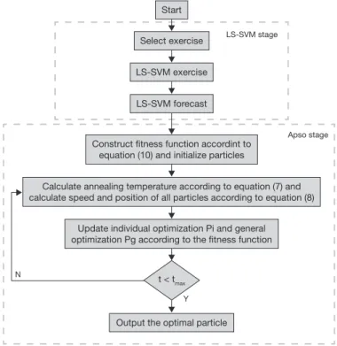
The SAP algorithm comprises of LS-SVM exercise forecast stage and APSO search stage. The algorithm flow process is shown as Figure 2, in which t is current iteration times of APSO.
In LS-SVM stage, 40 groups of samples including 4 kinds of flow patterns are used as exercise samples, the punitive param-eter and the kernel parameter shall be selected through ex-periences. Based on the exercise results of LS-SVM, forecast of the test samples and capacitance error C are achieved. In this paper, we select 8 electrode capacitance sensors to get 28 separated capacitance measurements and thus the input sam-ple data of LS-SVM xi is 28-dimension (i = 1,2,…,40). Capaci-tance measurements can be obtained with finite element methods. In finite subdivision, we take triangle unit to subdi-vide the imaging area into 800 units, and we take finite subdivi-sion unit as the pixel unit of images and the permittivity distribution G– under all kinds of flow patterns of sample is an 800-dimension vector.
In APSO stage, we firstly construct fitness function according to equation (10), then initialize particle swarm. The swarm scale is set as m=40, the number of dimensions is same as the number of pixels in image domain, i.e. D = 800. The maximum iteration number is tmax. We set up limit position of particles and variance range between limit speed and particle speed. Finally, we search for the optimum solution for image reconstruction with APSO. 6.2. Experimental results and evaluation on algorithm
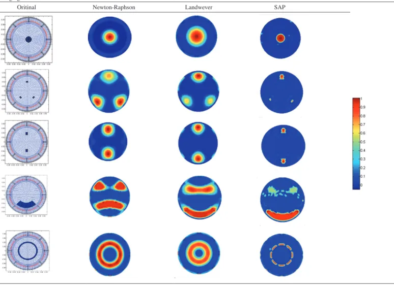
In order to validate effectiveness of the algorithm, we take SAP algorithm to make image reconstruction for typical flow patterns (i.e. core flow, bubble flow, laminar flow, and circular flow), and then compared them with the imaging results of Newton-Raphson algorithm and Landweber algorithm. The simulation and calculation is carried out with MATIAB 7.10 on Intel Pentium 820 MHz CPU (RAM 512 MB). The experimen-talresults are shown in Table 1. In imaging area, the dark area is even medium of permittivity 40 and the other areas is air (i.e. permittivity 1.0).
As shown in Table 1, we can see that imaging results with Landweber algorithm and Newton-Raphson algorithm are near to the original; however, there are too many false images. Obvi-ously, the quality of images obtained with SAP is much better, for which the resolution of images is much higher and there is nearly no false image.
When the quality of image is analyzed, the relative image error shall be used as evaluation index of image quality, which is defined as follows:
image=
gg
g (21)
where, g^ is permittivity distribution vector obtained with recon-struction algorithm, and g is permittivity distribution vector in the original. ·is a vector sample norm, which here is taken as 2.
Start
Select exercise
LS-SVM exercise
LS-SVM forecast
Output the optimal particle Construct fitness function accordint to
equation (10) and initialize particles
Calculate annealing temperature according to equation (7) and calculate speed and position of all particles according to equation (8)
Update individual optimization Pi and general optimization Pg according to the fitness function
LS-SVM stage
Apso stage
N
Y
t < tmax
zdk+1=uz d k
(1Zdk
) k=0,1,2,...kmax (22) where u is absorption factor, k is iteration times, and d is di-mensions in question. When u = 4,zd0 (0,1), the equation (22) will be completely under chaos conditions and zdk + 1 shall tour through (0,1) along with the iteration process.
Application of the chaotic search in SAP algorithm is repre-sented in the following two procedures:
1. Initialization of algorithm: generally, the scale of cha-otic group mCHOAS is 0.3 times of the original group scale. We need set up the maximum iterations kmax and give initial values to zdk with minor differences separate-ly and then get d chaotic variables zdk with different tracks.
2. Searching with chaotic variables: the chaotic variables are mapped from chaotic space to the solution space for optimization of questions and chaotic search. After each step of iteration, a solution may be created for the solu-tion space.
With kmax iteration, the solution mapped from chaotic vari-ables will tour through the solution space for optimization ques-tions and thus make full optimization.
Table 1 Imaging result.
Oritinal Newton-Raphson Landwever SAP
Table 2
Relative image error.
Original Newton-Raphson Landweber SAP
1 33% 41.8% 16.0% 2 37.6% 40.2% 19.5% 3 42% 40% 21% 4 71% 65% 41% 5 32.8% 40.1% 24% Table 3
Elapsed time (in seconds).
Original Newton-Raphson Landweber SAP
1 10.77s 500 iterations 3.61s 100 iterations 5.09s 80 iterations 2 11.12s 500 iterations 4.98s 130 iterations 9.10s 120 iterations 3 10.90s 500 iterations 5.04s 130 iterations 9.24s 120 iterations 4 14.05s 800 iterations 7.28s 200 iterations 12.55s 150 iterations 5 12.18 600 iterations 33.7s 5000 iterations 16.08s 180 iterations
where l is the length of diagonals of the search space, m is group scale, D is the dimension of solution space, xid is dth dimension coordinates of ith particle, and x—d is the average value of xid.
2= 1 m fi favg f i=1 m
2f = max1im fifavg max1im fifavg >1
1 other (26)
where fi is the value of fitness function of ith particle, favg is av-erage value of fitness functions of all particles. When 2 or D(t) is less than the given thresholds, it may be considered that the algorithm has been under premature convergence conditions. 7.2. Performance analysis of CAPSO algorithm
In order to analyse the performance of chaotic search in SAP algorithm, we take SAP algorithm to make image reconstruc-tion for typical flow patterns (core flow, bubble flow, laminar flow and circular flow), and then compared them with the imag-ing results of CAPSO algorithm. The imagimag-ing results are shown in Table 4. From Table 4, we can see that imaging results of the two kinds of algorithms are almost the same. It indicates that SAP algorithm embedding chaotic search did not significantly improve the imaging precision.
The mapping relationship between the variable xd [xd,min, xd,max] and chaotic variable zd [zd,min, zd,max] shall be specified by equation (23) and (24) (Krilc et al., 2002).
xd =xd,min+(
zdzd,min)(xd,maxxd,min)
zd,maxzd,min (23)
zd=zd,min+(
xdxd,min)(zd,maxzd,min)
xd,maxxd,min (24)
The chaotic search is carried out when the particle swarm algorithm is under premature convergence conditions, i.e. mak-ing secondary search in small field neighbormak-ing local optimal values so as to get away from local optimal values. Premature convergence is used to search for the overall optimal values with particles. All particles are trending to be collected to the same extreme point, thus the diversity of particles is gradually decreased. If such extreme value is locally optimal one, the al-gorithm is under premature convergence conditions. In this pa-per, we take the average particle distance D(t) and the fitness value variance 2 (Lv & Hou, 2004) as the conditions for deter-mination of premature convergence.
D(t)= 1 lm (xidxd) 2 d=1 D
i=1 m (25) Table 4Imaging results of SAP and CAPS.
Eberhart, R., & Shi, Y. (2000). Comparing inertia weights and constriction factors in Particle Swarm Optimization. Proceedings of the Congress on Evolutionary Computation, 1, 84-88.
Griffiths, H. (1988). A phantom for electrical impedance tomography.
Clinicalphysics and Physiological Measurement, 9, 15-20.
Gerardo, A., Mauricio, O.C., Nareli, C.C, Ricardo, B.F., & Jessus, A.A.C. (2009). Comparative study of parallel variants for a particle swarm optimization algorithm implemented on a multithreading GPU. Journal of Applied Research and Technology, 7, 292-309.
Gu, Y.P., Zhao, W.J., & Wu Z.S. (2010). Least squares vector machine algorithm. Journal of Tsinghua University (Science & Technology), 50,
1063-1066.
Kirkpatrick, S. (1983). Optimization by simulated annealing: quantitative studies. Journal of Statistical Physics. 34, 975-986.
Krilc, T., Vesterstrom, J.S., & Riget, J. (2002). Particle swarm optimization with spatial particle extension. Proceedings of the World on Congress on Computational Intelligence, 1474-1479.
Lv, Z.X., & Hou, Z.R. (2004). Particle swarm optimization with adaptive mutation. Acta Electronic Sinica, 32, 416-420.
Lin, J.S. (2001). Annealed chaotic neural network with nonlinear self-feedbackand its application to clustering problem. Pattern Recognition, 34, 1093-1104.
Liu, H.B., Wang, X.H., & Tan, G. (2006). Convergence analysis of particle swarm optimization and its improved algorithm based on chaos. Control and Decision, 21, 636-645.
Ma, M., Wang, H.X., & Tian, L.M. (2006). Electrical capacitance tomography system based on DSP. Chinese Journal of Sensors and Actuators, 19,
705-708.
Ott, E., Grebogi, C., & Yoke, J.A. (1990). Controlling chaos. Physical Review Letters. 64, 1196-1199.
Peng, L.H., Lu, D., & Yang, W.Q. (2004). Image reconstruction algorithms for electrical capacitance tomography: state of the art. Journal of Tsinghua University (Science & Technology), 44, 478-484.
Peng, L.H., Jiang, P., Lu, G., & Xiao, D. (2007). Window function-based regularization for electrical capacitance tomography image reconstruction. Flow Meas Instrum, 18, 277-284.
Rezazadeh, H., Ghazanfri, M., & Sadjadi, S.J. (2009). Linear programming embedded particle swarm optimization for solving an extended model of dynamic virtual cellular manufacturing systems. Journal of Applied Research and Technology. 7, 83-108.
Sait, S.M., Sheikh, A.T., & ElMaleh, A.H. (2013). Cell assignment in hybrid CMOS/Nanodevices architecture using a PSO/SA hybrid algorithm.
Applied Research and Technology, 11, 653-664.
Tikhonov, A.N., & Arsenin, V.Y. (1977). Solutions of ill-posed problems (1st ed.). Washington, DC: Winston.
Wang, H.X., Zhu, X.M., & Zhang, L.F. (2005). Conjugate gradient algorithm for electrical capacitance tomography. Tianjin University, 38, 1-4. York, T. (2001). Status of electrical tomography in industrial applications.
Electronic Imaging, 10, 600-619.
Yang, W.Q. (1997). Modeling of capacitance tomography sensors. IEE Proceedings: Science, Measurement and Technology. 114, 203-208. Yang, W.Q., Spink, D.M., York, T.A., & McCann, H. (1999). An
image-reconstruction algorithm based on Landweber’s iteration method for electrical capacitance tomography. Measurement Science and Technology, 10, 1065-1069.
Yang, W.Q., & Peng, L.H. (2003). Image reconstruction algorithms for electr ical capacita nce tomography. Measurement Science and Technology, 14, R1-R13.
Yang, W.Q. (1996). Hardware design of electrical capacitance tomography systems. Measurement Science and Technology, 7, 225-232.
Yang, W.Q. (2001). Further developments in an ac-based capacitance tomography system. Review of Scientific Instruments, 72, 3902-3907. Yang. D.Y., Xu, C.L., & Zhou, B. (2010). Electrical capacitance tomography
system based on single measurement channel. Chinese Journal of Scientific Instrument, 31, 132-136.
Yeung, H., & Ibrahim, A. (2003). Multiphase flows sensor response database.
Flow Measurement and Instrumentation, 14, 219-223. In the worst case, the time complexity of the SAP and CAPSO
algorithms are O(tmaxm2D) and O(tmaxm2DmchaoskmaxD), where, m is group scale, D is the dimension of particles, tmax is the max iterations, mchaos is the chaotic group scale, and kmax is the maximum chaotic iterations.
Obviously, the time complexity of the CAPSO algorithm is much greater than that of the SAP algorithm.
8. Conclusions
In this paper, we have introduced an ECT image recon-struction algorithm on basis of LS-SVM and APSO, named SAP algorithm. In order to propose this algorithm, we intro-duced annealing ideas into particle swarm optimization algo-rithm, taking cooling process function to replace inertia factor and constructing the time variant inertia weight function fea-tured in annealing mechanism. As errors caused by the fixed sensitivity matrix for ECT reverse questions, we took LS-SVM to exercise for the errors and apply exercise results to the improvement of APSO. Then the optimized resolution of reconstructed images was searched. The experimental re-sults demonstrated that using SAP algorithm can get high pre-cise reconstructed images.
Finally, in order to further improved the precision of SAP algorithm, chaotic search process was merged into SAP. Ex-perimental results demonstrated that though SAP algorithm embedding chaotic search did not significantly improve the im-aging precision. However the time complexity of the algorithm is greatly improved.
Acknowledgements
This work is financially supported by Projects 51405381 and 51475013 from the National Natural Science Foundation of China, Project 201314 supported by Engagement Foundation of Xi’an University of Science and Technology, and a Project sup-ported by Scientific Research Foundation for Returned Schol-ars, Ministry of Education of China 2011508
References
Arce, A., Covarrubias, D.H., Panduro, M.A., & Garza, L.A. (2012). Design of beam-forming networks for multibeam antenna arrays using coherently radiating periodic structures. In Proceedings of International Congress on 1st Instrumentation and Human Applied Science, 10, 48-56. Alatas, B., Akin, E., & Ozer, A.B. (2009). Chaos embedded particle swarm
Optimization algorithms. Chaos Solutions & Fractals, 40, 1715-1734. Chen, C., & Zhao, C.X. (2009). Path test data generation based on chaos
anneal particle swarm optimization. Journal of Nanjing University of Science and Technology, 3, 376-381.
Eberhart, R., & Kennedy, J. (1995). A new optimizer using particles swarm theory. In Proceedings of the Sixth International Symposium on Micro Machine and Human Science, 7, 39-43.
Eberhart, R., & Shi, Y. (1998). Parameter selection in particle swarm optimization. Proceedings of Evolutionary Programming, 1447, 591-600.