2012
Borrowing information across genes and
experiments for improved error variance estimation
in microarray data analysis and statistical inferences
for gene expression heterosis
Tieming Ji
Iowa State University
Follow this and additional works at:
https://lib.dr.iastate.edu/etd
Part of the
Biostatistics Commons
This Dissertation is brought to you for free and open access by the Iowa State University Capstones, Theses and Dissertations at Iowa State University Digital Repository. It has been accepted for inclusion in Graduate Theses and Dissertations by an authorized administrator of Iowa State University Digital Repository. For more information, please [email protected].
Recommended Citation
Ji, Tieming, "Borrowing information across genes and experiments for improved error variance estimation in microarray data analysis and statistical inferences for gene expression heterosis" (2012).Graduate Theses and Dissertations. 12761.
estimation in microarray data analysis and statistical inferences for gene expression heterosis
by
Tieming Ji
A dissertation submitted to the graduate faculty in partial fulfillment of the requirements for the degree of
DOCTOR OF PHILOSOPHY
Co-majors: Bioinformatics and Computational Biology; Statistics
Program of Study Committee: Dan Nettleton, Co-major Professor
Peng Liu, Co-major Professor Patrick Schnable, Co-major Professor
Dan Nordman Huaiqing Wu
Iowa State University Ames, Iowa
2012
DEDICATION
TABLE OF CONTENTS
LIST OF TABLES . . . vi
LIST OF FIGURES . . . vii
ACKNOWLEDGEMENTS . . . x
ABSTRACT . . . xi
CHAPTER 1. GENERAL INTRODUCTION . . . 1
1.1 Introduction . . . 1
1.2 Gene Expression and Microarray Technology . . . 1
1.3 Shrinkage Method for Error Variance Estimation . . . 2
1.4 Heterosis and Gene Expression Heterosis . . . 4
1.5 Estimation and Testing of Gene Expression Heterosis . . . 5
1.6 Dissertation Organization . . . 5
Bibliography . . . 6
CHAPTER 2. BORROWING INFORMATION ACROSS GENES AND EXPERIMENTS FOR IMPROVED ERROR VARIANCE ESTIMATION IN MICROARRAY DATA ANALYSIS . . . 9
2.1 Introduction . . . 10
2.2 Standard Linear Modeling of Expression Data and Tests of Interest . . . 12
2.3 A Proposed Model for Error Variances and the Resulting Bayes Estimates . . . 13
2.4 Permutation Test . . . 16
2.5 Simulation Studies Based on Probability Models . . . 18
2.5.2 Simulated Cases with Different Degrees of Freedom across Experiments 23
2.6 Real Data Simulation Examples . . . 24
2.7 Analysis of the Study on Aerenchyma Formation in Maize Roots . . . 26
2.8 Conclusions and Discussion . . . 27
2.9 Appendix . . . 28
2.9.1 Treatments in the Motivating Experiments . . . 28
2.9.2 Parameter Estimation . . . 30
2.9.3 Computation ofΣ−1 . . . 31
2.9.4 Computation of(Σ−1+V−1)−1 . . . 32
2.9.5 Generating Microarray Expression Data with Treatment Effects . . . 32
2.9.6 Generating Error Variances Following Inverse Gamma Priors for Multiple Microarray Experiments . . . 33
2.9.7 Results and Discussion When Changing Hyperparameter Values . . . 34
2.9.8 Complementary Contour Plots . . . 36
Bibliography . . . 37
CHAPTER 3. ESTIMATION AND TESTING OF GENE EXPRESSION HETEROSIS . . . 40
3.1 Introduction . . . 41
3.2 Hierarchical Model for Gene Expression Heterosis . . . 43
3.3 Empirical Bayes Estimation and Testing of Gene Expression Heterosis . . . 45
3.4 Example Data Analysis . . . 49
3.4.1 Analysis of an Alfalfa Dataset . . . 49
3.4.2 Analysis of a Maize Dataset . . . 52
3.5 Simulation Studies . . . 53
3.5.1 Simulation Descriptions . . . 53
3.5.2 Simulation Study based on the Alfalfa Experiment . . . 53
3.5.3 Simulation Study based on the Maize Experiment . . . 56
3.5.4 Simulation Study based on Probability Models . . . 58
3.7 Appendix . . . 61
3.7.1 Appendix A: Problems of Sample Average Method in Estimatinghj’s and lj’s . . . 61
3.7.2 Appendix B: Derivation and Approximation of the Joint Posterior Distri-bution ofαj and δj . . . 63
3.7.3 Appendix C: Estimation of Hyperparameters . . . 67
Bibliography . . . 69
CHAPTER 4. STATISTICAL ANALYSIS FOR THE STUDY OF POTEN-TIAL CARBON CAPTURING CROPS . . . 72
4.1 Introduction . . . 73
4.2 Experimental Design and Data Collection . . . 74
4.3 Statistical Modeling and Estimation of Carbon Dioxide Emission . . . 75
4.4 Analysis of the Association of Lignin Content with CO2 Emission . . . 82
4.5 Conclusions and Discussion . . . 83
4.6 Appendix . . . 87
4.6.1 Appendix A: Observation Days and Placement of Samples. . . 87
4.6.2 Appendix B: Fitting Results for Genotype Effect . . . 87
4.6.3 Appendix C: Extrapolation of Nighttime Soil Temperatures . . . 89
Bibliography . . . 92
LIST OF TABLES
Table 2.1 Comparison of bias, mean square error, area under ROC curves, false
positive number (V), positive number (R), and V/R for simulations
5.1-5.4 and 6.1-6.2. . . 21
Table 2.2 Number of reported positives for each experiment in the four motivating
experiments by three different methods. . . 27
Table 2.3 Comparisons in the four motivating experiments. . . 29
Table 2.4 Selected slides for analysis in the paper. . . 29
Table 2.5 Parameter values for generating treatment effect for simulations 5.1 –
5.4 and 6.1 – 6.2. . . 33
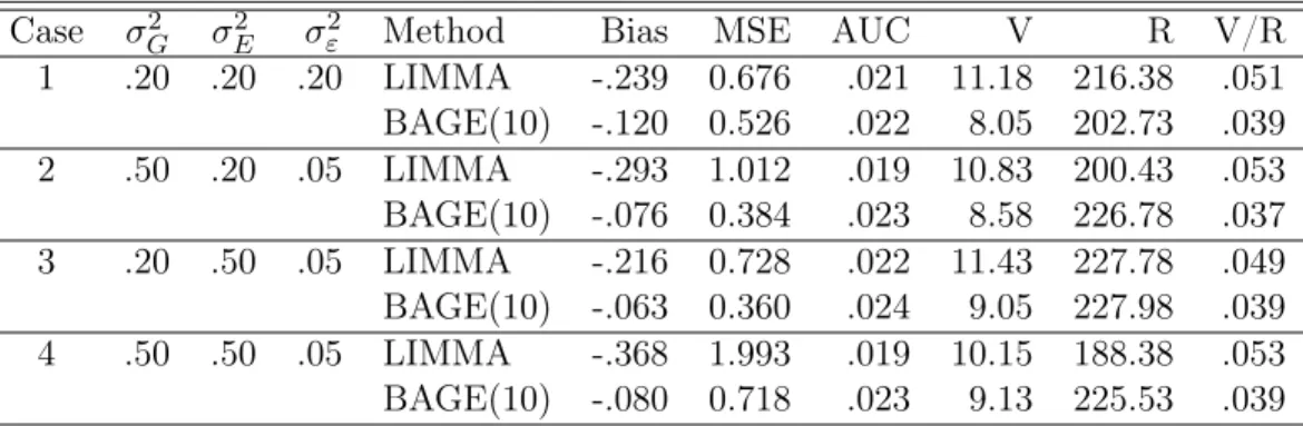
Table 2.6 Parameter values and simulation results for four different cases. . . 35
Table 3.1 Estimated hyperparameters (obtained by using the methods described in
Appendix C) and the bias and MSE estimates (obtained by parametric
bootstrap) for the alfalfa and maize experiments. . . 49
Table 3.2 Number of genes declared to exhibit gene expression heterosis by the
sample average method and the empirical Bayes method. . . 52
Table 3.3 Comparison of bias and MSE of the empirical Bayes estimates and the
sample average estimates. . . 56
Table 4.1 Estimated accumulated flux (mol/m2) for two stages and the entire 164
days. . . 80
Table 4.2 Arrangement of 60 samples on 6 shelf levels with 10 positions on each
shelf. . . 87
LIST OF FIGURES
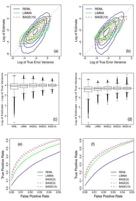
Figure 2.1 Comparison of REML, LIMMA, and BAGE methods. Left column: data
are simulated under the lognormal model (simulation 5.1). Right col-umn: data are simulated under the inverse gamma model (simulation 5.2). Top row: contour plots to compare estimates of error variances. Middle row: box plots of estimation errors in log scale. Bottom row:
ROC curves. . . 20
Figure 2.2 Comparison of the ordinaryt-test based on REML estimates, the
mod-erated t-test based on LIMMA estimates and the FBAGE test based on
BAGE estimates through simulations based on real data sets. (a) True error variances are simulated based on the ALL data set (simulation 6.1). (b) True error variances are simulated based on the Golub data set
(simulation 6.2). . . 26
Figure 2.3 Contour plots of simulations 5.1 – 5.4. (a) Simulation 5.1. Equal degrees
of freedom across experiments with true error variances sampled from the lognormal model. (b) Simulation 5.2. Equal degrees of freedom across experiments with true error variances sampled from the inverse gamma model. (c) Simulation 5.3. Different degrees of freedom across experiments with true error variances sampled from the lognormal model. (d) Simulation 5.4. Different degrees of freedom across experiments with
Figure 3.1 Scatter plots of αbj’s and bδj’s based on two real heterosis experiments.
(a) Alfalfa dataset. B2, B5 and F1 denote the genotypes of the two parental inbred lines and the hybrid offspring, respectively. (b) Maize dataset. B73, Mo17 and F1 denote the genotypes of the two parental
inbred lines and the hybrid offspring, respectively. . . 44
Figure 3.2 Example HPH gene (gene number 40 in the alfalfa dataset). . . 50
Figure 3.3 Segmentation of scatter plots of αbj’s andδbj’s based on analysis results.
By the empirical Bayes method, genes are declared of exhibiting HPH (red), LPH (blue), MPH but not HPH or LPH (green) are plotted, as well as genes not tested to exhibit any form of gene expression heterosis
(black). . . 51
Figure 3.4 Plots for the simulation study based on the alfalfa experiment data. Top
row: box plots of ranked estimation errors averaged over 100 simulations. Middle row: ROC curves averaged over 100 simulations. Bottom row: estimated FDRs based on posterior probabilities versus true FDRs. Left
column: HPH. Middle column: LPH. Right column: MPH. . . 55
Figure 3.5 Plots for the simulation study based on the maize experiment data. Top
row: box plots of ranked estimation errors averaged over 100 simulations. Middle row: ROC curves averaged over 100 simulations. Bottom row: estimated FDRs based on posterior probabilities versus true FDRs. Left
column: HPH. Middle column: LPH. Right column: MPH. . . 57
Figure 3.6 Plots for the simulation study based on hypothetical probability models
that violate the model assumptions of the empirical Bayes method. Top row: box plots of ranked estimation errors averaged over 100 simulations. Middle row: ROC curves averaged over 100 simulations. Bottom row: estimated FDRs based on posterior probabilities versus true FDRs. Left
Figure 4.1 Estimated CO2flux from crop residue decomposition across 14 genotypes
and 164 days. . . 78
Figure 4.2 Estimated accumulated CO2 flux from crop residue decomposition for
each genotype for the first 10 days and last 155 days. . . 79
Figure 4.3 Correlation of estimated CO2 flux and lignin content. (a) Correlation
of estimated total CO2 flux from day 1 to day 10 and lignin content.
(b) Correlation of estimated total CO2 flux from day 10 to day 164 and
lignin content. (c) Correlation of estimated total CO2 flux of the entire
164 days and lignin content. . . 84
Figure 4.4 Correlations of lignin content and accumulated flux of two stages when
choosing different days to define the break point between stage 1 and
stage 2. . . 85
Figure 4.5 Room temperature and soil temperature measurements over 164 days.
The black points are for room temperatures measured by machines in the greenhouse, and the green points are for soil temperatures measured
by researchers. . . 90
Figure 4.6 Temperatures of 24 hours across 164 days. . . 90
Figure 4.7 Scatter plot of the daytime room temperatures and soil temperatures
ACKNOWLEDGEMENTS
I would like to take this opportunity to express my many thanks to those who helped me with various aspects in graduate studies and research. Firstly, I feel very grateful for having the opportunity to start my Ph.D. study at the Iowa State University about five years ago, where the research in both statistics and biology is nationally renowned. I have taken several classes both in the BCB program and the Statistics Department. In consulting and collaborative work as well as summer intern work, I was able to make a contribution by using the statistics knowledge I learned in school. Secondly, I would like to thank the strong support from my advisors, Drs. Dan Nettleton, Peng Liu and Patrick Schnable. They taught me how to do research in statistics and bioinformatics. When I had difficulties in studies and research, they helped me to solve my problems, which allows me to finish my Ph.D. degree now. I would like to thank them for their consistent help through years. Thirdly, I would like to thank the support and help from my family and friends through years. At last, but not the least, many thanks to Drs. Dan Nordman and Huaiqing Wu for being in the Ph.D. committee.
ABSTRACT
The advancement in microarray technology enables the simultaneous measurement of ex-pression levels of thousands of genes. However, due to the relatively high cost of making a replicate in a microarray experiment, the number of replicates in a single experiment is
typi-cally small. This results in the “smalln, largep” problem for statistical inferences, where there
are gene expression measurements for many genes, but only a few biological replicates (or ob-servations) for each gene. In this dissertation, we develop statistical models and methods for microarray data to borrow information across genes and/or even across experiments to improve statistical inferences for specific biological questions.
In Chapter 2, we develop statistical methods to improve the estimation of gene expression er-ror variances. Good estimation of erer-ror variances is crucial for detecting differentially expressed genes (genes that differ in mean expression level across treatments or conditions of interest). Since the sample size available for each gene is often low, the usual unbiased estimator of the error variance can be unreliable. Shrinkage methods, including empirical Bayes approaches that borrow information across genes to produce more stable estimates, have been developed in re-cent years. Because the same microarray platform is often used for at least several experiments to study similar biological systems, there is an opportunity to improve variance estimation fur-ther by borrowing information not only across genes but also across experiments. We propose a lognormal model for error variances that involves random gene effects and random experiment effects. Based on the model, we develop an empirical Bayes estimator of the error variance for each combination of gene and experiment and call this estimator BAGE because information is Borrowed Across Genes and Experiments. A permutation strategy is used to make inference about the differential expression status of each gene. Simulation studies with data generated from different probability models and real microarray data show that our method outperforms existing approaches.
In Chapter 3, we develop statistical methods to improve the estimation and testing of gene expression heterosis. Heterosis, also known as the hybrid vigor, refers to the superior phenotype of the hybrid offspring relative to its two inbred parents. Though the heterosis phenomenon has been extensively utilized in agriculture for over a century, the molecular basis is still unknown. In an effort to understand the basic mechanisms responsible for the phenotypic heterosis at the molecular level, researchers have begun to compare expression levels of thousands of genes in the parental inbred lines and their offspring to find genes that exhibit gene expression heterosis. In our study, we focus on three types of gene expression heterosis: high-parent heterosis, low-parent heterosis and mid-low-parent heterosis. Currently, the sample average method is the most commonly used method for estimation and testing of gene expression heterosis. However, the sample average estimators underestimate high-parent heterosis and low-parent heterosis, which consequently leads to loss of power in hypothesis testing. Though the sample average estimator for mid-parent heterosis is unbiased, with only a few replicates in a typical microarray experi-ment, estimation is highly variable. To improve the estimation and testing of all three types of gene expression heterosis, we develop a hierarchical model, which permits information sharing across genes. Based on the model, we derive empirical Bayes estimators, and test gene expres-sion heterosis using posterior probabilities. The effectiveness of our approach is demonstrated through simulations based on two real heterosis microarray experiments as well as hypothetical probability models that violate our model assumptions.
Chapter 4 presents statistical analysis of a soil-based carbon sequestration experiment. Driven by global climate change due to the increasing level of atmospheric carbon dioxide, researchers have proposed a soil-based carbon sequestration approach. A soil-based carbon se-questration approach reduces carbon dioxide emission from crop residues after harvesting and sequesters more carbon into the land as a soil nutrient. Previous research has reported signifi-cant differences across species in their rates of residue decomposition and the amount of carbon dioxide emission. Because the biomass composition varies across maize genotypes, we hypoth-esize that there are also differences among genotypes within the maize species in their rates of biomass decomposition and abilities of carbon sequestration. We designed and performed a longitudinal experiment to measure the amount of carbon dioxide flux from crop stover samples
of 14 maize varieties. Flux observations for more than 150 days were collected. We modeled the logarithm of carbon dioxide flux as a linear function of genotype, day, and genotype-by-day interaction effects as well as several other important fixed and random factors. The analy-sis results show significant differences among maize varieties with respect to the accumulated carbon dioxide flux from crop residues as well as flux pattern over time. We also investigate relationships of carbon dioxide emission and several potentially influential chemical compounds in the maize residue biomass composition. These results suggest the potential for development of “carbon capturing crops” through bioengineering or hybrid methods.
CHAPTER 1. GENERAL INTRODUCTION
1.1 Introduction
The field of biology, especially genomics, has become an interdisciplinary research area driven by the advancement of high-throughput technologies, such as microarray and next-generation sequencing technologies. In the analysis of data produced by these high-throughput technolo-gies, many statistical questions arise that require further research. This dissertation reports on three research papers. The first paper presents work on improving estimation of error variances in microarray analysis for detecting differentially expressed genes. The second paper presents work on improving the estimation and testing of gene expression heterosis. The last paper investigates genetic variation among maize genotypes in carbon sequestration. This chapter briefly introduces background knowledge in biology and statistics to help clarify the statistical research presented in this dissertation, which is arranged in five subsections on the following topics: gene expression and microarray technology, shrinkage method for error variance estima-tion, heterosis and gene expression heterosis, estimation and testing of gene expression heterosis and dissertation organization.
1.2 Gene Expression and Microarray Technology
The central dogma (Crick, 1958, 1970) states that the DNA (deoxyribonucleic acid) contains the genomic information that provides recipes for assembling proteins. That information is first transcribed to mRNA (messenger ribonucleic acid), and then translated into proteins. Proteins perform essential biological functions. Whether a gene is transcribed into mRNA or not, and the amount of transcription are crucial for delivering the genomic regulation information to the proteins, and finally to the phenotype. We often use the measurement of the amount of mRNA
transcribed from the DNA as a measurement of the gene expression level.
Microarray technology is a biological tool that can simultaneously measure gene expression levels for hundreds of thousands of genes by measuring the mRNA quantity. There are many variations of microarrays for different purposes, such as nucleotide microarrays (Schena et al., 1995; Lockhart et al., 1996; Varczak et al., 2003), protein microarrays (MacBeath and Schreiber, 2000), antibody microarrays (Rivas et al., 2008), and tissue microarrays (Kononen et al., 1998). Microarray technology revolutionizes genomic studies by measuring gene expression for many genes in parallel in one experiment, whereas traditional experiments before the invention of microarrays only measure gene expression levels on a small scale.
One goal of utilizing microarray experiments is to find genes related with the traits of interest. For example, suppose we are interested in finding genes related with some disease of interest. We collect tissues from three healthy people and three patients with the disease of interest. Six microarray slides are utilized, and each microarray slide measures gene expressions for one person (one biological replicate) simultaneously for hundreds of thousands of genes. With the six observations for each gene under two different treatments (healthy and disease-infected), we could find the genes whose mean expression levels differ across the two treatments by the
ordinary t or F-tests, and call these genes differentially expressed (DE) genes. Otherwise,
the genes are regarded as equally expressed (EE) genes. An important goal of microarray experiments is to find these DE genes, which are potentially related with the traits (disease in our example) of interest.
However, due to the relatively high cost of making a microarray slide for each biological replicate in an experiment, there are often very few replicates in a microarray experiment, such as three microarray slides for each treatment in the above hypothetical example. This situation
is often referred to as the “small n, large p” problem, where there are observations for many
genes, but only a few observations for each gene.
1.3 Shrinkage Method for Error Variance Estimation
Using the ordinarytorF-tests for finding DE genes in microarray data analysis requires the
few replicates for each gene in a typical microarray experiment, the REML (restricted maximum
likelihood) estimation of error variances used in the ordinary tor F-tests is not expected to be
accurate and precise, even though it is an unbiased estimator.
In recent years, many groups have developed different statistical methods to improve the estimation of error variances, which lead to more powerful tests in detecting DE genes. These methods are based on the idea of borrowing information across genes to improve error variance estimation for each gene in an experiment. Such work includes Efron et al. (2001), Baldi and Long (2001), Lönnstedt and Speed (2002), Wright and Simon (2003), Smyth (2004), Cui et al. (2005), Tong and Wang (2007), Lo and Gottardo (2007), and Hwang and Liu (2010) among oth-ers. These methods developed modified versions of REML estimates of error variances, where the REML estimates are shrunken toward a common value evaluated by using all observations from all genes in a microarray experiment. Plugging the modified REML estimates of error
variances into the ordinaryt or F-tests results in the modified versions of t or F-tests. These
research papers argue that the modified versions oftor F-tests are more powerful in detecting
DE genes than the ordinary t or F-tests; i.e., with fixed levels of falsely discovered DE genes,
the modified versions of thetorF-test could report more true DE genes. The LIMMA method
developed by Smyth (2004) is one of the most popular methods. LIMMA here stands for the Linear Models for Microarray Data. The LIMMA method assumes the error variances of all
genes in a microarray experiment follow a scaled inverse χ2 distribution with the degrees of
freedom parameter d0 and the scale parameter σ20. Parameters d0 and σ20 are estimated using
observations from all genes in an experiment. Under an empirical Bayes framework, Smyth (2004) derived the posterior distributions of error variances given the REML estimates, and proposed to use the posterior expectations as the LIMMA estimates of the error variances. By replacing the REML estimates by the LIMMA estimates in the denominators of the ordinary
t-test statistics, the resulting modified test statistics still follows a tdistributions but with
ad-justed degrees of freedom. This test is called the moderatedt-test in Smyth (2004). Simulations
based on different datasets and analysis in real applications have generally confirmed that the
moderated t-test of the LIMMA method is more powerful in detecting DE genes than the
(Smyth, 2005).
1.4 Heterosis and Gene Expression Heterosis
Heterosis refers to the superior phenotype of the hybrid offspring compared to its two inbred parents. For example, when we cross two maize inbred lines B73 and Mo17, the offspring F1 generation on average has taller plants, higher yields and matures faster than both B73 and Mo17 inbred lines (Hallauer and Miranda, 1981). The heterosis phenomenon has also been extensively observed and studied in many other species, such as rice (Yu et al., 1997), alfalfa (Riday and Brummer, 2002), tomatoes (Krieger et al., 2010), fish (Wohlfarth , 1993), etc.
Since the heterosis phenomenon was first documented in Shull (1908), it has been intensively practiced and studied over a century. However, the molecular basis giving rise to heterotic phenotypes is still unclear (Coors and Pandey, 1999; Lippman and Zamir, 2004). There are many speculations to try to explain the heterosis phenomenon at the molecular level. One conjecture is gene expression heterosis. Specifically, three types of gene expression heterosis are of particular interest – high-parent heterosis (HPH), low-parent heterosis (LPH) and mid-parent heterosis (MPH). A gene is said to exhibit HPH if the offspring mean expression level is higher than the maximum of the two parental mean expression levels. Similarly, a gene is said to exhibit LPH if the offspring mean expression level is lower than the minimum of the two parental mean expression levels. At last, a gene is said to exhibit MPH if the offspring mean expression level is not equal to the average of the two parental mean expression levels.
Let i denote the two parental genotypes (i = 1,2) and the offspring genotype (i= 3). Let j
(j = 1,· · · , J) index the genes, where J is the total number of genes in a heterosis study. Let
µij denote the gene expression level of genotype i and gene j. Then, gene j exhibits HPH if
and only if hj =µ3j −max(µ1j, µ2j)>0, LPH if and only if lj =min(µ1j, µ2j)−µ3j >0 and MPH if and only if mj =µ3j−µ1j+2µ2j 6= 0. In statistical analysis, our goal is to identify genes which exhibit the three types of gene expression heterosis, respectively.
1.5 Estimation and Testing of Gene Expression Heterosis
In the study of gene expression heterosis, we are interested in estimation and testing of three types of gene expression heterosis – HPH, LPH and MPH as introduced in the preceding subsection. The most commonly used method in the genomic literature is the sample average method (Swanson-Wagner et al., 2006; Wang et al., 2006; Bassene et al., 2010). The sample
average method simply uses the sample means to replace the population means in estimatinghj,
lj andmj for genej. In a heterosis microarray experiment, letyijk denote the normalized gene
expression measurement of genej genotypeiand replicate k(k= 1,· · ·, ni), whereni denotes
the number of biological replicates for genotype i. Then, by definition, the sample average
estimates of hj, lj and mj are bhsa,j = ¯y3j.−max(¯y1j.,y¯2j.), blsa,j = min(¯y1j.,y¯2j.)−y¯3j. and b
msa,j = ¯y3j.−y¯1j.+¯2y2j., respectively, wherey¯ij. = ni1 Pnik=1yijk. The sample average estimators,
though easy to compute, are biased estimators for hj and lj (see proofs in Appendix A of
Chapter 3). Though the sample average estimator for mj is an unbiased estimator, with only
a few observations for a gene in typical microarray experiments, the estimation ofmj is highly
variable. Using these problematic estimates in hypothesis testings results in low power of
detecting genes which truly exhibit any of the three types of gene expression heterosis.
1.6 Dissertation Organization
This dissertation consists of three main chapters (chapters 2, 3 and 4), and each chapter corresponds to a journal article. Chapter 2 presents our proposed model and method for im-proving error variance estimation by sharing information across both genes and experiments. Chapter 3 presents a hierarchical Bayes method for improving the estimation and testing of gene expression heterosis. Chapter 4 presents statistical analysis of a longitudinal study on genetic variation among maize varieties in carbon sequestration. Each chapter is self-contained and can be read independently. The scope of mathematical notations is confined to its chapter.
Bibliography
Baldi, P. and Long, A. D. (2001), “A Bayesian framework for the analysis of microarray
expres-sion data: regularized t-test and statistical inferences of gene changes,” Bioinformatics, 17,
509–519.
Bassene, J. B., Froelicher, Y., Dubois, C., Ferrer, R. M., Navarro, L., Ollitrault, P. and Ancillo, G. (2010), “Non-additive gene regulation in a citrus allotetraploid somatic hybrid between C.
reticulata Blanco and C. limon (L.) Burm,” Heredity, 105, 299–308.
Barczak, A., Rodriguez, M. W., Hanspers, K., Koth, L. L., Tai, Y. C., Bolstad, B. M., Speed, T. P. and Erle, D. J. (2003), “Spotted long oligonucleotide arrays for human gene expression
analysis,” Genome Research, 13, 1775–1785.
Coors, J. G. and Pandey, S. (1999), “Genetics and exploitation of heterosis in crops,” Crop
Science Society of America, Madison, WI.
Crick, F. (1958), “On protein synthesis,” Symposia of the Society for Experimental Biology, 12,
138–163.
Crick, F. (1970), “Central dogma of molecular biology,” Nature, 227, 561–563.
Cui, X., Hwang, J. T. G., Qiu, J., Blades, N. J., and Churchill, G. A. (2005), “Improved statistical tests for differential gene expression by shrinking variance components estimates,” Biostatistics, 6, 59–75.
Efron, B., Tibshirani, R., Storey, J. D., and Tusher, V. (2001), “Empirical Bayes analysis of a
Hallauer, A. R., Miranda, J. B. (1981), “Quantitative genetics in maize breeding,” Iowa State University Press, Ames, IA.
Hwang, J. T. G. and Liu, P. (2010), “Optimal tests shrinking both means and variances
applica-ble to microarray data analysis,” Statistical Applications in Genetics and Molecular Biology,
9, Article 36.
Kononen, J., Bubendorf, L., Kallioniemi, A., Barlund, M., Schraml, P., Leighton, S., Torhorst, J., Mihatsch, M. J., Sauter, G. and Kallioniemi, O. P. (1998), “Tissue microarrays for
high-throughput molecular profiling of tumor specimens,” Nature Medicine, 4, 844–847.
Krieger, U., Lippman, Z. B. and Zamir, D. (2010), “The flowering gene SINGLE FLOWER
TRUSS drives heterosis for yield in tomato,” nature genetics, 42, 459–463.
Lippman, Z. B. and Zamir, D. (2004), “Heterosis: revisiting the magic,” TRENDS in Genetics,
23, 60–66.
Lo, K. and Gottardo, R. (2007), “Flexible empirical Bayes models for differential gene
expres-sion,” Bioinformatics, 23, 328–335.
Lönnstedt, I. and Speed, T. (2002), “Replicated microarray data,” Statistica Sinica, 12, 31–46.
Lockhart, D. J., Dong, H., Byrne, M. C., Follettie, M. T., Gallo, M. V., Chee, M. S., Mittmann, M., Wang, C., Kobayashi, M., Horton, H. and Brown, E. L. (1996), “Expression monitoring by
hybridization to high-density oligonucleotide arrays,” Nature Biotechnology, 14, 1678–1680.
MacBeath, G. and Schreiber, S. L. (2000), “Printing proteins as microarrays for high-throughput
function determination,” Science, 289, 1760–1763.
Riday, H. and Brummer, E. C. (2002), “Forage Yield Heterosis in Alfalfa,” Crop Science, 42,
716–723.
Rivas, L. A., Garcia-Villadangos, M., Moreno-Paz, M., Cruz-Gil, P., Gomez-Elvira, J. and Parro, V. (2008), “A 200-antibody microarray biochip for environmental monitoring:
search-ing for universal microbial biomarkers through immunoprofilsearch-ing,” Analytical Chemistry, 80,
Schena, M., Shalon, D., Davis, R. W. and Brown, P. O. (1995), “Quantitative monitoring of
gene expression patterns with a complementary DNA microarray,” Science, 270, 467–470.
Shull, G. H. (1908), “The composition of a field of maize,” Journal of Heredity, 4, 296–301.
Smyth, G. K. (2004), “Linear models and empirical Bayes methods for assessing differential
expression in microarray experiments,” Statistical Applications in Genetics and Molecular
Biology, 1, Article 3.
Smyth, G. K. (2005), “Limma: linear models for microarray data. In: Bioinformatics and Computational Biology Solutions using R and Bioconductor,” Springer, New York, 397–420.
Spring, N. M. and Stupar, R. M. (2007), “Allelic variation and heterosis in maize: How do two
halves make more than a whole?” Genome Research, 17, 264–275.
Swanson-Wagner, R., Jia, Y., DeCook, R., Borsuk, L. A., Nettleton, D. and Schnable, P. S. (2006), “All possible modes of gene action are observed in a global comparison of gene
expression in a maizeF1hybrid and its inbred parents,” Proceedings of the National Academy
of Sciences, 103, 6805–6810.
Tong, T. and Wang, Y. (2007), “Optimal shrinkage estimation of variances with applications to
microarray data analysis,” Journal of American Statistical Association, 102, 113–122.
Wang, J., Tian, L., Lee, H., Wei, N., Jiang, H., Watson, B., Madlung, A., Osborn, T. C., Doerge, R. W., Comai, L. and Chen, Z. J. (2006), “Genomewide nonadditive gene regulation
in Arabidopsis allotetraploids,” Genetics, 172, 507–517.
Wohlfarth, G. W. (1993), “Heterosis for growth rate in common carp,” Aquaculture, 113, 31–46.
Wright, G. W. and Simon, R. M. (2003), “A random variance model for detection of differential
gene expression in small microarray experiments,” Bioinformatics, 19, 2448–2455.
Yu, S. B., Li, J. X., Xu, C. G., Tan, Y. F., Gao, Y. J., Li, X. H., Zhang, Q. and Saghai Maroof, M. A. (1997), “Importance of epistasis as the genetic basis of heterosis in an elite rice hybrid,”
CHAPTER 2. BORROWING INFORMATION ACROSS GENES AND EXPERIMENTS FOR IMPROVED ERROR VARIANCE ESTIMATION IN
MICROARRAY DATA ANALYSIS
A paper published in Statistical Applications in Genetics and Molecular Biology
Tieming Ji, Peng Liu and Dan Nettleton
Department of Statistics, Bioinformatics and Computational Biology Program Iowa State University
Ames, IA 50011
Abstract
Statistical inference for microarray experiments usually involves the estimation of error variance for each gene. Because the sample size available for each gene is often low, the usual unbiased estimator of the error variance can be unreliable. Shrinkage methods, including empir-ical Bayes approaches that borrow information across genes to produce more stable estimates, have been developed in recent years. Because the same microarray platform is often used for at least several experiments to study similar biological systems, there is an opportunity to improve variance estimation further by borrowing information not only across genes but also across ex-periments. We propose a lognormal model for error variances that involves random gene effects and random experiment effects. Based on the model, we develop an empirical Bayes estimator of the error variance for each combination of gene and experiment and call this estimator BAGE because information is Borrowed Across Genes and Experiments. A permutation strategy is used to make inference about the differential expression status of each gene. Simulation studies
with data generated from different probability models and real microarray data show that our method outperforms existing approaches.
Key Words: BAGE variance estimator, empirical Bayes, permutation test, shrinkage esti-mator.
2.1 Introduction
Microarray technology is used to measure expression levels of thousands of genes
simulta-neously. Based on these expression levels, the ordinary t- or F-test can be applied to identify
differentially expressed genes (genes whose expression distribution differs across treatments). However, the power of such tests is limited because there are usually only a few observations for each gene.
To improve the power of the ordinaryt- orF-test, several groups have developed approaches
for borrowing information across genes. Examples include Efron’s t-test (Efron et al., 2001),
the regularized t-test (Baldi and Long , 2001), the B-statistic (Lönnstedt and Speed, 2002),
the tests of Wright and Simon (2003), the moderatedt-test (Smyth, 2004), theFS test (Cui et
al., 2005), the tests of Tong and Wang (2007), Lo and Gottardo (2007), and Hwang and Liu
(2010). These methods modify the t- or F-test by shrinking the REML (Restricted Maximum
Likelihood) estimates of error variances using information from all genes in one experiment and
show improved power over the ordinaryt- or F-test.
Typically, many experiments are conducted using the same microarray platforms to study the same biological system. Thus, there is a potential to further borrow information across both genes and experiments. One example, out of many examples, is a study on aerenchyma forma-tion in maize roots (Nakazono et al., 2009). This study contained four independent experiments conducted with the same microarray platform (GEO Platform GPL4521). Each experiment compared two different treatments using two-color microarrays, and treatments were different across experiments. Details about these experiments are presented in the Appendix A. Because there were only a few slides in each experiment, the REML estimator of error variance for each combination of gene and experiment is highly variable. However, because the four experiments used the same platform, the observations for the same set of genes were repeatedly collected
in each experiment. Though these experiments did not compare the same set of treatments, the error variance for a given gene may be similar across treatments in multiple experiments. Thus, there is a potential benefit to utilize observations from all genes across all experiments to improve the estimation of the error variance for each combination of gene and experiment.
In order to borrow information across genes and across experiments, we model the log of each error variance as the sum of a random gene effect, a random experiment effect, and a random error. We use data from all genes and all experiments to estimate the distributions of the gene, experiment, and error effects. We use these estimates to obtain an improved variance estimator that we refer to as the BAGE estimator because information is Borrowed Across Genes and Experiments. The amount and direction of information borrowing for a given gene depends on the relative values of the variances of gene effects, experiment effects, and error effects for the log variances in our model.
Replacing the REML estimates with the BAGE estimates in the ordinary F-test statistic
results in a new statistic that we call FBAGE. We develop a permutation test based on the
FBAGEstatistic to detect differentially expressed genes. Simulations based on both hypothetical
distributions and real data show thatFBAGE provided better gene rankings compared with the
ordinary F-test and the moderatedt-test (Smyth, 2004). When using the procedure for FDR
control proposed by Storey (2002) in conjunction with the q-value computation method of
Storey and Tibshirani (2003a), our method also identified more true positives while controlling the false discovery rate (FDR) at nominal levels.
The remainder of the paper is organized as follows. Section 2 introduces the data structure, the standard linear model with fixed error variances, the REML estimator of error variances, and
the ordinaryF-test for detecting differentially expressed genes. In the context of the framework
established in Section 2, Section 3 introduces the proposed lognormal model for the variances as well as its resulting BAGE estimator. Section 4 introduces a permutation test for detecting differentially expressed genes based on BAGE estimates. Section 5 presents results comparing our BAGE estimator with the REML estimator and the estimator used in the popular LIMMA R package (Smyth, 2004) through simulations based on hypothetical data distributions. Section 6 presents results from simulations based on real experiments. Our proposed method is applied
to the example experiments of Nakazono et al. (2009) in Section 7. Section 8 provides a summary and future work of our study. The R code used in the paper is available upon request.
2.2 Standard Linear Modeling of Expression Data and Tests of Interest
In this study, we consider I microarray experiments using the same microarray platform
such that each experiment contains the same set of J genes. These experiments might have
different designs withni observations for each gene in experimenti(i=1,2,...,I). We modelyij, the vector of normalized log signal intensities (or log ratio of signal intensities for the case of two-color microarrays) with lengthni for gene j (j=1,...,J) in experimenti(i=1,...,I) as
yij =Xiβij+ij, (2.1)
whereXi is the design matrix for the ith experiment, βij is a vector of fixed parameters, and
ij is a vector of independent and identically distributed errors with mean0 and variance σij2.
We are interested in knowing if genejis differentially expressed across two or more treatments,
which can be equivalently represented as testingH0,ij :CTi βij =0 versusHa,ij:CTi βij 6=0for
an appropriately chosen matrix Ci. The ordinary F-test statistic for testingH0,ij versusHa,ij
is
Fij =
ˆ
βTijCi[CTi (XTi Xi)−Ci]−1CTi βˆij/ri
Sij2 , (2.2)
whereSij2 is the REML estimator of σ2ij,CiTβˆij is the best linear unbiased estimator of CTi βij,
andri is the rank ofCi. With a normality assumption forij, the statisticFij can be compared
to anF distribution to get ap-value. Alternatively, a permutation test can be used as suggested
in Cui et al. (2005).
Obtaining a good estimate of σ2ij for use in the denominator of Fij is crucial for effective
statistical inference regardingCT
i βij. In the following section, we will introduce a new strategy
for estimating error variances by borrowing information both across genes and across experi-ments.
2.3 A Proposed Model for Error Variances and the Resulting Bayes Estimates
We model the error variance σ2ij of gene j in experimentias
logσij2 =µ+Ei+Gj+εij, (2.3)
where µ ∈ < is an unknown fixed parameter; E1, ..., EI are random experiment effects
dis-tributed asN(0, σE2);G1, ..., GJ are random gene effects distributed asN(0, σ2G); andε11, ..., εIJ are random effects that allow non-additive effects of experiments and genes, and are distributed
asN(0, σ2ε). We assume that all random effects are mutually independent and that the
param-etersσE2,σG2, andσε2 are unknown non-negative variance components. Model (2.3) is a natural
extension of a single-experiment model that, as shown by Hwang and Liu (2010), can be used to
derive the shrinkage estimator of error variance used in the denominator of theFStest proposed
by Cui et al. (2005).
More generally, model (2.3) provides a natural framework for borrowing information across
genes and experiments for improved error variance estimation. If the variance componentsσ2E,
σG2 and σε2 were all zero, then model (3) would imply a constant variance across all genes and
all experiments. Although some of the earliest approaches to microarray data analysis assumed constant variance across genes, it is now well accepted that error variance differs from gene to gene. The random gene effects (G1, . . . , GJ) allow for differences in error variance across genes. If σG2 >0 but the variance componentsσE2 and σε2 were both zero, then gene-specific error variances would be constant across experiments, and data from all experiments could be com-bined together and analyzed like a single microarray experiment with many treatment groups. However, differences from experiment to experiment in laboratory conditions, techniques, ex-perimental materials, etc. may cause gene expressions to be more variable in some experiments
than in others. The random experiment effects (E1, . . . , EI) allow for error variances to differ
ex-periment effects. The assumed normal distributions for the gene, exex-periment, and error effects permit information sharing across both genes and experiments to improve individual estimates of error variance.
Our formulation of model (3) was motivated by an empirical investigation of error variance estimates computed separately for each combination of gene and experiment using data from multiple microarray experiments. While we do not expect model (3) to be precisely correct for all collections of microarray experiments, we expect it to be very useful for improving error variance estimates in most cases. As we shall demonstrate later in this section, our approach motivated by model (3) adapts to data by borrowing information from other genes and/or other
experiments to a greater or lesser extent depending on the estimated values ofσ2
E,σG2, andσ2ε. If we let ζij =logσij2 for alli= 1, ..., I and j= 1, ..., J, then
ζ ≡(ζ11, ..., ζ1J, ..., ζIJ)T ∼N(µ,Σ), (2.4)
whereµ=1µand
Σ=σE2II×I⊗JJ×J +σG2JI×I⊗IJ×J +σε2IIJ×IJ.
Here and throughout the remainder of the paper, we use 1 to denote a vector of ones, Im×m
to denote an identity matrix with dimension m by m, and Jm×n to denote a matrix of ones
with dimensionm byn. If we assumeij in model (2.1) is multivariate normal, the conditional
distribution ofS2
ij given σij2 isσij2 χ2
ni−di
ni−di, whereni is the number of slides in experimenti,di is
the rank of the design matrix of experiment i, and χ2ni−di denotes a χ2 random variable with
ni−di degrees of freedom that is independent of ζij. It follows that
(logSij2|ζij) d = (ζij +log χ2ni−di ni−di |ζij). (2.5)
As discussed in Hwang and Liu (2010), the distribution of log χ
2
ni−di
ni−di can be approximated by a
normal distribution with mean ai and variance bi, whereai and bi can be easily approximated
approximate normality and conditional independence of thezij’s given ζ, it follows that
z|ζ is approximately distributed as N(ζ,V), (2.6)
where
z= (z11, z12, ..., z1J, ..., zI1, zI2, ..., zIJ)T,
V=diag(b), and b= (b1, ..., bI)T ⊗1J×1.
Combining (2.4) and (2.6), it is straightforward to show that
E(ζ|z)≈(Σ−1+V−1)−1(Σ−1µ+V−1z) (2.7)
We discuss how to estimate µ and Σ in Appendix B. Plugging those estimates into (2.7)
generates an empirical Bayes estimator ofζ,ζˆ≡( ˆζ11, ...,ζˆ1J, ...,ζˆIJ)T. Our proposed estimation of σ2
ij is given by σˆBAGE2 ,ij ≡exp( ˆζij)for all i=1,...,I and allj=1,...,J.
Let σˆ2BAGE ≡ (ˆσ2BAGE,11, ...,σˆBAGE2 ,1J, ...,σˆBAGE2 ,IJ)T. Computation of σˆ2BAGE requires
(Σ−1+V−1)−1, Σ−1 and V−1 in (2.7). Because V is a diagonal matrix, finding its inverse is
trivial. The inverse ofΣis described in Appendix C. The inverse of(V−1+Σ−1) is computed
using a recursive algorithm illustrated in Appendix D.
It is straightforward to see that the posterior expectation E(ζ|z) in (2.7) is a weighted
average of the prior meanµ and the dataz. Specifically, when the degrees of freedom are the
same for all experiments, then a1 =· · ·=aI =aand b1 =· · ·=bI =b. If the parameters are
replaced with their estimates in (2.7), the log BAGE estimator of the error variance for genej
in experiment iis logσˆ2BAGE,ij =E\(ζij|z) =wzij+ (1−w)ˆzij, (2.8) where ˆ zij = ¯z··+wE(¯zi·−z¯··) +wG(¯z·j−z¯··), (2.9) w= σˆ 2 ε ˆ σ2 ε+b , wE = JσˆE2 ˆ σ2 ε+b+JσˆE2 , and wG= Lˆσ2G ˆ σ2 ε+b+Lˆσ2G . (2.10)
Note that (2.8) involves a convex combination of zij and zˆij. zij is an estimate of logσij2
solely based on the REML estimate of σ2
ij, while zˆij in (2.9) is an estimate of logσ2ij based on
REML estimates of the error variances of allJgenes in allI experiments. The weight coefficient
win (2.8) depends on the proportion of variation in the logσij2 values that can be explained by
the additive effects of experiments and genes in (2.3). If this proportion is small, the estimated
varianceσε2 for model (2.3) will be relatively large, and there is not much information to borrow
either across genes or experiments. In this case,win (2.10) is computed close to 1, andσˆBAGE,2 ij
is based mainly on the REML estimator of σij2. On the other hand, if σˆε2 is relatively small, w
is close to 0, andσˆBAGE,2 ij is largely determined by zˆij.
The termzˆij can be viewed as a prediction of logσ2ij as suggested by (2.9), where an estimate of the ith experiment effect (¯zi·−z¯··)and the jth gene effect (¯z·j−z¯··) are weighted according to estimates of experiment and gene variation respectively. For example, ifσˆ2E andσˆ2Gare both
small, then wE and wG are both small, and the prediction of logσij2 is obtained by heavily
borrowing information across both genes and experiments to obtainzˆij ≈z¯··. Ifσˆ2E is small and ˆ
σG2 is large, then the prediction of logσij2 based on model (2.3) is obtained by heavily using the
jth gene effect to obtainzˆij ≈z¯·j. Other scenarios can be interpreted similarly. The advantage of this approach is that the extent and direction of information borrowing (across genes or across experiments) is determined by the data.
2.4 Permutation Test
By replacing the REML estimator of error variance with the BAGE estimator in (2.2), we propose to use the test statistic
FBAGE,ij = ˆ βTijCi[CTi (XTi Xi)−Ci]−1CTi βˆij/ri ˆ σ2 BAGE,ij (2.11)
to test for differential expression.
Because the null distribution of FBAGE,ij is unknown, we propose to approximate its null
distribution through a permutation method within each experiment i. Since the number of
of distinct permutations per gene is also small. This leads to highly discrete p-values. To overcome this problem, Storey and Tibshirani (2003b) proposed to pool the permutation-derived test statistics across all genes. However, as pointed out by Storey and Tibshirani (2003b), Xie, Pan, and Khodursky (2005), Fan et al. (2005), and Yang and Churchill (2007), permutation distributions for differentially expressed genes and non-differentially expressed genes may differ. Pooling permutation test statistics from all genes, including many differentially expressed ones, tends to increase the variation of the permutation distribution. Consequently, the approximated
null distribution tends to have heavier tails than it should for some genes, and thep-values tend
to be conservative. To alleviate this problem, Yang and Churchill (2007) proposed to only pool the permutation test statistics of a subset of genes that are most likely to be null. Through
simulations, Yang and Churchill (2007) suggested using a cutoff of 0.1 for p-values obtained
through ordinaryF-tests when selecting a subset of null-like genes.
The idea of our permutation test is similar to Yang and Churchill (2007) except that, instead
of throwing away the genes withp-values no larger than 0.1, we modify their observations (as
described below) such that they become null-like genes, that is theirp-values from the ordinary
F-test become larger than 0.1. Then, we pool the permutation test statistics of all genes after
this modification to approximate the null distribution. We illustrate the proposed modification and permutation method for an experiment comparing two treatments. Other cases can be handled similarly.
Suppose we test for differentially expressed genes between the two treatment groups of
experiment i. First, we select the subset of null-like genes, Gi0, using the criterion that the
p-value from the ordinaryF-test is bigger than 0.1. LetGia denote the set of remaining genes.
The next step is to modify observations for genes in Gia so that these genes become null-like
without affecting their REML estimates of error variances. Specifically, for each geneja∈Gia,
we randomly select a gene j0 ∈Gi0, and computeδij0 =
4trtij0
q
Sij2
0
, where 4trtij0 is the difference
between two treatment means for genej0. Then we modify4trtija to beδij0×
q
Sija2 by adding
a constant to all replicates of one treatment group of geneja. After this modification, all genes
in experiment i are null-like. The following steps are similar to those suggested in Yang and
is computed for each genej and each permutation. The statistics pooled from all permutations
and all genes in experiment iare used to approximate the null distribution of FBAGE,ij for all
j. P-values for gene j in experiment iare evaluated by comparing FBAGE,ij computed by the
original observations against the approximated null distribution.
Note that when approximating the null distribution of the test statisticFBAGE,ij, the REML
estimates of error variances for the modified data remain the same as that of the original data for
experimenti, and observations in other experiments are kept unchanged. Hence, the estimates
of hyperparameters, σ2E,σG2,σε2,µ, and b remain the same after modification, and the FBAGE
statistics for the null-like data can be computed without re-estimatingΣ,V, and µ.
2.5 Simulation Studies Based on Probability Models
Through simulations based on different probability models, we compare the BAGE estimator of error variances with the REML estimator and the estimator of variance used in the popular LIMMA R package (Smyth, 2004). This latter estimator, developed by Smyth (2004) and referred to here as the LIMMA estimator, borrows information across all genes separately within
each experiment. We also compare the FBAGE test with the ordinary t-test based on REML
estimates and the moderatedt-test based on LIMMA estimates (Smyth, 2004).
For simulation studies in this section, we consider the case where each experiment compares two treatment groups using one microarray slide per experimental unit. We simulated 1,000 genes for each experiment where 500 genes were randomly chosen to be differentially expressed. In simulations 5.1 and 5.2, we generated data for 100 experiments with 6 slides in each experi-ment. In simulations 5.3 and 5.4, we simulated 100 sets of three experiments (one with 6 slides, one with 8 slides, and the other with 10 slides). In all simulations, slides in each experiment were evenly allocated to two treatment groups.
2.5.1 Simulated Cases with Equal Degrees of Freedom across Experiments
In simulation 5.1, we generated error variances under the lognormal model in (2.3). In order to set realistic hyperparameter values, we first analyzed data from the the maize root study (Nakazono et al., 2009) by the BAGE method. Based on the estimated hyperparameter
values, we usedσ2G=0.44, σE2=0.20, σ2=0.05, andµ=-2.00 in simulation to generate true error variances,σ2
ij’s. Next, we simulated observations for genejin experiment iindependently from
N(0, σij2). For each differentially expressed gene, we added a treatment effect to observations in one treatment group as described in Appendix E. We estimated error variances for simulated data using the REML, LIMMA and BAGE methods. For the BAGE method, we combined every 2, 5, and 10 experiments together. These variations of the BAGE method are subsequently denoted as BAGE(2), BAGE(5), and BAGE(10), respectively, with analogous notation for combining over other numbers of experiments.
Figure 2.1(a) shows the contour plots of REML, LIMMA, and BAGE estimates, where
BAGE estimates were computed by combining 10 experiments together for analysis. The
com-plete contour plots are in Figure2.3(a)in Appendix H. These plots show that BAGE estimates
are more concentrated around the diagonal line for all cases, which demonstrates that the BAGE estimates are closer to the true error variances.
Figure 2.1(c)shows box plots of differences between estimates and true error variances in
log scale for all genes in all experiments. BAGE estimates have a smaller interquantile range than REML and LIMMA estimates. In addition, by combining more experiments, the box plots
for BAGE estimates are more densely centered around the horizontal 0 line. Table2.1indicates
that BAGE estimates have smaller biases and smaller mean square errors (MSEs) computed on the original scale as well averaged over all genes and all experiments.
In Figure 2.1(e), we plot the Receiving Operating Characteristic (ROC) curves from the
three tests: the ordinary t-test, the moderated t-test, and the FBAGE test. We only plot the
region where the false positive rate (FPr) is below 0.05 because this is the most interesting region in practice. The ROC curves show that the BAGE method yields a higher true positive rate (TPr) than the other two methods at any given FPr. Furthermore, the more experiments combined in analysis by the BAGE method, the higher the ROC curve.
We applied the procedure for FDR control proposed by Storey (2002) in conjunction with
theq-value computation method of Storey and Tibshirani (2003a) to control FDR level at 0.05.
Table 2.1 lists the number of false positives (V), number of positives (R), and V/R for the
Log of True Error Variance Log of Estimate ï6 ï4 ï2 0 2 ï 6 ï 4 ï 20 2 REML LIMMA BAGE(10) (a)
Log of True Error Variance
Log of Estimate ï6 ï4 ï2 0 2 ï 6 ï 4 ï 20 2 REML LIMMA BAGE(10) (b)
REML LIMMA BAGE(2) BAGE(5) BAGE(10)
ï 6 ï 4 ï 20 2 Log of Estimate ï Log of T rue V ar ianc e (c)
REML LIMMA BAGE(2) BAGE(5) BAGE(10)
ï 6 ï 4 ï 20 2 Log of Estimate ï Log of T rue V ar ianc e (d) 0.00 0.01 0.02 0.03 0.04 0.05 0.0 0.1 0.2 0.3 0.4 0.5 0.6
False Positive Rate
T rue P ositiv e Rate REML LIMMA BAGE(2) BAGE(5) BAGE(10) (e) 0.00 0.01 0.02 0.03 0.04 0.05 0.0 0.1 0.2 0.3 0.4 0.5 0.6
False Positive Rate
T rue P ositiv e Rate REML LIMMA BAGE(2) BAGE(5) BAGE(10) (f)
Figure 2.1 Comparison of REML, LIMMA, and BAGE methods. Left column: data are
sim-ulated under the lognormal model (simulation 5.1). Right column: data are simu-lated under the inverse gamma model (simulation 5.2). Top row: contour plots to compare estimates of error variances. Middle row: box plots of estimation errors in log scale. Bottom row: ROC curves.
Table 2.1 Comparison of bias, mean square error, area under ROC curves, false positive num-ber (V), positive numnum-ber (R), and V/R for simulations 5.1-5.4 and 6.1-6.2.
Simul-Model Degrees Method Bias MSE AUC V R V/R
ations of freedom 5.1 Log 4 LIMMA -.0387 .0173 .0203 9.58 196.22 .046 Normal BAGE(2) -.0186 .0129 .0215 8.77 198.75 .044 BAGE(5) -.0112 .0086 .0232 8.11 215.08 .036 BAGE(10) -.0077 .0063 .0241 8.42 226.95 .036 5.2 Inverse 4 LIMMA -.0396 .0282 .0216 8.79 200.94 .042 Gamma BAGE(2) -.0275 .0316 .0218 6.91 179.28 .037 BAGE(5) -.0215 .0250 .0228 7.47 202.49 .035 BAGE(10) -.0182 .0210 .0235 7.73 216.26 .035
5.3 Log Overall LIMMA -.0324 .0142 .0243 11.80 259.62 .045
Normal BAGE(3) -.0126 .0086 .0257 10.97 268.35 .040 8 LIMMA -.0256 .0104 .0251 12.05 269.91 .044 BAGE(3) -.0114 .0071 .0260 11.84 277.28 .042 6 LIMMA -.0331 .0146 .0241 12.14 260.35 .046 BAGE(3) -.0131 .0092 .0256 11.66 271.41 .043 4 LIMMA -.0386 .0176 .0236 11.22 248.61 .045 BAGE(3) -.0132 .0095 .0255 9.41 256.37 .036
5.4 Inverse Overall LIMMA -.0353 .0352 .0244 10.86 255.23 .042
Gamma BAGE(3) -.0241 .0690 .0254 10.13 260.19 .038 8 LIMMA -.0503 .0751 .0253 10.53 261.36 .040 BAGE(3) -.0464 .1151 .0257 10.57 266.50 .039 6 LIMMA -.0354 .0223 .0245 11.23 259.63 .043 BAGE(3) -.0167 .0223 .0255 10.80 266.19 .040 4 LIMMA -.0203 .0080 .0235 10.81 244.69 .043 BAGE(3) -.0093 .0073 .0250 8.67 247.87 .035 6.1 ALL 6 LIMMA - - .0228 105.88 2534.81 .039 BAGE(4) - - .0238 116.49 2714.84 .040 6.2 Golub 6 LIMMA - - .0218 45.12 1330.68 .033 BAGE(3) - - .0227 57.46 1528.09 .037
methods were all controlled below 0.05. The BAGE method reported more true positives than the LIMMA method regardless of the number of experiments that were combined (2, 5, or 10). In
addition, when the number of experiments combined in the BAGE method increased, theFBAGE
test reported more positives and more true positives. By combining 10 experiments together for
analysis, theFBAGE test identified nearly15% more true positives than the moderated t-test.
Table2.1also shows that, with respect to ROC curves, the area under the curve values (AUCs)
of theFBAGE test, averaged across 100 experiments, were larger than the moderatedt-test for
the region where FPr is no larger than 0.05. We also conducted a pairedt-test to check whether
the AUCs are significantly different between the BAGE methods and the LIMMA method. Each of the tests comparing BAGE(2), BAGE(5) or BAGE(10) with the LIMMA method yielded a
p-value less than 0.001.
The LIMMA method proposed by Smyth (2004) models the error variances within a single experiment as draws from an inverse gamma distribution. In simulation 5.2, we simulated error
variances of each experiment from an inverse gamma distribution with parametersα=d0/2and
β = 1/(d0s20), whered0ands20are defined in Smyth (2004). We estimated the pair of parameters
(d0,s20) for each of the four maize experiments (Nakazono et al., 2009) by the LIMMA method,
and the estimates are (4.24, 0.16), (5.11, 0.12), (5.00, 0.06), and (4.59, 0.07). We generated data for 100 experiments with 25 experiments simulated using each pair of parameters. Appendix F provides further details about how error variances were simulated to be correlated across experiments.
Similar to simulation 5.1, we analyzed these 100 experiments by the REML, LIMMA and
BAGE methods. Figure2.1(b) compares the contour plots of REML, LIMMA, and BAGE(10)
estimates. The complete contour plots are in Figure2.3(b)in Appendix H. Similar to the results
in simulation 5.1, the contour plots indicate that the BAGE estimates are more accurate and
precise than estimates by the other two methods. Figure 2.1(d) shows box plots of estimating
errors in log scale. The BAGE estimates have a smaller interquantile range than REML and LIMMA estimates. In addition, by combining more experiments, the interquantile range for
the BAGE method becomes smaller and the median becomes closer to 0. Table 2.1 shows
Furthermore, the estimated MSEs for BAGE(5) and BAGE(10) were smaller than that of the LIMMA estimator on average.
The ROC curves are plotted in Figure2.1(f). TheFBAGEtest yielded a higher TPr for any
given FPr, and hence had larger AUCs than the moderated t-test as presented in Table 2.1.
Similar to the study in simulation 5.1, pairedt-tests were applied to test differences of AUCs for
the BAGE methods and the LIMMA method, and they all yieldedp-values less than 0.01. By
combining more experiments in analysis, the BAGE method reported more positives and more
true positives. By combining 10 experiments, the FBAGE test reported nearly 10% more true
positives than LIMMA, even though the data were simulated under the LIMMA model rather than the lognormal model used to derive the BAGE estimator.
2.5.2 Simulated Cases with Different Degrees of Freedom across Experiments
The variance estimates obtained from an experiment with more degrees of freedom are more reliable than those from an experiment with fewer degrees of freedom. By appropriately combining experiments together for analysis, inferences of all experiments should improve, and the experiments with the fewest degrees of freedom are expected to benefit most.
In simulation 5.3, we generated microarray data with variances under the lognormal model using the same hyperparameter values as in simulation 5.1. We simulated 3 experiments with 6, 8, and 10 slides, respectively. BAGE estimates were computed by combining data from these 3 experiments. This 3-experiment setting was simulated 100 times.
Table2.1shows that the estimated biases and MSEs, averaged over all experiments and genes
or averaged across genes over experiments with the same degrees of freedom, were smaller for the BAGE estimators than for the LIMMA estimators in all cases. The contour plots in Figure
2.3(c)of Appendix H also show that BAGE estimates are closer to the true error variances than
REML and LIMMA estimates. In addition, Table 2.1 indicates that the FBAGE tests yielded
larger AUCs than the moderatedt-tests on average. The improvement was more substantial for
experiments with smaller degrees of freedom than experiments with larger degrees of freedom.
A pairedt-test comparing the BAGE(3) and LIMMA methods yielded ap-value less than 0.01
discussed previously, BAGE(3) gave more true positives and less false positives on average. In simulation 5.4, we generated microarray data similar to simulation 5.3 except that we used an inverse gamma distribution to simulate error variances. The simulation method and hyperparameter values are the same as in simulation 5.2.
Similar to the results in simulation 5.3, the contour plots in Figure 2.3(d) of Appendix H
and the statistics in Table 2.1 show that the BAGE estimates and the FBAGE test improved
upon the LIMMA estimates and the moderated t-test, respectively. Paired t-tests indicated
that the improvement of AUCs of the BAGE method over the LIMMA and REML methods is significant at level 0.01. Although the inverse gamma distribution differs from the lognormal distribution under which BAGE was derived, BAGE still reported more true positives for all cases.
2.6 Real Data Simulation Examples
Instead of using hypothetical probability models for simulating error variances, in this sec-tion, we evaluate the performance of the BAGE method through simulations based on two real microarray data sets where the distribution of true error variances are not known.
Simulation 6.1 is based on the cancer data set ALL (Chiarentti et al., 2004). It contains 128 microarrays for 128 patients using the same Affymetrix microarray platform. Each microarray contains the same set of 12,625 genes. These 128 samples are of two major cell types (B and T). Each major cell type is further categorized into 5 sub cell types: B, B1, B2, B3, B4, T, T1, T2, T3, and T4. There are 19 samples of B1 type, 36 samples of B2 type, 15 samples of T2 type, and 10 samples of T3 type.
We simulated four experiments with 8 slides each, and evenly allocated slides in an experi-ment to two treatexperi-ment groups. Specifically, we randomly selected 8 slides (samples) from each of B1, B2, T2, and T3 cell types for four experiments respectively. Within each experiment, we randomly picked 6,000 genes to be differentially expressed by adding treatment effects to observations of one treatment group.
We analyzed these 4 experiments individually by REML and LIMMA methods, and then we combined these 4 experiments together for analysis by the BAGE method. We simulated
this 4-experiment setting 30 times.
The average ROC curves of 120 experiments in 30 simulations are in Figure 2.2(a). These
curves show that, for any fixed FPr under 0.05, the FBAGE test detected more true positives
than both the ordinary t-test and the moderated t-test. A paired t-test comparing AUCs of
the BAGE(4) and LIMMA methods yielded a p-value less than 0.001. This indicates that the
improvement in AUC for the BAGE(4) method over the LIMMA method is significant. On
average, theFBAGE test also reported more true positives when controlling FDR level at 0.05
as described previously (Table 2.1).
In simulation 6.2, we simulated data based on another cancer data set (Golub et al., 1999). This data set contains 38 microarray slides corresponding to 38 patients. Each slide follows the same Affymetrix microarray platform with 7,129 genes. Of the 38 samples, 11 arise from acute lymphoblastic leukemia (ALL), and 27 arise from acute myeloid leukemia (AML). In addition, ALL has two different cell types (B and T).
We constructed 3 experiments with 8 microarray slides each, and evenly allocated slides to two treatments in each experiment. The 8 slides in three experiments were randomly selected from samples of ALL B type, ALL T type, and AML, respectively. In each experiment, we randomly selected 3,500 genes to be differentially expressed. BAGE estimates were computed by combining 3 experiments in analysis. We simulated this 3-experiment setting 30 times.
The ROC curves averaged over 90 experiments are plotted in Figure2.2(b), which show that
theFBAGE test found more true positives for any given FPr than both the ordinaryt-test and
the moderated t-test. A paired t-test showed that the improvement of AUCs of the BAGE(3)
method over the LIMMA method is significant at the level 0.001. When using the procedure for
FDR control proposed by Storey (2002) in conjunction with theq-value computation menthod
of Storey and Tibshirani (2003a) to control FDR at the 0.05 level, Table 2.1 shows that the
FBAGEtest reported more true positives than the moderated t-test while controlling FDR well
under the 0.05 level.
Both of the two simulations based on real experiments suggest that the BAGE method works well and outperforms the LIMMA method for realistically generated data sets that do not follow our parametric assumptions.