The value of structural information in the VAR model

The Value of Structural Information in the

VAR Model

Rodney W. Strachan

Herman K. van Dijk

1

_{Department of Economics and Accounting,}

University of Liverpool,

Liverpool, L69 7ZA,

U.K.

email: [email protected]

2

_{Erasmus University Rotterdam,}

Rotterdam,

The Netherlands

June 10, 2003

ABSTRACT

Economic policy decisions are often informed by empirical economic analy-sis. While the decision-maker is usually only interested in good estimates of outcomes, the analyst is interested in estimating the model. Accurate infer-ence on the structural features of a model, such as cointegration, can improve policy analysis as it can improve estimation, inference and forecast e¢ciency from using that model. However, using a model does not guarantee good estimates of the object of interest and, as it assigns a probability of one to a model and zero to near-by models, takes extreme zero-one account of the ‘weight of evidence’ in the data and the researcher’s uncertainty. By using the uncertainty associated with the structural features in a model set, one

obtains policy analysis that is not conditional on the structure of the model and can improve e¢ciency if the features are appropriately weighted. In this paper tools are presented to allow for unconditional inference on the vector autoregressive (VAR) model. In particular, we employ measures on manifolds to elicit priors on subspaces de…ned by particular features of the VAR model. The features considered are cointegration, exogeneity, deter-ministic processes and overidenti…cation. Two applications - money demand in Australia, and a macroeconomic model of the UK proposed by Garratt, Lee, Persaran, and Shin (2002) are used to illustrate the feasibility of the proposed methods.

Key Words: Posterior probabilities; Laplace approximation; Structural modelling; Cointegration; Exogeneity; Model averaging.

JEL Codes: C11, C32, C52

1 Introduction.

An important function of empirical analysis is to provide information for decision making. This information is generally provided in the form of esti-mates of objects of interest such as forecasts of endogenous variables, e¤ects of shocks measured by impulse response functions, probabilities, elasticities or distributions. In many cases, the decision maker is not directly interested in the underlying model used to produce such estimates, however, it is in the analyst’s interest to detail how the results she provides rely upon the model. That is, the analyst, when providing the estimates of the objects of interest, must point out “This assumes that ...” Such restrictions upon the interpretation of the results do not aid the decision-maker in their task.

It is generally accepted, however, that to improve policy analysis it is im-portant to have accurate inference on the support for the alternative models considered or to have such inference on the structural features of an encom-passing model. As such, much e¤ort is expended in investigating the empir-ical support for various economempir-ically and statistempir-ically plausible features. (If we condition upon particular features that are well supported by the data we can obtain e¢ciency gains in estimating parameters, in inference and in producing forecasts.) Examples of features of models that are of interest to analysts - but not necessarily decision-makers - include numbers of long run

relationships among variables, forms of these long run relationships, persis-tent and predictable long run behaviours of variables, short term behaviours, and the dimension of the system in variables or in parameters required for the problem of interest. Each of these features implies zero restrictions on particular parameters in a general model. If these features are supported by the data - and so are credible in the sense of Sims (1980) - and if they hold outside the sample, then imposing them can improve forecasts and inference, and hence policy suggestions. Unfortunately, the support in the data is often not clear or dogmatically for or against the restriction, and the researcher does not have strong prior belief in the restriction. It is, however, common tocondition upon such features, e¤ectively assigning a weight of one to the model implied by the restrictions being true and zero to all other plausible models. Even if the support is strongly for or against a particular restriction, with only slight support for the alternative unrestricted model, imposing the restriction ignores information from that less likely model which, if appro-priately weighted, could improve forecasts.

There is therefore a con‡ict between the analyst’s need to obtain the best model and the decision-maker’s need for the least restrictive interpretation of the information provided by the analyst. As an alternative to conditioning on structural features, it is possible to improve policy analysis by present-ing unconditional or averaged information. Gains in forecastpresent-ing accuracy by simple averaging have been pioneered by Bates and Granger (1969) and dis-cussed recently by Diebold and Lopez (1996), Newbold and Harvey (2001) and Terui and van Dijk (2002). Some explanation for this phenomenon in particular cases was provided by Hendry and Clements (2002). Alterna-tively, the weights can be determined to re‡ect the support for the model from which each estimate derives. This requires accurately re‡ecting the uncertainty associated with the structural features de…ning the model.

In this paper we present an approach for conducting unconditional infer-ence on structural features of the cointegrating vector autoregressive model. We regard the restrictions on the general model implied by the structural features as producing a new model for comparison. The results will still be conditional upon the model set, but if this set covers a wide enough range of models, possibly those the analyst would have searched within otherwise, we see this as an improvement over conditional analysis. We work with models that nest within an encompassing model, however this is not a requirement as we take a Bayesian approach. We consider the joint probabilities of coin-tegration, overidenti…cation, deterministic processes, and exogeneity. From

relationships among manifolds and orthogonal groups and their measures, we elicit measures on relevant subspaces of the parameter space. From these measures we develop prior distributions for elements of these subspaces as the parameter of interest. Thus we choose prior speci…cation for models di-rectly rather than on parameters that are subsequently restricted. Further, by enabling the expression of prior beliefs on parameters of interest, rather than on the instruments via which we obtain inference on that parameter of interest, we present a more coherent method of investigation.

The aim of this paper is to obtain unconditional policy analysis by which we mean we wish to obtain inference, estimates and forecasts from model averagesin which the economically and econometrically important structural features may have weights other than zero or one. Examples of impulse responses are produced that derive from the unconditional, but correctly weighted model space.

The structure of the paper is as follows. In the Section 2 we introduce the general model of interest in this paper - the vector autoregressive model, the general structural features of interest, and the restrictions they imply. We demonstrate the approach with two applications: a model of Australian money demand; and a macroeconomic model of the UK economy proposed by Garratt, Lee, Persaran, and Shin (2002). These applications with the implied restrictions are outlined in Section 3. In Section 4 we present the priors we will be considering in the paper, the likelihood and a general expression for the posterior. The tools for inference in this paper, the Bayes factor and posterior probabilities, are introduced and expressions derived for the speci…c features of interest - impulse responses - in Section 5. The results of the application are presented in Section 6 and Section 7 concludes.

2 The Vector Autoregressive Model.

We work with the vector autoregressive model in the error correction form to simplify expressions of restrictions. The error correction model (ECM) of the 1_£n vector time series process yt; t = 1; : : : ; T; conditioning on the l

observations t=¡l+ 1; : : : ;0;is

¢yt = yt_¡1¯+®+dt¹+ ¢yt_¡1¡1+: : :+ ¢yt_¡l¡l+"t (1) = yt_¡1¯+®+dt¹1®+dt¹2®?+ ¢yt_¡1¡1+: : :+ ¢yt_¡l¡l+"t

where ¢yt = yt¡yt¡1; z1;t = (dt; yt¡1); z2;t = (dt;¢yt¡1; : : : ;¢yt¡l); © =

(®0_?¹02;¡10; : : : ;¡0l)0and¯ = ¡

¹01; ¯+0

¢0_{. The matrices}

¯+ and ®0aren£rand

assumed to have rankr; and ifr =nthen¯+ =In:

The following subsections de…ne the restrictions of interest, combinations of which de…ne di¤erent model features of interest which we may compare or weight using posterior probabilities.

As we consider a wide range of models in this paper, we will use a consis-tent notation to index each model to identify the cointegrating rank, the iden-tifying restrictions, the form of exogeneity, and the deterministic processes in the model. We will denote the rank of a model byr, wherer= 0;1; : : : ; n:

The particular identifying restrictions placed upon¯ will be denoted by o;

whereo = 1; : : : ;Jando = 1will be understood to refer to the just identi…ed

model. Partitioningytasyt = (y1;t y2;t) wherey1;t is a1£n1 vector,n1 ¸r,

exogeneity ofy2;twill be considered with respect to subsets of the parameters

in the equation fory1;t, where will useÁ₁andÁ₂to denote these subsets. The

particular form of exogeneity restrictions in the model will be denoted bye;

wheree= 1; : : : ;5 and these refer respectively, to the model in whichy2;t is:

not exogenous with respect to Á₁ or Á₂; weakly exogenous with respect to

Á1; strongly exogenous with respect toÁ1;weakly exogenous with respect to

Á₂; and, strongly exogenous with respect to Á₂: Finally, the particular form

of deterministic processes will be denoted byi;where i= 1; : : : ;5and these

refer to the …ve models detailed in the subsection on deterministic processes below.

The vector identifying a particular model will therefore be ! = (r; o; e; i):

For example, the least restricted model will be (n;1;1;1); while the most

restricted model will be(0; o;5;5):Note that, as will become clear, there may

be no sensible order to the models witho > 1 by degree of restriction, and

models with exogeneitye= 3ande= 4 cannot be placed in a sensible order with respect to eachother. The models will be identi…ed as M!: When we

are considering only a particular feature such as exogeneity, we will indicate this by referring to the model as M(:;:;e;:), and if we are conditioning upon a

particular feature, such as rank, M(e_jr). Where we have averaged across or

marginalised with respect to the other features, we will indicate this byM(r);

and the marginal likelihood for a model will bem!:

Finally, we introduce the following terms to simplify the expressions in the posteriors. Letzet = (z1;t¯ z2;t);and the (r+ki)£n matrix B = [®0 ©0]0:

We may now write the model as

¢yt=zetB+": (3)

2.1 Structural features

Within the model (1), a number of structural features are commonly of in-terest to economists and or econometricians. Here we detail …ve of these and the restrictions they imply for (1). To demonstrate we use a simple, and reasonably well understood example: money demand. The variables, all of which appear in logarithmic form, are de…ned asyt = (mt inct); where

mt is the log measure of real money and inct is the measure of real income.

The bivariate VAR has the formyt = dt¹+yt_¡1¦1+: : :+yt_¡l_¡1¦l+1+"t:

Suppose we are interested in the one step ahead forecast ofmt or the overall

response path ofmt to a shock ininct¡hforh= 0;1;2; : : : :We are interested

in estimation of the parameters determining the long and short run behav-iour of mt and in forecasts of mt, where the forecasts may also be over the

long run, or both the long run and short run. Here we regard the long run as the equilibrium relationships to which the elements ofyt would revert if

all future errors were zero. 2.1.1 Cointegration

As has been observed in empirical studies, many economic variables of inter-est are not stationary, yet economic theory, or empirical evidence, sugginter-ests stable long run relationships exist between these variables. The statistical theory of cointegration (Granger, 1983, and Engle and Granger, 1987), in which a set of nonstationary variables combine linearly to form stationary relationships, and the attendant Granger’s representation theorem provide a useful speci…cation to incorporate this economic behaviour into the error correction model and allows the separation of long run and short run behav-iour. For cointegration analysis of (1), of interest is the coe¢cient matrix¯+

(and®) which are of rankr ·n. Of particular interest then, is r as(n¡r)

is the number of common stochastic trends inyt, and ris the number ofI(0)

combinations of the element ofytextant. In the caser < nand assuming for

now ¹1= 0; ¯+ is the matrix of cointegration coe¢cients, yt¯+ are the

sta-tionary relations towards which the elements ofytare attracted, and®is the

matrix of factor loading coe¢cients or adjustment coe¢cients determining the rate of adjustment of yt towards yt¯+:

In the money demand example,r ₂[0;1;2]: It is common to regard the

money demand relation as the cointegrating relation between the integrated variables inyt sI(1); and supply is exogenous (see for example Johansen,

1995 and Funke, Hall and Beeby, 1997). That is, ³_t = ¯₁mt+ ¯2inct =

yt¯+ s I(0),E(³t) =dt¹1 and possibly ¹1 6= 0: Therefore, for the analysis

to make sense, we require that cointegration should hold (and sor= 1). In

this case we would have the error correction representation foryt as ¢yt=yt_¡1¯+®+dt¹+ ¢yt_¡1¡1+: : :+ ¢yt_¡l¡l+"t

where¯+= (¯1; ¯2)0 and® = (®1; ®2):

2.1.2 Exogeneity

As it is usually accepted in econometrics that there are bene…ts from parsi-mony, another important issue is the dimension of the system to be estimated in terms of the number of equations. Recall the partition yt = (y1;t y2;t):If

the set of variables in y2;t can be treated as exogenous for inferential

pur-poses, a partial system may be estimated in which no equations are estimated for these variables. This is essentially ignoring information that contributes nothing to the inference. As an example, it is not uncommon to assume that to estimate the income elasticity of money, a researcher would be interested in whether an equation for income need be estimated, or could this analysis be done with a single equation.

Under the condition of cointegration, the representation of the model in (1) will be useful for the analysis of exogeneity. Partition ® = (®1 ®2)

conformably with the dimensions ofy1;t and y2;t: In this article we consider

weak exogeneity ofy2;t with respect to the parameters in‡uencing long run

behaviour ofy1;t,Á1 =

¡

vec(¯)0; vec(®1)0

¢₀

:If our interest is in estimating or

conducting inference on the subset of parametersÁ1, it may not be necessary

to estimate the full set ofn equations for yt: That is, conditions may exist

which allow us to condition on the variables y2;t and therefore only model

the equations for y1;t: This condition is that y2;t be weakly exogenous with

respect toÁ1:As shown in Urbain (1992) and Johansen (1992) inter alia,y2;t

will be weakly exogenous with respect toÁ1 if ®2= 0: To preserve the rank

of ® requires that n1 ¸ r; which implies we cannot have more than n¡r

literature which relies upon this assumption is the triangular model (Phillips, 1991) used by Phillips (1994) in whichn1 =r:

For a given cointegrating rank r; denote by M(e_jr) the various models of

exogeneity. The model with no exogeneity restrictions imposed ise= 1 and the model with weak exogeneity ofy2;t with respect toÁ1ise= 2:Other forms

of exogeneity include: strong exogeneity ofy2;twith respect to the parameters

in‡uencing long run behaviour of y1;t; Á1 (e= 3); weak exogeneity of y2;t

with respect to the parameters in‡uencing long and short run behaviour of

y1;t (Á2 =

¡

Á0₁; vec(¡11)0; vec(¡21)0

¢0₎

(e= 4); and strong exogeneity of y2;t

with respect to the parameters in‡uencing long and short run behaviour of

y1;t (e = 5):These imply further restrictions upon the parameters in (1) such

as Granger noncausality, however we do not explore them here as the …rst case is su¢cient to demonstrate the approach.

If we are interested in whether we may estimate the money demand equa-tion³t(and so estimate¯+) from a single equation formt;then this would

re-quire that the variablesinctbe weakly exogenous with respect to¯+(e= 2):

®1is the adjustment coe¢cient in the equation for ¢mt and ®2 is the same

in the equation for inct such that these parameters determine the response

in yt to a nonzero value of ³t_¡1:Weak exogeneity of inct with respect to ¯+

implies ®2 = 0:

2.1.3 Overidentifying restrictions on the cointegrating vectors As discussed in Garratt et al. (2002), when modelling economic systems, economic theory tends be more useful when it focuses upon the form of long run, or equilibrium, relationships between variables and leaves the short run relations unrestricted (see Sims 1980 for discussion about the dangers of imposing incredible restrictions on short run dynamics). This leads us to the consideration of the direction of the cointegrating space or the form of the cointegrating relations and to what valid linear restrictions can be imposed on¯, as representing the long run relations. For money demand, the stability

(in the sense that velocity is I(0) but may have deterministic trends - we

discuss this latter possibility in the following subsection) of the (log of the) inverse velocity of money,ºt =mt¡inctis an important issue for econometric

analysis. Thus it would be sensible to allow this to be a long run relation such that³t=ºt is another direction in the model set to be considered.

In both the classical and Bayesian approaches, to test the appropriateness of such restrictions and to estimate the restricted model, requires a

speci…-cation of the model subject to these restrictions. In the classical maximum likelihood approach, Johansen (1995) has provided methods for estimation with, and testing of, these restrictions. The three restrictions commonly investigated are presented in Johansen (1995, Chapter 5) as the following hypotheses.

(o = 1) No restrictions upon ¯:

(o = 2) H0:¯ =HÃ

where the dimensions of the respective matrices are: H n£s; Ã s£r,r ·s.

(o = 3) H0:¯ = (b ') = (b b?Ã)

where the dimensions of the respective matrices are: b n£s; b_? n£(n¡s),

à (n_¡s)_£(r_¡s),s _·r.

(o = 4) H0:¯ = (H1Ã1; H2Ã2; : : : ; HlÃl)

where the dimensions of the respective matrices are: Hi n£si; Ã_i issi£ri,

ri ·si; l· r;P_iri =r.

The restriction ino= 1imposes no restriction on the space of¯; in o= 2

the cointegrating space is completely determined:The third restriction,o = 3, restricts the cointegrating space to pass through a known vector or set of s

vectors; b; and the remaining r_¡s vectors, b_?Ã, are unknown except that

they are orthogonal tob, such that the space of ¯ is not completely known. The …nal hypothesis, J=o= 4, generalizes the …rst two.

2.1.4 Deterministic terms

Economists are commonly interested in the presence or absence of determin-istic processes in yt or yt¯+: For both statistical and economic reasons, the

persistent and predictable, or deterministic, component economic behaviour is important. Of interest are questions such as whether linear or quadratic drifts are present inyt and whether nonzero constant terms and

determinis-tic trends are present inyt¯+: For example, the velocity of money in many

countries has not remained stable over the long run. For extended periods it has displayed what appears to be a clear trend. If we were to assume the velocity was an equilibrium or long run relation of interest, it would be important to allow for some trend in this relation. It is well known, however, that simplistic treatment of the deterministic terms by testing whether¹ or

some elements of¹are zero leads to the strange and unsatisfactory situation that very di¤erent trending behaviour is implied in the levels of the process for di¤ering values of r: Therefore ¹ is decomposed into ¹ = ¹₁® +¹₂®_?

where¹₁ =¹®0_(®®0₎¡1_{and ¹}

2=¹®0_?(®?®0?)¡

1_{such that ¹}

deterministic processes associated with yt¯+ and ¹2 represents those for yt

(see Johansen, 1995 Section 5.7 for further discussion).

Assuming dt = (1; t);then for each j = 1;2; dt¹j =¹j;¶+t¹j;±:Although

a wider range of models are clearly available, the …ve most commonly con-sidered may be stated as follows, whereMr;i is the ith model of deterministic

terms at given rankr:

Mr;1 : dt¹=¹1;¶®+¹2;¶®?+ ¡ ¹1;±®+¹2;±®? ¢ t Mr;2 : dt¹=¹1;¶®+¹2;¶®?+¹1;±®t Mr;3 : dt¹=¹1;¶®+¹2;¶®? Mr;4 : dt¹=¹1;¶® Mr;5 : dt¹= 0

3 Empirical example: The Garratt, Lee,

Pe-saran and Shin (2002) structural VAR model

of the UK economy.

Garratt, Lee, Pesaran, and Shin (2002) provide an extensive model of the UK economy which focuses upon the long run relations, but incorporates useful short run restrictions to improve modelling. In their paper, Garratt

et al. highlight two di¤erences in their approach from other large models. First it is developed for a small open economy, and second it takes a new and practical approach to incorporating long run relations while leaving short run relations largely unrestricted. The variables in the econometric model are

yt= (rt; wt;¢pt; pt¡p¤t; et; ht¡wt; rt¤; wt¤; pot);

where, in logarithms, pot is the price of oil, wt is UK real per capita GDP

and w_t¤ is the foreign (OECD) real per capita GDP, pt is the UK

pro-ducer price index, p¤

t is foreign (OECD) producer prices, et is the

nomi-nal Sterling e¤ective exchange rate, ht UK real per capita M0 money stock,

rt = 0:25 ln (1 +Rt=100) where Rt is a function of 90 day interest rates and

r¤t a similar function of the US, Germany, Japan and France 90 day rates.

The long run relations which form the cointegrating relations, subject to all restrictions …nally imposed as a result of the analysis by Garratt,et al.,

are pt¡p¤t¡et = u1;t rt¡r¤t = u2;t wt ¡w¤t = u3;t rt¡¢pt = u4;t and ¯₃₂(ht¡wt) = ¹11;±t+¯22rt+u5;t

where the ui;t areI(0) with unrestricted means. Assuming the rank r = 5;

these results suggest a cointegrating space spanning the space of the matrix

¯= (H1 ¯c2) where H₁0 = 2 6 6 4 0 0 0 0 1 ¡1 0 0 0 0 0 1 0 0 0 0 0 _¡1 0 0 0 0 1 0 0 0 0 0 ¡1 0 0 1 0 ¡1 0 0 0 0 0 0 3 7 7 5; ¯c2 = H2' H20 = 2 4 ¡01 ¡01 0 0 0 0 0 0 0 00 0 0 0 0 0 0 0 0 0 0 0 0 0 1 0 0 0 3 5 '0 = ¡¹_11;± ¯₂₂ ¯₃₂¢:

There are three parameters1 _{to be estimated in¯:In their paper, Garratt}

et al. make oil prices strictly exogenous with respect to the rest of the system2_{. The parameterisation they use implies weak exogeneity of oil prices}

with respect to ® and ¯. The restriction that there is no quadratic trend

1_{Note that we do not use linear identifying restrictions (or normalisation) for the vector}

¯c2, in which coe¢cients must be estimated. Instead, as discussed below, we identify'by

nonlinear restrictions of the form'0_{'= 1. We do this to simplify estimation, and to avoid} the potential problem that the posterior may have no moments and possibly be improper, particularly when we impose exogeneity.

2_{The concept of strict exogeneity has been criticised (Engle, Hendry and Richard 1983}

and Hendry 1995) for introducing ambiguity of interpretation. The concepts of weak, strong and super exogeneity do, however, have clear interpretations and implications. Therefore, it is fortunate that in making oil prices strictly exogenous, Garratt et al. in fact make them weakly exogenous with respect to¯+and ®: The weak exogeneity of oil prices implies®2= 0.

in yt implies ¹11;±® = 0. Further, the exclusion of a trend from all long run

relations except the money-income relation,u5;t, implies the restriction upon

the …rst row of¯ is¹_1;± =¡0;0;0;0; ¹_11;±¢:

The combinations of restrictions implied by the above model can be de-noted in the notation of Section 2 as M! with ! = (5;4;2;2); that is, the

cointegrating rank is 5, we employ the overidentifying restrictions on ¯ of

type 4, oil prices are weakly exogenous with respect to® and¯;and there is

no quadratic drift in yt but there may be a trend inyt¯:

The range of models we include in our model set are de…ned by r ₂

[0;1; : : : ;9]; e2[1;2]; o2[1;4];andi 2[1; : : : ;5] for a total of 200 models.

As a number of the models implied by combinations of these restrictions are either impossible or observationally equivalent, we need only estimate 87 models. We provide only a preliminary analysis which is not intended to be an alternative to the more complete classical analysis of Garratt, et al. A number of issues dealt with in their full classical analysis such as, for example, lag length determination are not taken into account in our study as they are beyond the scope of this paper.

4 Priors and posteriors.

In this section the forms of the priors and resultant posterior are presented. We restrict ourselves to ‡at priors where possible, although consideration is given to informative priors when discussing the parameters of interest. For the model in (3), assume the rows of the T £ nmatrix " = ("10; "02; : : : ; "0T)0

are"tsiidN(0;§): The likelihood can then be written as

L³y_j§; B; ¯; !;Ze´_{/ j}§_j¡T2 exp ½ ¡1 2tr ¡ §¡1_"0_"¢ ¾ : (4)

4.1 The prior for

(§; B; !)

:

The priors for the elements of ! = (r; o; e; i) are not independent, as certain

combinations are either impossible, meaningless (such as, for example, r= 0

with o = 2) or observationally equivalent to another combination (such as,

for example, r = 0 with o = 2 or r = n with i = 1 or 2). However,

after excluding these combinations we specify the remaining values of ! to be equally likely. This implies we use the prior for the rank r as p(r) = (n+ 1)¡1and for the deterministic models p(i_jr) = 1=5 for 0 < r < n and

i₂[1;2;3;4;5]; p(i_jr= 0) = 1=3fori₂[1;2;4]since atr= 0i= 2andi= 3

are observationally equivalent as arei = 4and i = 5; and p(ijr =n) = 1=3

for i2[1;3;5]since at r =n; i= 1 andi= 2 are observationally equivalent

as are i = 3 andi = 4. As oil prices are weakly exogenous with respect to

Á1; we set y2;t = pot and y1;t is the vector of remaining variables. The prior

density for the states of exogeneitye ₂ [1;2] is p(e_jr) = 1=2 for r < n and

for the states of overidenti…cation of¯; o2 [1;4]; p(o) = 1=2: The standard

di¤use prior for§; p(§) __j§_j¡(n+1)=2 is used.

As B changes dimensions across the di¤erent models of ! and each

ele-ment of the matrixB has the real line as its support, the Bayes factors for

di¤erent models will not be well de…ned if an improper prior on B; such as

p(Bj¯; !) _ 1 were used. For discussion on this point see (among many

others) Lindley (1957), Bartlett (1957), Je¤reys (1961) and more recently O’Hagan (1995). For this reason a weakly informative proper prior for B

must be used. We take the prior for B conditional upon (§; ¯; !)as normal

with zero mean and covariance §_-³e¯0He¯´¡1where H = 0:1I(r+ki) and

e ¯ = · ¯ 0 0 Iki ¸ such thate¯0H¯e= 0:1I(r+ki):

4.2 Eliciting a prior on

¯:

In this section we outline earlier work in Bayesian cointegration analysis, focussing on problems addressed and limitations of these approaches as they relate to the aim of this paper. Then we present a general analysis of an alternative approach. For speci…c applications and a less technical outline of this approach we refer to Strachan and Inder (2003) and Strachan and van Dijk (2003).

Linear restrictions and the cointegrating space: It is well known that as¯and®appear as a product in (2),r2_{restrictions need to be imposed}

on the elements of¯ and® to just identify these elements. These restrictions

are commonly imposed upon¯ by assumingc¯is invertible for known(r£n)

matrix c and the restricted ¯ to be estimated is ¯ = ¯(c¯)¡1: The free elements are collected in ¯2 = c?¯ where c?c0 = 0: A common choice in

theoretical work isc= [Ir 0]such that¯ = h

Ir ¯0₂ i₀

for ¯2 which is then estimated and often its value is interpreted.

There exist practical problems with incorrectly selecting c: The

implica-tions for classical analysis of this issue are discussed in Boswijk (1996) and Luukkonen, Ripatti and Saikkonen (1999) and in Bayesian analysis by Stra-chan (2003). In each of these papers examples are provided which demon-strate the importance of correctly determiningc:

Assuming that c is known, Kleibergen and van Dijk (1994, 1998) and

Bauwens and Lubrano (1996) detail remaining pathologies and features which complicate analysis associated with the posterior for ¯₂ with a ‡at prior. Kleibergen and van Dijk (1994) demonstrate how a variable addition spec-i…cation - which would provide a natural way of performing inference onr

by nesting the reduced rank model within a full rank model - results in an improper posterior distribution at reduced ranks, thus precluding inference. For the non-nested reduced rank model, as in (2), Kleibergen and van Dijk (1994) outline the additional issue of local nonidenti…cation which manifests itself in the likelihood and results in asymptotes in the marginal posterior dis-tributions, nonexistence of moments of¯2; and precludes the use of MCMC

due to reducibility of the chain. As a solution they propose using the Je¤reys prior as the behaviour of this prior in problem areas of the support o¤sets the problematic behaviour of the likelihood. Kleibergen and van Dijk (1998) and Kleibergen and Paap (2002) use a singular value decomposition to nest the rankr < n model within the ranknmodel. Importantly, they include in

the posterior the Jacobian for the transformation from the full rank model to the parameters of the reduced rank model into the posterior. In this spec-i…cation, the Jacobian behaves in a similar way to the Je¤reys prior in the problem areas of the support, however this approach allows freer expression of prior beliefs than the Je¤reys prior. Use of the Je¤reys prior or the sin-gular value decomposition avoid the issue of local nonidenti…cation, result in proper posteriors and allow use of MCMC, however the posterior again has no moments of ¯₂.

Bauwens and Lubrano (1996) begin with the reduced rank model and provide a study of the posterior distribution of ¯2: They use the results for

the 1-1poly_¡t density of Drèze (1976) to show the posterior has no moments

due to a de…ciency of degrees of freedom. Similar results have been shown for the simultaneous equations model (Drèze 1976, Kleibergen and van Dijk 1998). Nonexistence of moments is not commonly a concern for estimation as modal estimates exist as alternative estimates of location. However, as the kernel of the 1-1poly_¡tis a ratio of the kernels of two student_¡tdensities,

the posterior may be bimodal - with the modes sometimes well apart from eachother - making it di¢cult to both locate the global mode and bringing into question the interpretation of the mode as a measure of location.

Exogeneity is a commonly employed restriction and is important in our application. For our application in which we combine restrictions to de…ne new models, we have the additional problem that the posterior for ¯₂ is

improper when exogeneity is imposed. As there are no published references to this results an outline of the result is provided in Appendix 1. Nonexistence of moments or an improper posterior are signi…cant issues as they imply we know a priori any estimate of an object of interest, g¡¯2

¢

- obtained by averaging across the set of models - will not exist (or be in…nite) if exogeneity is imposed or ifg¡¯2

¢

is a convex or linear function of ¯2.

Further, it is clear from the discussion on the prior for B that a ‡at

prior on¯₂ cannot be employed to obtain posterior probabilities for!;since the dimensions of ¯2 depend upon !: As argued in the introduction, an

advantage of the Bayesian approach is the ability to explicitly incorporate prior beliefs into the analysis. A ‡at improper prior is generally intended to re‡ect ignorance about the parameter of interest, therefore the above issues with the posterior at least, may be resolved by relinquishing this option and making use of an informative prior on ¯2: For example, a student-t prior

may be used, or inequality restrictions - such as a marginal propensity to consume between zero and one - are often useful. Priors such as the Je¤reys prior have been proposed which may resolve some of the above problems, however their application is often complicated and one is suspicious that such priors are advocated more as a …x to a problem in the likelihood and less as a representation of prior beliefs. Further the Je¤reys prior does not allow for model averaging. Therefore, to preserve the options of both informative and uninformative priors, to preserve the function of the prior as a representation of prior beliefs, to simplify the application and estimation, and as we do not see¯₂as the parameter of interest, we diverge at this point from much of the

earlier literature in both specifying our parameter of interest and eliciting an uninformative prior on that parameter.

The parameter of interest: Here we explain the above comment re-garding ‘the parameter of interest’ and implications of using¯2. We denote

the space spanned by a matrix A by sp(A). In cointegration analysis it is

not the values of the elements of¯ that are the object of interest, rather it is the space spanned by¯; p= sp(¯); and this space is in fact all we are able

containing the origin and as such is an element of the Grassman manifold

Gr;n_¡r(James, 1954),p2Gr;n_¡r . Before we derive the priors for pwe brie‡y

comment on the relationship between priors for¯₂and p: First we must

in-troduce some notation for matrix spaces and measures on these spaces. For a more intuitive discussion of these concepts see Strachan and Inder (2003). The r _£rorthogonal matrix C is an element of the orthogonal group of r£rorthogonal matrices denoted by O(r) = fC(r£r) : C0C=Irg, that is

C 2O(r): The n£r semi-orthogonal matrix V is an element of the Stiefel

manifold denoted byVr;n =fV (n£r) :V0V =Irg, that isV 2Vr;n: As the

vectors of any V are linearly independent (since they are orthogonal) the

columns ofV de…ne a plane, p, which is an element of the (n_¡r)r

dimen-sional Grassman manifold, that is p = sp(V) 2 Gr;n_¡r. The cointegrating

space for an n dimensional system with cointegrating rank r is an example

of an element of Gr;n¡r: Finally, let thejth largest eigenvalue of the matrix

A be denoted ¸j(A).

As discussed in James (1954), the invariant measures on the orthogonal group, the Stiefel manifold and the Grassman manifold are de…ned in exterior product di¤erential forms (for measures on the orthogonal group and the Stiefel manifold, see also Muirhead 1982, Ch. 2). For brevity we denote these measures as follows. For a (n£n) orthogonal matrix [b1; b2; : : : ; bn]2O(n)

where bi is a unit n-vector such that ¯ = [b1; b2; : : : ; br] 2 Vr;n; r < n, the

measure on the orthogonal group O(n) is denoted dvnn ´ ¤ni=1¤nj=i+1b0jdbi,

the measure on the Stiefel manifold Vr;n is denoted dvnr ´ ¤ri=1¤nj=i+1b0jdbi,

and the the measure on the Grassman manifold Gr;n_¡r is denoted dgnr ´ ¤r_i=1¤n_j=n¡r+1b0_jdbi. These measures are invariant (to left and right orthogonal

translations).

Theorem 1 The Jacobian for the transformation fromp₂Gr;n_¡rtovec ¡ ¯2 ¢ 2 R(n¡r)r _{is de…ned by} dgn r =¼¡(n¡r)r¦rj=1 ¡ [(n+ 1¡j)=2] ¡ [(r+ 1¡j)=2] ¯¯ ¯Ir+¯02¯2¯¯¯ ¡n=2¡ d¯₂¢ (5)

where ¡ (q) = R₀1uq¡1e¡udu for q > 0: The underscore denotes the

nor-malised measure such thatR_Gr;n

¡rdg n r = 1:

Proof. In deriving the invariant measure on the Grassman manifold, James (1954) presents a relationship between an element of the Stiefel man-ifold, V ₂ Vr;n; and element of the Grassman manifold, p=sp(¯)2 Gr;n¡r

where the r-frame ¯ ₂ Vr;n and an element of the orthogonal group, C 2

O(r). ¯has a particular (…xed) orientation inpsuch that it has only(n¡r)r

free elements. Thus asp is permitted to vary over all ofGr;n_¡r, ¯ isnot free

to vary over all of Vr;n: For p = sp(V), V is determined uniquely given p

and orientation of V inp by C 2 O(r), such that V =¯C: Note that as p

is permitted to vary over all ofGr;n¡r,V is free to vary over all of Vr;n:The

resulting relationship between the measures is

dv_rn = dg_rndv_rr

or dv_rn = dg_rn dv_rr: (6)

James3 _{obtains the volume of G}

r;n_¡r as Z Gr;n_¡r dgrn = R Vr;ndv n r R O(r)dvrr = ¼(n¡r)r¦rj=1 ¡ [(r+ 1_¡j)=2] ¡ [(n+ 1¡j)=2]: (7)

Since the polynomial term accompanying the exterior product of the dif-ferential forms is equivalent to the Jacobian for the transformation (Muirhead 1982, Theorem 2.1.1), we can see from the expression (6) that the Jacobian for the transformationV to (¯; C) is one.

Next consider the transformation from V 2 Vr;n; to ¯2 2 R(n¡r)r and

C ₂ O(r) presented by Phillips (1994, Lemma 5.2 and see also Chikuse,

1998) and reproduced here:

V =£c0+c0_?¯2

¤ h

Ir+¯02¯2

i¡1=2

C:

The di¤erential form for this transformation is

dvrn =¼¡(n¡r)r¦rj=1 ¡ [(n+ 1_¡j)=2] ¡ [(r+ 1_¡j)=2] ¯¯ ¯Ir +¯02¯2¯¯¯ ¡n=2 d¯2 ³ dvrr ´ (8) (Phillips, 1994).

Equating (6) and (8) gives the result. Another, slightly more general proof for the same result is presented in Chikuse (1998).¥

Thus while a uniform distribution onGr;n¡rimplies a uniform distribution

onVr;n, this uniform distribution onGr;n_¡r implies a Cauchy distribution for

¯₂: This last result was also derived by a very di¤erent approach by Villani

(2000) for the case wherec= [Ir 0];although it holds for generalc:

This transformation of the measure is relevant in both Bayesian and clas-sical applications. As discussed in Phillips (1994), the form in (8) which intro-duces Cauchy tails into the distribution for ¯2 explains why applying linear

restrictions to the maximum likelihood estimator of Johansen,b¯ =hb¯01 b¯ 0 2

i0

results in an estimator, b¯ =b¯2b¯ ¡1

1 ; which is occasionally unreliable. The

…-nite sample distribution for ¯b has Cauchy tails and this Cauchy behaviour

is a direct result of imposing the linear restrictions. This form also pro-vides an alternative explanation for the rather similar but Bayesian results of Bauwens and Lubrano (1996). They show posterior Cauchy tail behav-iour of the Bayesian estimator of ¯ = ¯₂¯¡₁1 where no (additional) prior

information on the cointegrating space is employed, although they use a 1-1 poly-t argument to …nd this result. Similar results can be found for the si-multaneous equations model in Kleibergen and van Dijk (1998) and Drèze (1976).

Generally, estimating the cointegrating space using linear identifying re-strictions will result in Cauchy tail behaviour unless there are other terms - such as prior information - o¤setting the e¤ect of this transformation. As one example of this e¤ect of prior information, Bauwens and Lubrano (1996) show that overidentifying restrictions - which therefore reduce the number of free parameters to be estimated and, importantly, restrict the range of p

within Gr;n_¡r - will result in a posterior with as many moments as

overiden-tifying restrictions.

The Jacobian de…ned by (5) implies that a ‡at prior on p is informative

with respect to¯₂ and vice versa. This leads us to consider the implications

of a ‡at prior on¯₂for the prior on p.

Theorem 2 The Jacobian for the transformation from ¯22 R(n¡r)r to p 2

Gr;n¡r is de…ned by ¡ d¯2 ¢ = ¼(n¡r)r¦rj=1 ¡ [(r+ 1¡j)=2] ¡ [(n+ 1_¡j)=2]¯¯Ir + (c¯) 0¡1 ¯0c0_?c_?¯(c¯)¡1¯¯n=2(dgrn) = J dgnr: (9)

Proof. Invert (9) and replace¯2 byc?¯(c¯)¡1.¥

A common justi…cation for the linear restrictions is that an economist will usually have some idea about which variables will enter the cointegrating relations and so she choosescto select the rows of coe¢cients most likely to be nonzero - more generally linearly independent from eachother - and then normalise on these coe¢cients. This is a necessary assumption to ensure

(c¯)¡1 exists. As the next theorem shows, using these linear restrictions,

however, has the unexpected and undesirable result that the Jacobian for

¯_{2 !} p places more weight in the direction where the coe¢cients thought

most likely to be di¤erent from zero are, in fact, zero (or linearly dependent). Theorem 3 Given r; use of the normalisation ¯₂ = c_?¯(c¯)¡1 results in a transformation of measures for the transformation ¯2 2 R(n¡r)r ! p 2

Gr;n_¡r that places in…nite mass in the region of null space of c relative to the complement of this region.

Proof. Let ½c_? be the plane de…ned by the null space of c. De…ne

a ball, B, of …xed diameter, d, around ½c_? and let N0 = B\Gr;n¡r and

N =Gr;n_¡r¡N0. Since for d >0, R_NJdgnr is …nite whereas R N0Jdg n r =1, we have _R N0Jdg n r R N Jdgrn =1: ¥

To summarise, normalisation of ¯ by choice of c with a ‡at prior on ¯2

implies in…nite prior odds against this normalisation.

To demonstrate this result, consider a n_¡dimensional system for y = (x0_{; z}0₎0_{wherexis arvector. To implement linear restrictions a normalisation}

must begin by …rst choosingc. Suppose it is believed that if a cointegrating

relationship exists then it will most likely involve the elements ofxin linearly

independent relations:That is in y¯ =x¯₁+z¯₂vI(0),det (¯₁) is believed

far from zero making it safe to normalise on¯1; and so choosec= [Ir 0]and

estimate¯2=c?¯(c¯)¡1:

From (9) we see as p=sp(¯) _!sp(c); c_?¯ _! 0(n¡r)£r and c¯ !O(r)

and J ! 1. However, as vectors in ¯ approach the null space ofc, that is

det (c¯) _! 0; then (c¯)¡1 _{! 1}; and thus J _{! 1}. As a result the prior

will more heavily weight regions where det (c¯) = det (¯₁) t0; contrary to the intention of the economist. As a trivial example, consider our money demand study withr = 1 and ³_t = ¯₁mt+¯2inct: If we believe money is

most likely to enter the cointegrating relation, we would choose c = (1;0)

as we believe ¯1 6= 0: Yet the Jacobian places in…nite weight in the region

¯₁= 0 excluding mt from the cointegrating relation.

A uniform prior on the cointegrating space: There is clearly a need to consider a new approach to eliciting priors for ¯. We wish to avoid

the problems outlined above deriving from the use of linear restrictions with normalisation to identify the elements of¯ and the subsequent treatment of ¯₂ as the parameter of interest. Our recommendation is, if the economist

wishes to incorporate prior beliefs about the cointegrating relations, these should be expressed in the prior distribution for the cointegrating space.

As we have claimed the cointegrating space to be the parameter of inter-est, rather than¯2, we propose working directly withp=sp(¯)avoiding the

linear restrictions and normalisation. Initially we present a distribution and identifying restrictions for¯ from the form of the uniform distribution forp

over Gr;n_¡r using the results of James (1954) (see also Strachan and Inder,

2003). The identifying restrictions on¯ follow naturally from this approach. This prior has the form

p(¯) = R 1 Gr;n¡rdg

n r

(10) where¯ is ther-frame with …xed orientation in p. In the proof of Theorem

1, the measure on Gr;n¡r used in the above expression is derived from its

relationship with the spacesVr;n andO(r):

To avoid using linear restrictions with a normalisation to identify ¯ it

is necessary to …nd an alternative set of restrictions that do not require knowledge of c and which avoid the issues associated with the posterior for ¯2: Fortunately the de…nition (6) and the discussion in the proof of

The-orem 1 provide a natural solution to this question. That is use ¯ 2 Vr;ni

which impliesr(r+ 1)=2 restrictions. The dimension of the Grassman

man-ifold is only (n¡r)r while the dimension of the Stiefel manifold Vr;n is

nr_¡r(r+ 1)=2, which exceeds that ofGr;n_¡r by r(r¡1)=2: In (6), these

remaining restrictions come from the orientation of¯ inp byC₂O(r). The prior, the posterior (as is made clear later) and the di¤erential form for¯ are

all invariant to translations of the form ¯ _! ¯H; H ₂ O(r): Therefore it

is possible to work directly with¯ as an element of the Stiefel manifold and

adjust the integrals with respect to¯ by³R_O(r)dvrr ´_¡1

as shown in (7). Note that these identifying restrictions do not distort the weight on the space of the parameter of interest,p, and it is never necessary to actually specify the

orientation of ¯ in p.

Thus, contrary to the situation when using linear identifying restrictions, we are able to employ innocuous identifying restrictions, place a prior directly on the parameter of interest and, as we show below, we achieve a better behaved posterior about which we know much more. Before we discuss the posterior, however, we extend this approach to informative priors on the cointegrating space.

An informative prior on the cointegrating space: If an economist believes a parameter is likely to have a particular value, to incorporate this prior belief she places more prior mass around this likely point. When con-sidering the cointegrating spacep, we will denote our desired location or the

likely value as pH = sp(H·) (as in the Garrett et al. case) where H 2 Vs;n

is a known n_£s (s _¸r) matrix, H_{? 2} Vn_¡s;n its orthogonal complement

and · is an s_£r full rank r matrix. To obtain H inVs;n, …rst specify the

general matrixHg _{with the desired coe¢cient values. One might consider as}

an example the matrix H2 presented in Section 3. Next map this toVr;n by

the transformationH =Hg(Hg0Hg)¡1=2:

At the extreme, a dogmatic prior for p could be speci…ed by letting ¯ =

H·V; V 2 O(r): Next de…ne ·V = V·2 Vr;s and specify the prior in (10)

for V·:This resulting prior which assigns unit probability mass top =pH:

Next we specify an informative, nondogmatic, prior for p centered at p=pH _{but with positive mass elsewhere in G}

r;n_¡r:

Let the random scalar ¿ haveE(¿) = 0 and E(¿2_{) = ¾}2_{:The value of ¾}

will control the tightness of the prior density aroundpH. Next construct

P¿ = HH0+H?H?0¿ = [H H_?] · Ir 0 0 In_¡r¿ ¸ · H0 H_?0 ¸

and let the elements of the n£r matrix Z be independently distributed

as standard normal, N(0;1): The matrix X = P¿Z can be decomposed as

X = ¯¤· where ¯¤ 2 Vr;n and · is an r£r upper triangular matrix. For

¿ 6= 0 and j¿j<1; the space of¯¤; p=sp(¯¤); is a direct weighted sum of

the spaces pH _{and p}H_{? with the weight determined by¿ :}

At ¿ = 0 and¿ =§1;pis respectively pH _andpH_{?. It is for this reason}

that we choseE(¿) = 0such that with respect to¿, the space will on average

¯¤and the hyperparameter¿ is p(¿ ; ¯) =¿¡(n¡r)rexp ½ ¡¿ 2 2 ¾ ¯_¯ ¯0P_¿¡21¯¯¯ ¡n=2 cr (11) where cr = 2¡r¡1=2_¼r(r¡1)=4¡(n+1)r=2_¦r

j=1¡ [(n+ 1¡j)=2]: This prior treats

the point pH?_; which occurs at _{¿ =} 1_; as an improbable (practically im-possible) event regardless of the choice of ¾. This is desirable since at ¿ = 1 the dimension of the cointegrating space, dim (p); would become

dim¡pH?¢ _{= min (p¡r; r)} rather than_r:

As an alternative, if the researcher would prefer to assign more weight in the direction ofpH? but preserve_{dim (p) =r} with probability one, she may choose P¿ = H H0(1¡¿2)1=2+H_?H_?0¿ with ¿ 2 [¡1;1]: Again the choice

ofE(¿) = 0 would make sense and E(¿2) =¾2 controls the tightness of the

density aroundpH_{. A possible choice of a distribution for´ =¿+ 1 may be}

Beta over´ 2[0;2]which allows some mass to be distributed aroundpH?by appropriate choice of parameter values.

4.3 The posteriors.

Using the priors speci…ed above, the general form of the posterior is then

p(B;§; ¯; r; i_jy) _/ p(¯) _j§_j¡(T+n+ki+r+1)=2 £exp ½ ¡1₂tr§¡1 · T S+³B _¡Be´0V ³B_¡Be´¸¾(12) £(2¼)¡n(ki+r)=2100n(ki+r)=2 = k(B;§; ¯; !jy) whereS =S00¡S01¯(¯0S11¯)¡1¯0S10;Be = h e ®0 ©e0 i₀ ,e®= (¯0S11¯)¡1¯0S10; e © = S¡1 22S20; and V = e¯ 0¡ §T

t=1z0tzt+H¢ e¯ where zt = (z1;t z2;t). The values

for the Sij are de…ned as

T Mij = hij+ §Tt=1zi;t0 zj;t fori and j = 1;2;

hij = 0 if i6=j and hii= 0:01I;

T M20 = §T_t=1z₂0_;t¢yt; T M10 = §T_t=1z₁0_;t¢yt;

Sij = Mij¡Mi2M22¡1M2j forij = 0;1;2,

except i = j= 2 where

S22 = M22¡M21M11¡1M12 and

S20 = M20¡M21M11¡1M10:

For later use we also de…neD0=D1¡D2; D1 =S11 and D2=S01S11¡1S10:

ForB ₂R(ki+r)n_{and§positive de…nite (denoted§>0), to estimate the}

relevant Bayes factors,Bjl = mj_m

l, for the models of interest, estimates of the

marginal likelihoods, e.g.

mj = X ! Z R(ki+r)n Z §>0 Z Gr;n_¡r kµ(B;§; ¯; !jy) (dgrn) (d§) (dB); (13)

are required. To perform the integration in (13) of µ = (§; B; ¯); we …rst analytically integrate (12) with respect to (§; B) as these parameters have

conditional posteriors of standard form. This integration gives us the follow-ing.

Theorem 4 The marginal posterior for (¯; !) is

p(¯; !_jy)_g!jS00j¡T =2jM22j¡n=2j¯0D0¯j¡T =2j¯0D1¯j(T¡n)=2p(¯) (14)

where in this caseg! =T¡nr=2¼¡(ni¡r)r=2100n(ki+r)=2:

Proof. See, for example, Zellner (1971).¥

Remark: It is from the expression (14) that we see that not only is dgn r

invariant to¯ !¯C forC 2O(r), but so isk(¯) and thus the posterior.

Next we need to integrate (14) with respect to ¯ to obtain the posterior for!:Sinceg!is …nite for the class of priors considered, that the Bayes factor

is …nite requires the integral with respect to¯ to be …nite. The following are

some general results with respect to this integral.

Theorem 5 The marginal posterior density for ¯ conditional upon ! has

the same form for each model considered:

p(¯j!; y) _ j¯0D0¯j¡T =2j¯0D1¯j(T¡n)=2 (15) = k¯(¯) where k¯(¯) = j¯0D0¯j¡ T =2 j¯0D1¯j (T_¡n)=2 :

Theorem 6 The marginal posterior density for ¯ conditional upon (r; i) in (15) is proper and all …nite moments exist.

Proof. Denote bybijany element of¯: The proof follows from the result

that the integral

M¯ = Z

Vr;n

jbijjmk¯(¯)dvnr

form = 0;1;2; : : : is bounded above almost everywhere by the …nite integral MR_¡1_1jbijjmdbij. As the elements of ¯,bij, have compact support, it is only

necessary for this proof to show that k¯ (¯)dvnr is bounded above almost

everywhere by some …nite constant function over Vr;n (note the adjustment

to the integral over Gr;n_¡r simply requires division by the …nite volume of

O(r); thus we only need consider the integral over Vr;n). As demonstrated

in the proof to Theorem 1 in Section (4.2), dgn

r is integrable and therefore

bounded above almost everywhere by some …nite constant,M1.

The eigenvalues¸j(Dl)forl= 0;1; will be positive and …nite with

prob-ability one. By the Poincaré separation theorem, since¯2Vr;n; then ¦rj=1¸n_¡r+j(Dl)· j¯0D1¯j · ¦rj=1¸j(Dl)

and sok¯(¯)is bounded above (and below) by some positive …nite constant,

M2. Thus k¯(¯)dgrn has a …nite upper bound, M =M1M2: With the

com-pact support forbij;these conditions are su¢cient to ensure the posterior for

¯ will be proper and all …nite moments exist (see Billingsley 1979, pp. 174

and 180).¥

The importance of Theorem 6 becomes evident when we consider that economic objects of interest to decision-makers are often linear or convex functions of the cointegrating vectors. As discussed in a previous section, with linear identifying restrictions expectations of such objects are not de-…ned unless overidentifying restrictions are imposed or an informative prior is used. Further, the result in Theorem 6 holds even when exogeneity is imposed - again in contrast to when linear identifying restrictions are used.

To obtain the posterior distribution of ! = (r; o; e; i); p(!_jy); it is nec-essary to integrate (14) with respect to ¯ and so obtain an expression for

p(!_jy) = Z

p(¯; !_jy)dg_rn: (16)

The marginal density of ¯ conditional on ! in (15) is not of standard form. Although one may exist, we do not currently know of a simple, general analytical solution forc! =

R

Vr;nk¯(¯)dg n

Two possible approaches to estimatingc! are either to use Markov Chain

Monte Carlo (MCMC) methods or to use deterministic methods to approxi-mate the integral. Kleibergen and van Dijk (1998) develop a MCMC scheme in the simultaneous equations model and Kleibergen and Paap (2002) ex-tend this to the cointegrating error correction model. Bauwens and Lubrano (1996) demonstrate an alternative approach. In each of these applications a method is presented to evaluate integrals using MCMC when¯has been

iden-ti…ed using linear restrictions rather than those used in this paper. Strachan (2003) demonstrates the MCMC approach when¯ has been identi…ed using restrictions related to those of the ML estimator of Johansen (1992). An ap-proach commonly used in classical work to approximate integrals over Vr;n;

is to use the Laplace approximation which is computationally much faster than MCMC. Strachan and Inder (2003) present the Laplace approximation to (16).

The Laplace approximation is a second order asymptotic approximation to the marginal likelihood. There is an alternative, simpler, …rst order as-ymptotic approximation to the marginal likelihood which assumes dominance by the likelihood. That is, we may treat the Bayesian information criteria of Schwarz (1978) (BIC) as an asymptotic approximation to¡T =2times the log marginal likelihood,c!, for each model. Thus we are able to obtain estimates

of the posterior probabilities of the models. In the Applications section we employ both the Laplace and the BIC approaches.

As we wish to obtain estimates of economic objects of interest averaged across models we need to be able to obtain draws of ¯ from the posterior.

The next subsection outlines an approach to obtaining MCMC draws from the posterior with the uniform prior used in this paper.

Obtaining MCMC draws from the posterior with an uninfor-mative prior on the cointegrating space: As demonstrated in Strachan and Inder (2003), the mode of the marginal posterior for ¯; ¯;eis relatively

straight forward to obtain. Denote this point by H:This gives us a method

of developing a candidate density for the posterior with mass in the same lo-cation as the posterior by using an approach similar to that used to develop the informative prior in the previous section.

First, specify a distribution for¿ which includes specifying¾:LetH= e¯:

Take a draw of ¿ and construct P¿;then drawZ from the multivariate

stan-dard normal. Next, constructX =P¿Z and then¯¤from the decomposition

pH= sp³e¯´:Each of these steps is explained in the previous section. Acceptance for a Metropolis Hastings scheme or weighting in an Impor-tance sampling method will be determined by a function the ratio of the posterior to the candidate - an example of which is provided in (11) with

H=e¯.

Finally, a word about dispersion. For the candidate density to more closely match the posterior in form, the value of ¾ could be calibrated to a

desired level of dispersion, preferably to match that of the posterior. This can be achieved by using (MC)MC draws and the span variation measure (sv) of Villani (2000). This measure of variation can be used to express the

degree of variation in a distribution as a proportion of the variation under the uniform distribution. The uniform distribution is an appropriate reference as it implies equal variation in every direction.

5 Applications

In this section we provide some preliminary results for the applications to two economic models. The …rst is relatively simple and involves only rank and exogeneity restrictions in a small model. The second involves rank, exogeneity, trend and overidentifying restrictions.

5.1 Australian money demand.

We consider a simple study of Australian money demand. The variables, all of which appear in logarithmic form, are de…ned as

yt= (mt pt inct);

where mt is the measure of money - either M1, M3 or broad money (BM),

pt is the price level, such that mt¡pt measures real money, andinct is real

gross national income. The data are quarterly observations from September 1976 to December 2002 and were sourced from the web site of The Australian Bureau of Statistics, speci…cally tables D03, G09 and G02.

We are interested in estimation of the parameters determining the long and short run behaviour of mt and in forecasts of mt, where the forecasts

may be over the long run, or both the long run and short run. Here we do not regard the long run as the true long run path of mt, rather the equilibrium

relationships to which the elements ofytwould revert if all future errors were

zero.

If we are interested in whether we may estimate the money demand equa-tion

zt=¯1mt+¯2pt+¯3inct=yt¯

from a single equation for mt; then this would require that the variables (pt inct)be weakly exogenous with respect to ¯:As is commonly done (see

for example Johansen, 1995 and Funke, Hall and Beeby, 1997), we regard the money demand relation as the cointegrating relation between the variables in yt: Therefore, for the analysis to make sense, we require in addition that

cointegration hold (and sor= 1or2). In terms of the posterior probabilities, these joint conditions imply(e= 2; r = 1):The same condition is said to hold

for strong exogeneity of(pt inct) with respect to ¯:

We can determine the values of other conditional probabilities as well. Note that strong exogeneity implies weak exogeneity, and exogeneity with respect to Á₂ implies exogeneity with respect toÁ₁: Further, for (pt inct)

to be exogenous with respect to¯; this implies®2 = 0 and so the rank of ¦

can be at most 1. These results imply that the probabilities of exogeneity conditional on all ranks above 1 will be zero.

The posterior probabilities of the ranks are reported in Table 1. These indicate that there is strong support for the requirement ofr = 1 with some support forr= 0. b p(r_jy) r M1 M3 BM 0 0.268 0.588 0.316 1 0.732 0.412 0.684 2 0.000 0.000 0.000 3 0.000 0.000 0.000

Table 1: Posterior probabilities of the ranks for money demand study. For each money series (pt inct) is weakly exogenous with respect to the

parameters determining the long run behaviour of money (Á₁) with

proba-bility one. This implies the …gures in Table 1 are the marginal probabili-ties of the ranks, the joint probabiliprobabili-ties of the ranks and weak exogeneity and also the conditional probabilities of the ranks given weak exogeneity

There is clearly strong support for weak exogeneity of prices and income with respect to the long run parameters,(¯; ®1), in the regression equation for

M1 and broad money and these features imply the rank of the system is one. Thus single equation estimation of money demand relations for Australian data is an appropriate method. On the question of whether the velocity of money appears to be a stable relation, we found no support for this model within the model set and this agreed with the classical results for this data set.

5.2 Structural model of the UK economy

Analysing their macroeconomic model within (1), Garratt, et al. …nd sup-port for r = 5 using Johansen’s trace test. They also …nd support for the

overidentifying restrictions and trend restrictions using a log-likelihood ra-tio test, where they used bootstrap estimates of critical values. They do not appear to test support for the weak exogeneity of oil prices. Below we present the posterior probabilities of the various models (zeros or near zeros are suppressed or omitted) wheree = 2implies weak exogeneity of oil prices.

b p(r; i; e= 1jy) r i = 1 i = 2 i= 3 i= 4 i= 5 0 1 0.0101 0.0008 0.0324 0.0128 2 0.0004 0.0001 0.0040 0.0190 b p(r; i; e= 2_jy) r i = 1 i = 2 i= 3 i= 4 i= 5 0 1 0.0213 0.0085 0.2507 0.1262 2 0.0001 0.0002 0.0756 0.4376 3 0.0001 Marginal Probabilities b p(ijy) i = 1 i= 2 i = 3 i= 4 i= 5 0.0000 0.0320 0.0096 0.3626 0.5958 b p(r_jy) r= 0 r= 1 r = 2 r= 3 r= 4 0.4628 0.5371 0.0001

The posterior probabilities for the rank suggest support for a rank of one or two with P(r = 1_jy) = 0:4628 and P (r = 2_jy) = 0:5371. We also …nd

marginal probabilities of no deterministic processes (i = 5) of 0:5958 and

of an intercept in the cointegrating relations(i = 4)of0:3626:The posterior

probability that the oil prices are weakly exogenous is0:9203providing strong

support for this restriction. The combined restrictions of overidenti…cation, exogeneity, four stochastic trends and a linear trend in the long run money-income relation had a joint probability of e¤ectively zero within this model set.

With the overidentifying restrictions, the only coe¢cients to be estimated in the long run relations, ignoring the intercepts, are in the money market equilibrium condition given by

ht¡yt =¹21;¿t +¯22rt+u4;t:

Estimating the coe¢cients in this relation subject to the restrictions proposed by Garratt,et al., we obtain

ht¡yt=¡0:0070t¡43:2148rt+u4;t

which compares with the classical estimate of Garrattet al. of

ht¡yt =¡0:0073t¡56:0975rt+u4;t:

Both results suggest a downward trend in the money-income ratio which may be attributed to technological innovations in the …nance sector (Garratt, et al. 2002).

Although there is a clear modal model, M(r;o;e;i) =M(2;1;2;5); there is just

as clearly some support for nearby models such asM(1;1;2;4)andM(1;1;2;5). We

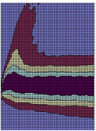
would like to incorporate the information value of these models for decision making and one way to achieve this is through averaging the economic object of interest. As an example of an averaged output which can be used as an input for decision making, Figure 1 presents the higher posterior density re-gions (hpds) for the impulse response function over 60 months for a response in relative UK prices, pt¡p¤t, to a shock in oil prices, pot. This output is

averaged across all models and was produced from 100,000 draws from the full posterior. The intervals plot the boundaries of the 20%, 40%, 60% and 80% hpds. The UK during the period of the sample was a net oil exporter and we see the e¤ect of this re‡ected in the …gure as the distribution of the response path indicates initially that the rest of the world experiences a larger response to an oil price shock than the UK, after which the UK appears to

catch up slightly. However, the greater impact on world prices relative to UK prices seems to persist as after 60 months the path is centred around a slightly negative mode just above negative 1%. This is not a surprising result given the likely exchange rate adjustment in the pound.

********** Figure 1 around here **********

It should be pointed out that these intervals are not comparable with the usual classical con…dence intervals as they incorporate variable uncertainty, parameter uncertainty and model uncertainty. With this extra uncertainty it is sensible then that the intervals containing a given mass will be wider and the mass in any particular region does not have the same interpreta-tion. Trimming the model set of unreasonable models would likely produce smaller intervals. However, the results we present are more informative on the question ‘What will happen to relative prices in the UK if there is an oil price shock?’ as they do not require the addendum: ‘... if this model and these parameter values are correct?’.

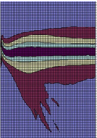
Figure 2 plots the hpds for the impulse response function over 60 months for a response in UK in‡ation,¢pt, to a shock in oil prices, pot, again produced

from 100,000 draws from the posterior. The median response after 60 months shows a moderate increase in the level of in‡ation of around 2.5% and so the median impulse response is about where we would expect it and the 20% and 40% hpds are reasonable.

********** Figure 2 around here **********

An interesting feature of both …gures are the long tails at low lags. This tail behaviour is due entirely to the set of 40 models (out of 97 models) in which oil prices are not constrained to be weakly exogenous. Although these models are given a small (but not negligible) posterior probability (around 8%), their implied response paths are so extreme that they have a noticeable in‡uence upon the marginal distribution of the response.

It is to demonstrate this rather strange behaviour that we have reported the results using the BIC approximation to the posterior probabilities. The same plots of the hpds for the impulse response paths when we used the Laplace approximation or the MCMC estimation do not demonstrate such an extreme diversion in the tail and look similar to what we obtain if we use BIC but exclude the models in which oil prices are not exogenous (e= 1). The

reason for this is that the Laplace and MCMC methods tend to concentrate the mass of the density for the models on fewer models and attribute no mass to the models withe = 1. The behaviour in Figure 2 demonstrates the risks

of conditioning on particular models, but also the risks - also inherent in our approach - of not using a su¢ciently well considered model set.

6 Conclusion.

In this paper we have presented an approach to obtaining inference on the structural features of the vector autoregressive model that are of interest to researchers and for policy analysis. This approach allows the incorporation of uncertainty about the ‘true state of nature’ into the conduct of policy analysis by producing output averaged across models rather than output conditional upon a particular model. The output produced this way allows policy rec-ommendations to be made that are not conditional on a particular model, and thus this model averaging approach provides an important alternative to the more commonly used model selection approach. Speci…cally we provide techniques for estimating marginal likelihoods for models of cointegration, deterministic processes, exogeneity, and overidentifying restrictions upon the cointegrating space. These estimates are derived using a mixture of analyti-cal integration and MCMC or asymptotic approximations to integrals. Two applications of these tools are provided. First for a simple example of a model of Australian money demand and, second, a more complete macroeconomic model of the UK proposed by Garratt,et al..

Very natural extensions of our approach are to include inequality condi-tions in the parameter space of the structural VAR or forms of nonlinearity in the model itself. For instance, in using a SVAR for business cycle analysis one may use prior information on the length and amplitude of the period of oscillation. An example of a possible nonlinear structure that may prove useful is presented in Paap and van Dijk (2003). Systematic use of inequality conditions and nonlinearity implies a more intense use of MCMC algorithms.

7 Acknowledgements

Both authors would like to thank David Hendry, Soren Johansen, Helmut Lutkepohl, and Christopher Sims for helpful discussion on the topic of this