Radiation and Environmental Biophysics manuscript No.
(will be inserted by the editor)
Exposure-lag response associations between lung
cancer mortality and radon exposure in German
uranium miners
Matthias Aßenmacher · Jan Christian Kaiser · Ignacio Zaballa · Antonio Gasparrini · Helmut K¨uchenhoff Received: date / Accepted: date
Matthias Aßenmacher, Helmut K¨uchenhoff Department of Statistics
Ludwig-Maximilians-Universit¨at, 80539 Munich, Germany E-mail: matthias.assenmacher@stat.uni-muenchen.de Jan Christian Kaiser
Institute of Radiation Medicine
Helmholtz Zentrum M¨unchen, 85764 Oberschleissheim, Germany Ignacio Zaballa
Miramar Kalea 11-2, Getxo 48992, Spain Antonio Gasparrini
Department of Social and Environmental Health Research,
London School of Hygiene and Tropical Medicine, 15–17 Tavistock Place, London WC1H 9SH, United Kingdom
Department of Medical Statistics,
London School of Hygiene and Tropical Medicine, Keppel Street, London WC1E 7HT, 1 2 3 4 5 6 7 8 9 10 11 12 13 14 15 16 17 18 19 20 21 22 23 24 25 26 27 28 29 30 31 32 33 34 35 36 37 38 39 40 41 42 43 44 45 46 47 48 49 50
Abstract Exposure-lag response associations shed light on the duration of pathogenesis for radiation-induced diseases. To investigate such relations for lung cancer mortality in the German uranium miners of the Wismut company, we apply distributed lag non-linear models (DLNMs) which offer a flexible de-scription of the lagged risk response to protracted radon exposure. Exposure-lag functions are implemented with B-Splines in Cox models of proportional hazards. The DLNM approach yielded good agreement of exposulag re-sponse surfaces for the German cohort and for the previously studied cohort of American Colorado miners. For both cohorts, a minimum lag of about 2 yr for the onset of risk after first exposure explained the data well, but possibly with large uncertainty. Risk estimates from DLNMs were directly compared with estimates from both standard radio-epidemiological models and biologically-based mechanistic models. For age > 45 yr all models pre-dict decreasing estimates of the Excess Relative Risk (ERR). But at younger age marked differences appear as DLNMs exhibits ERR peaks, which are not detected by other models. After comparing exposure responses for biological processes in mechanistic risk models with exposure responses for hazard ratios in DLNMs, we propose a typical period of 15 yr for radon-related lung carcino-genesis. The period covers the onset of radiation-induced inflammation of lung tissue until cancer death. The DLNM framework provides a view on age-risk
United Kingdom
Centre for Statistical Methodology,
London School of Hygiene and Tropical Medicine, Keppel Street, London WC1E 7HT, United Kingdom 1 2 3 4 5 6 7 8 9 10 11 12 13 14 15 16 17 18 19 20 21 22 23 24 25 26 27 28 29 30 31 32 33 34 35 36 37 38 39 40 41 42 43 44 45 46 47 48 49 50
patterns supplemental to the standard radio-epidemiological approach and to biologically-based modeling.
Keywords uranium miners · radon exposure · lung cancer mortality ·
distributed lag non-linear models·exposure-lag response surface
1 2 3 4 5 6 7 8 9 10 11 12 13 14 15 16 17 18 19 20 21 22 23 24 25 26 27 28 29 30 31 32 33 34 35 36 37 38 39 40 41 42 43 44 45 46 47 48 49 50
1 Introduction
Lung cancer is the most frequent cause of death among all cancer diseases [17]. The predominant risk factor is tobacco smoke followed by anthropogenic environmental radiation exposure, but a good understanding of the biological processes leading to lung cancer is still lacking [1]. Epidemiological risk as-sessment provides a powerful tool to establish statistical associations between exposure to ionizing radiation and late health effects. Radio-epidemiological models rely on a comprehensive description of the radiation risk with appro-priate mathematical functions. In their standard form they apply a response function to the total radiation exposure, which is modified by various predic-tor variables, often called effect modifiers (EMs). For acute exposure these variables include sex, age at exposure and attained age. Risk assessment for protracted exposure requires a detailed exposure history, which has been esti-mated for several carcinogenic agents in the German uranium miners cohort of the Wismut company for the period 1946-1989. Smoking information is only available for part of the cohort [28]. But for exposure to radon and its short lived progeny, which constitutes the second most important lung carcinogen, annual exposures were estimated for each miner from begin to end of em-ployment. Thereafter, cohort members were subject to a mortality follow-up until 2003 as end of follow-up for the present study [27]. Overall, the mortality follow up has been executed until 2013. Lung cancer risks have been studied extensively in the Wismut cohort with complex radio-epidemiological models [25, 47, 49]. Studies on all late health effects are reviewed by Walsh et al. [48].
1 2 3 4 5 6 7 8 9 10 11 12 13 14 15 16 17 18 19 20 21 22 23 24 25 26 27 28 29 30 31 32 33 34 35 36 37 38 39 40 41 42 43 44 45 46 47 48 49 50
Applying the total exposure response with EM adjustment for risk esti-mation represents the quasi-standard approach in radiation epidemiology. It is generally accepted by committees BEIR VI [4], BEIR VII [34], UNSCEAR [45] and ICRP [46] which issue recommendations for radiation protection. On the other hand, this descriptive approach provides little insight into cancer etiology. To make progress here, the present study investigates the distribu-tion of time lags between exposure and outcome. It reflects the duradistribu-tion of disease development, thereby supporting a biologically-based analysis of ob-servational cancer data. Until now, only a few radio-epidemiological studies have addressed this aspect.
In the cohort of Japanese a-bomb survivors, the radiation risk arises from a single event of acute exposure. For leukemia mortality of a-bomb survivors Richardson et al. [38] have reported a peak in the Excess Relative Risk (ERR) 10 yr after exposure. A lognormal lag function with only two parameters pro-vided a good description of the data. For protracted exposure, a lagged re-sponse cannot be gleaned directly from incidence data but can be uncovered by disentanglement of the exposure-lag response. Several approaches have been tested on the cohort of Colorado Plateau uranium miners, which exhibits ex-posure patterns similar to the Wismut cohort but with additional records for smoking habits [42]. Pertinent studies are built on the assumption, that ex-posure in short constant age intervals contributes additively to the radiation risk albeit with differential weight [6, 13, 20].
1 2 3 4 5 6 7 8 9 10 11 12 13 14 15 16 17 18 19 20 21 22 23 24 25 26 27 28 29 30 31 32 33 34 35 36 37 38 39 40 41 42 43 44 45 46 47 48 49 50
Hauptmann et al. [20] analyzed exposure-lag relationships using spline weight functions. Deviating from the standard radio-epidemiological approach as described above, they applied a linear risk response to the exposure rate1.
Armstrong [2] and Berhane et al. [6] extended this scheme to accommodate time-varying exposure.
Gasparrini [12, 13] applied a more general framework for the analysis of exposure-lag response associations in the cohort of Colorado Plateau uranium miners usingdistributed lag non-linear models(DLNMs). Such models are con-structed by a flexible bivariateexposure-lag response surface, which maintains the linearity of model parameters. Consistent with previous studies [6, 20] Gas-parrini [13] estimated a similar shape for the lag response curve, which was constructed with quadratic B-splines.
Implemented as a package in R [36], the DLNM framework offers convenient versatility to describe model non-linearities and distributed lag effects [12]. It features an algebraic definition of standard errors, confidence intervals and tests, allows for a flexible use of different functions for each dimension and provides a well-designed tool for interpreting results.
Zaballa and Eidem¨uller [51] applied a biologically-based Two Stage Clonal Expansion (TSCE) model to the Wismut cohort. Their mechanistic analysis was concerned with biological aspects of lung carcinogenesis such as oncogenic mutations and the growth dynamics of pre-cancerous lesions. As biological 1 In the standard radio-epidemiological approach exposure response is related to cumu-lative exposure, whereas exposure response in the DLNM framework is related toexposure rate. 1 2 3 4 5 6 7 8 9 10 11 12 13 14 15 16 17 18 19 20 21 22 23 24 25 26 27 28 29 30 31 32 33 34 35 36 37 38 39 40 41 42 43 44 45 46 47 48 49 50
target of radon exposure they proposed clonal expansion of initiated cells in-creased by radiation-induced inflammation. The mechanistic TSCE model is fully capable of providing risk estimates for comparison with standard risk models. Thus, to put the results of the TSCE model into perspective, they applied a modified version of the preferred ERR model from Walsh et al. [47] as reference.
In the cohort of Colorado miners about 260 lung cancers cases have been recorded until end of 1982, compared to about 3000 cases in the Wismut cohort followed up until 2003. As the largest cohort of uranium miners in the world to date, the Wismut cohort offers a unique opportunity to validate the results of Gasparrini [13] for the Colorado Plateau uranium miners. With the present study we examine response functions of the hazard ratio related to both annual radon exposure and time since exposure. Second, estimates of the ERR from our preferred DLNM are compared with results from both mechanistic models and standard radio-epidemiological models applied in the study of Zaballa and Eidem¨uller [51]. Our main interest here is to assess the ability of risk models to represent plausible exposure-lag response associations. Finally, by comparing results from DLNMs and biologically-based risk models, we speculate on the duration of development for radon-related lung cancer.
1 2 3 4 5 6 7 8 9 10 11 12 13 14 15 16 17 18 19 20 21 22 23 24 25 26 27 28 29 30 31 32 33 34 35 36 37 38 39 40 41 42 43 44 45 46 47 48 49 50
2 Materials and Methods
2.1 The Wismut Cohort
In March 2016 we obtained access to the Wismut cohort data set from the Ger-man Federal Office for Radiation Protection (Bundesamt f¨ur Strahlenschutz (BfS)) by transfer agreement. The full data set comprises 58,987 men who were formerly employed at the Wismut company in the years from 1946 to 1989. Radiation exposure was estimated by using a detailed job-exposure matrix (JEM), which includes information on exposure to radon and its progeny in WLM, external radiation in units of mSv and long-lived radionuclides (235U, 238U) in units of kBq h/m3. The JEM provides exposure values for each
cal-endar year of employment between 1946-1989, each place of work and each type of job. More than 900 different jobs and 500 different working places were evaluated for this purpose. Radon (222Rn) measurements in the Wismut
mines were carried out from 1955 onwards. For the period from 1946-1954, radon concentrations were estimated retrospectively by an expert group based on measurements from 1955, taking into account specific mining conditions in the early period. From 1955-1965 about 57,000 radon gas measurements were taken in Saxonian underground mines, from 1966-1990 about 140,000 radon progeny measurements were performed. The corresponding numbers for Thuringian underground mines are about 39,000 radon measurements between 1955-74, and about 160,000 radon progeny measurements from 1975-1990. For each calendar year and each mining object individual exposure estimates were
1 2 3 4 5 6 7 8 9 10 11 12 13 14 15 16 17 18 19 20 21 22 23 24 25 26 27 28 29 30 31 32 33 34 35 36 37 38 39 40 41 42 43 44 45 46 47 48 49 50
assigned to all cohort members. More details on exposure estimation and un-certainty assessment are given in the reports of Lehmann et al. [30, 31] and of K¨uchenhoff et al. [29].
Due to missing values for silica dust exposure 292 members were excluded, so that 58,695 workers contributed to the present analysis. A miner was con-sidered at risk from date of first employment until date of death, date of loss to follow-up or end of follow-up (December 31, 2003). In total, 20,757 deaths occurred as 35.4% of the full cohort of which 2,996 deaths (5.1%) were at-tributed to lung cancer. For a more circumstantial description of the Wismut cohort see ref. [27].
2.2 The Cox model
Theory
For risk assessment we apply an extension of Cox’s model of proportional hazards to allow for non-linearity and lagged effects in exposure-related co-variables using the algebraic notation
λ(t, x, z, cal, abe) =λ0(t)·exp [sx(x, t)
+sz(z, t) +γ cal+δ abe].
(1)
withsx(radon) andsz (silica dust) as non-linear exposure covariables, calen-dar timecal(centered around the year 1970) and the age at begin of employ-mentabeas linear covariables.
1 2 3 4 5 6 7 8 9 10 11 12 13 14 15 16 17 18 19 20 21 22 23 24 25 26 27 28 29 30 31 32 33 34 35 36 37 38 39 40 41 42 43 44 45 46 47 48 49 50
Inference
Inference in the Cox model is performed via the partial likelihood approach, using Efron’s method [9] for tie handling, which allows to skip the estimation of the nuisance parameter λ0(t) to reduce complexity [8]. Risk estimates are
expressed as hazard ratios (HRs). The statistical analysis was performed using the packagessurvival[43, 44] anddlnm [12] within the statistical softwareR
[36, 40]. The figures were created using the packageggplot2[50].
2.3 The DLNM framework
As the analysis is based on an approach introduced by Gasparrini and col-leagues [13–15] we will give a brief summary of the mathematical background and the inference methods. While Gasparrini et al. [14] are mainly concerned with time series analysis, Gasparrini [13] applies the methodology to analyze time-to-event data with the Cox model. Gasparrini et al. [15] focus on the ex-tension to a penalized framework. Bender et al. [5] use a piecewise exponential model for a flexible analysis of lagged effects. We start with an introduction of the simpler distributed lag models (DLMs), which are then extended to accommodate more complex non-linearities [13].
Distributed lag models (DLMs)
DLMs describe the lag response relationship for a linear effect of exposure, understood here as annual rates for exposure to radon and its short-lived
1 2 3 4 5 6 7 8 9 10 11 12 13 14 15 16 17 18 19 20 21 22 23 24 25 26 27 28 29 30 31 32 33 34 35 36 37 38 39 40 41 42 43 44 45 46 47 48 49 50
progeny. Gasparrini [13] describes the relation in the following form s(x, t) = Z L `0 xt−`·w(`) d` (2a) ≈ L X `=`0 xt−`·w(`), (2b)
wherew(`) is the so-called lag response function.
In Eq. (2a), L−`0 defines the period while exposure has an effect on
outcome. Eq. (2b) is an approximation of the integral (2a). An optimal value for the minimum lag `0 will be searched in the present study. The maximum
lagLis confined to 40 yr after exposure as in ref. [13], although some cohort members are followed up for 57 years.
Expressings(x, t) in matrix notation yields
s(x, t;η) =q>i,tCη=w>i,tη, (3) where qi,t = (xi,t−`0, ..., xi,t−`, ..., xi,t−L)
> and C as a transformation of the
lag vector`with a vector of dimensionυ>` defining the basis functions. So Eq. (3) is the vectorial representation of Eq. (2a) with adjustable parametersηas coefficients for B-Splines.
Distributed lag non-linear models (DLNMs)
Allowing for non-linearity inxand giving up the assumption of independence off(.) andw(.) yields s(x, t) = Z L `0 f·w(xt−`, `) d` (4a) ≈ L X `=`0 f·w(xt−`, `), (4b) 1 2 3 4 5 6 7 8 9 10 11 12 13 14 15 16 17 18 19 20 21 22 23 24 25 26 27 28 29 30 31 32 33 34 35 36 37 38 39 40 41 42 43 44 45 46 47 48 49 50
wheref·w(xt−`, `) is a truly bivariate function inxand int. This constitutes an exposure-lag response surface [13], which is parameterized with a special tensor product, calledcross-basis [2].
By defining2
Ai,t= Ri,t⊗1>υ`
1>υx⊗C
, (5)
the cross-basis function can be written as
s(x, t;η) = 1>L−`0+1Ai,tη=w>i,tηx. (6) Similar toCin Eq. (3),Ri,t is constructed by transformingqi,twith a vector of dimensionυx. The identifiabilty issues mentioned by Gasparrini [13] do not apply here as we do not include intercepts in the basis functions for exposure covariablesxandz insx(x, t) andsz(z, t), respectively.
2.4 Model selection
Model selection is performed with goodness-of-fit measured by the Akaike information criterion (AIC) and the Bayesian information criterion (BIC). These two criteria are given as
AIC =−2· L(ˆηx,ηˆz,ˆγ,δ) + 2ˆ ·df (7a)
BIC =−2· L(ˆηx,ηˆz,ˆγ,δ) + ln(n)ˆ ·df, (7b)
where n is the number of uncensored events (i.e. lung cancer deaths) and df is the degree of freedom (or model parameters). Parameters estimates are
2 ⊗denotes the Kronecker product, whiledenotes the Hadamard product 1 2 3 4 5 6 7 8 9 10 11 12 13 14 15 16 17 18 19 20 21 22 23 24 25 26 27 28 29 30 31 32 33 34 35 36 37 38 39 40 41 42 43 44 45 46 47 48 49 50
calculated for B-spline coefficients in the exposure-lag response relations for radon ˆηxand silica dust ˆηz, and for adjustment to calendar year ˆγand age at begin of exposure ˆδ.
In the primary analysis to this study (Master thesis of Matthias Aßen-macher [3]) some 50 models have been fitted. We chose model selection by AIC as the method of choice although slight over-fitting can come with it. On the other hand, BIC selection produced too sparse models, which tend to overlook important features of the data. In addition, we report results of LRTs, to support the findings obtained by comparison of AIC vs. BIC, where possible.
To avoid biologically implausible exposure-lag response surfaces we applied an additionalcriterion of wiggliness. In the lag response relationship, curves with wiggly courses are not accepted. Wiggly curves are defined as having more than one change in slope from positive to negative or vice versa. The criterion is motivated by the assumption that protracted exposure of limited duration causes health effects, which peak after a typical time since exposure and decline thereafter.
2.5 Descriptive ERR model of Zaballa and Eidem¨uller
For comparison with the results of our study we apply the descriptive ERR model of Zaballa and Eidem¨uller [51]
ERRr=βrD 1 +αt1(tsme−11) +αt2(tsme−11)2 (8) · exp [−αa(a−44)−αr(davg−32.4)] 1 2 3 4 5 6 7 8 9 10 11 12 13 14 15 16 17 18 19 20 21 22 23 24 25 26 27 28 29 30 31 32 33 34 35 36 37 38 39 40 41 42 43 44 45 46 47 48 49 50
with central ERR coefficient βr for cumulative radon exposure and EMs for time since median exposuretsme, attained ageaand mean exposure ratedavg expressed in working level months per year (WLM/yr). Maximum likelihood estimates for model parameters are given in Table 4 of Zaballa and Eidem¨uller [51]. Note, that for their biologically-based TSCE model no closed analytical form can be given.
1 2 3 4 5 6 7 8 9 10 11 12 13 14 15 16 17 18 19 20 21 22 23 24 25 26 27 28 29 30 31 32 33 34 35 36 37 38 39 40 41 42 43 44 45 46 47 48 49 50
3 Results
We systematically explored a large number of models to determine our pre-ferred DLNM. The model design is successively revised by variation of the cross basis in Eq. (6). Each model is assessed by its goodness-of-fit and biological plausibility. Suitable adjustments for silica dust and minimum lag`0for radon
exposure have been examined with simpler DLMs. To limit the number of test calculations, these adjustments have been retained for the more complex DLNMs without modification. Results of our investigations are summarized here, more detailed information is given in the Appendix and in the primary analysis [3].
3.1 DLMs
DLMs rely on a linear relationship of the response to the annual radon exposure ratext−`given in Eq. (2b). For the lag response functionwx(`) various forms have been tested as reported in Appendix A.1. At the onset, the HR depen-dence on exposure to silica dust has been determined. The exposure-response functionf(zt−`) for silica dust is specified as a linear threshold function, and the lag-response functionwz(`) is chosen as piecewise constant with two cut-off points. The minimum lag`0 was set to 2 yr. The lag response association
of our preferred DLM L5 is shown in Fig. A2. Table A1 summarizes proper-ties and goodness-of-fit (includingp-values of LRTs) for a selected number of DLMs. 1 2 3 4 5 6 7 8 9 10 11 12 13 14 15 16 17 18 19 20 21 22 23 24 25 26 27 28 29 30 31 32 33 34 35 36 37 38 39 40 41 42 43 44 45 46 47 48 49 50
3.2 DLNMs
The evaluation of DLMs already showed that B-Splines of higher degrees are not suited for modeling the lag response. Consequently, B-Splines of degrees five and six are no longer considered [3]. B-Splines of degree one are discarded a-priori as they possibly oversimplify the true underlying relationship. Con-cerning the knots and their placement, up to five knots on equally spaced quantiles of the lag distribution were chosen.
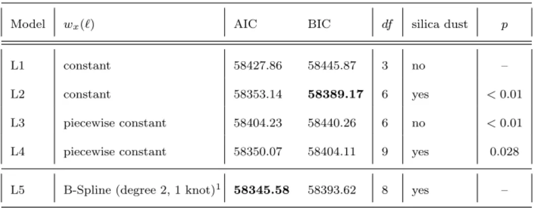
For the characterization of the exposure-response function, B-Splines are applied as well. In this case, B-Splines of degree two, three and four in com-bination with zero to five knots at equally spaced quantiles of the exposure distribution are taken into consideration. The AIC-selected models character-ize the exposure response well. The 20 AIC-best models all include a B-Spline of degree two with two knots at 33.3% and the 66.6% quantiles of the exposure distribution. Within these models, considerable variation was observed for the lag response, but none of the AIC-best models contains a B-Spline with more than three knots. Table 1 summarizes the properties and goodness-of-fit for selected DLNMs, which all apply the same B-Splines of degree two for the preferred non-linear risk response to annual radon exposure. Compared to the preferred DLM L5 nearly all models improve the AIC by about hundred points.
1 2 3 4 5 6 7 8 9 10 11 12 13 14 15 16 17 18 19 20 21 22 23 24 25 26 27 28 29 30 31 32 33 34 35 36 37 38 39 40 41 42 43 44 45 46 47 48 49 50
Table 1 Properties and goodness-of-fit for DLNMs NL1 to NL4 with exposure-(rate)-responsef(xt−`) constructed from B-splines of degree 2 with 2 knots at 1.6 WLM/yr and
16.5 WLM/yr, for the lag responsewx(`) the knot is placed at 20 yr,dfdenotes the number
of model parameters, lowest values for AIC and BIC in bold. We also carried out LRTs where NL2 was tested against NL1 (p < 0.01) and NL4 (p = 0.205). The tests indicate a superior goodness-of-fit of NL2 compared to NL1, but no superiority compared to NL4 (despite the inclusion of the intercept). NL4 is our preferred model.
Model wx(`) AIC BIC df
NL1 constant 58241.75 58295.79 9
NL2 B-Spline (degree 2, 1 knot, intercept) 58234.52 58360.62 21 NL3 B-Spline (degree 2, 1 knot, right-constrained) 58295.72 58349.77 9 NL4 B-Spline (degree 2, 1 knot) 58232.44 58334.52 17
Minimum lag period
In the primary analysis to this study special attention has been given to the characterization of the minimum lag period for risk onset [3]. Minimum lag`0
was defined as the time after (first) exposure when the HR exceeds a biolog-ically plausible threshold of one. Using a heuristic method, some 50 models have been examined with a minimum lag varying between 0 and 5 yr. Based on goodness-of-fit, models with a minimum lag between 2 and 3 yr yielded a good data description. Models with longer minimum lag provided markedly inferior fits.
We reexamined the estimation of `0 by considering model NL2 which
al-lowed for flexible minimum lags depending on exposure rate as shown in Fig.
1 2 3 4 5 6 7 8 9 10 11 12 13 14 15 16 17 18 19 20 21 22 23 24 25 26 27 28 29 30 31 32 33 34 35 36 37 38 39 40 41 42 43 44 45 46 47 48 49 50
1. In model NL2 the intercept varies weakly with exposure rate and is com-patible with a 2 yr minimum lag. Model NL4 with a fixed minimum lag at 2 yr yields a slightly lower AIC than model NL2, but with four intercept-related parameters less its BIC is considerably lower (Table 1).
1.0 1.1 1.2
0 10 20 30 40
Time since exposure (yr)
HR Exposure rate 30 WLM/yr 50 WLM/yr 100 WLM/yr 150 WLM/yr 200 WLM/yr
Fig. 1 Lag-response curves for the hazard ratio (HR) of model NL2 for exposure rates of 30 WLM/yr to 200 WLM/yr, model NL2 was used to estimate minimum lags.
Behavior long after exposure
To investigate the behavior long after exposure, the lag-response function in DLNM NL3 was right-constrained to HR = 1 at time since exposure 40 yr. Compared to models NL4 and NL2 without right-constraint the information criteria AIC and BIC were markedly increased, suggesting a significant residual lung cancer risk more than 40 yr after exposure (Table 1). Figs. A3 and A4 in the Appendix depict lag response curves, exposure response curves and the complete exposure-lag-response surface of model NL3.
1 2 3 4 5 6 7 8 9 10 11 12 13 14 15 16 17 18 19 20 21 22 23 24 25 26 27 28 29 30 31 32 33 34 35 36 37 38 39 40 41 42 43 44 45 46 47 48 49 50
Preferred DLNM
After assessing DLNMs NL1 - NL4 based on goodness-of fit and biological plausibility, we choose NL4 as our preferred DLNM. Model NL4 satisfies the criterion of wiggliness and has an AIC of about 113 points lower than the preferred DLM L5 (Table 1, Fig. A2 in the Appendix). It contains a cross-basis with a B-Spline of degree two with two knots for the exposure response function at 1.6 WLM/yr and 16.5 WLM/yr, and a B-Spline of degree two with one knot at a lag of 20 years for the lag response. Estimates for the cross-basis coefficients are given in Table A3 in the Appendix.
3.3 Age-risk patterns of the preferred DLNM
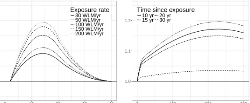
The exposure-lag-response surface is shown in Fig. 2 and selected lag-response curves and exposure-response curves are depicted in the upper panels of Fig. 3. Peak hazard ratios appear about 15 yr after exposure to any annual radon exposure rate from 5 WLM/yr to 300 WLM/yr. The lag-response flattens for time since exposure>30 yr but does not vanish at the end of the lag period L= 40 yr.
The exposure response increases sharply below an exposure rate of about 20 WLM/yr and then reverts to a smaller slope until about 200 WLM/yr. For exposure>200 WLM/yr a small drop in the exposure response is observed for time since exposure<30 yr. But for larger lag times the increase continues. At very low exposure rates<5 WLM/yr hazard ratios become smaller than one.
1 2 3 4 5 6 7 8 9 10 11 12 13 14 15 16 17 18 19 20 21 22 23 24 25 26 27 28 29 30 31 32 33 34 35 36 37 38 39 40 41 42 43 44 45 46 47 48 49 50
Such protective effects at low exposure rates have been reported for animal experiments [21]. However, they are not in the focus of the present study and may well be attributed to mathematical artifacts of knot placement. Estimates for confounders age at begin of employment, calendar year and silica dust exposure for the preferred DLNM NL4 are given in Table A2 and Fig. A5 in the Appendix. Exposure r ate (WLM/yr) 0 50 100 150 200 250 300 Time since e xposure (yr) 5 10 15 20 25 30 35 40 HR 0.90 0.95 1.00 1.05 1.10 1.15 1.20 1.25
Fig. 2 Exposure-lag-response surface for the hazard ratio (HR) of the preferred DLNM NL4, two solid lines along the surface delineate a lag response curve at exposure 70 WLM/yr and an exposure response curve at time since exposure 15 yr, at exposure rates<5 WLM/yr the HR becomes<1. 1 2 3 4 5 6 7 8 9 10 11 12 13 14 15 16 17 18 19 20 21 22 23 24 25 26 27 28 29 30 31 32 33 34 35 36 37 38 39 40 41 42 43 44 45 46 47 48 49 50
1.0 1.1 1.2 1.3
0 10 20 30 40
Time since exposure (yr)
HR Exposure rate 30 WLM/yr 50 WLM/yr 100 WLM/yr 150 WLM/yr 200 WLM/yr 1.0 1.1 1.2 1.3 0 100 200 300
Exposure rate (WLM/yr)
HR
Time since exposure
10 yr 15 yr 20 yr 30 yr 1.0 1.1 1.2 1.3 0 10 20 30 40
Time since exposure (yr)
HR Exposure rate 30 WLM/yr 50 WLM/yr 100 WLM/yr 150 WLM/yr 200 WLM/yr 1.0 1.1 1.2 1.3 0 100 200 300
Exposure rate (WLM/yr)
HR
Time since exposure
10 yr 15 yr 20 yr 30 yr
Fig. 3 Selected lag-response curves of the hazard ratio (HR) for radon exposure rates between 30 WLM/yr and 200 WLM/yr (left panels) and exposure-response curves of the HR for time since exposure between 10 yr and 30 yr (right panels) for our preferred DLNM NL4 (top panels) to model 8 by Gasparrini [13] (bottom panels).
Baseline rates from the preferred DLNM NL4 are displayed in Fig. A6 of the Appendix for age intervals of five years and six calendar year periods between 1946 - 2003. Baseline rates from both the mechanistic and the de-scriptive models exhibit an attenuation or even a decrease at old age (results not shown). Compared to baseline rates from the preferred DLNM NL4 they possibly provide a more accurate description of the male lung cancer mortality in Germany but a deeper investigation of baseline rates is beyond the scope of the present study.
1 2 3 4 5 6 7 8 9 10 11 12 13 14 15 16 17 18 19 20 21 22 23 24 25 26 27 28 29 30 31 32 33 34 35 36 37 38 39 40 41 42 43 44 45 46 47 48 49 50
3.4 Exposure scenarios
To compare risk estimates of our preferred DLNM NL4 with those of the stan-dard radio-epidemiological ERR model (cited in Eq. 8) and the biologically-based TSCE model, both from Zaballa and Eidem¨uller [51], we consider sce-narios motivated by the distribution of covariables age of death, age at median exposure, exposure duration, exposure rate and cumulative lifetime exposure summarized in their Table 5. Birth year 1930 was assumed for a miner with-out silica exposure, the period of exposure was centered around median age 26 yr in 1956. For the scenario calculations 12.5 WLM/yr was chosen as min-imal exposure rate, although mean exposure rates of 7 WLM/yr for miners employed after 1955 and 1.4 WLM/yr for miners employed after 1959 were markedly lower. However, for such low exposure rates the exposure response of the preferred DLNM NL4 is burdened with considerable uncertainty and should not be applied (Figs. 2 and 3).
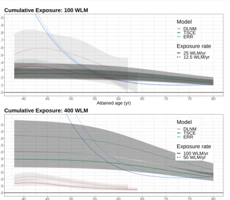
For a scenario of constant cumulative exposure 100 WLM and 400 WLM with duration of 4 yr and 8 yr lung cancer mortality was considered for attained age from 40 - 80 yr, corresponding to calendar years 1970 - 2010. Fig. 4 depicts estimates for the age dependence of the ERR. Due to the DLNM construction for Cox regression in Eq. 1, the corresponding ERR =λ(x=d)/λ(x= 0)−1 = exp[sx(x=d, t)]−1 depends only on exposure ratedand time since exposure t, whereas dependencies on calendar yearcaland age at begin of employment abecancel out.
1 2 3 4 5 6 7 8 9 10 11 12 13 14 15 16 17 18 19 20 21 22 23 24 25 26 27 28 29 30 31 32 33 34 35 36 37 38 39 40 41 42 43 44 45 46 47 48 49 50
0.0 0.1 0.2 0.3 0.4 0.5 0.6 0.7 0.8 0.9 1.0 40 45 50 55 60 65 70 75 80
Attained age (yr)
ERR Model DLNM TSCE ERR Exposure rate 25 WLM/yr 12.5 WLM/yr Cumulative Exposure: 100 WLM 0.0 0.5 1.0 1.5 2.0 2.5 3.0 3.5 4.0 4.5 5.0 40 45 50 55 60 65 70 75 80
Attained age (yr)
ERR Model DLNM TSCE ERR Exposure rate 100 WLM/yr 50 WLM/yr Cumulative Exposure: 400 WLM
Fig. 4 Estimates of the ERR depending on attained age for cumulative exposure to 100 WLM at exposure rates 12.5 WLM/yr and 25 WLM/yr (upper panel) and for cumulative exposure to 400 WLM at exposure rates 50 WLM/yr and 100 WLM/yr (lower panel) at age of median exposure 26 yr for the preferred DLNM (red), the TSCE model (green) and the ERR model (blue), shaded areas display 95% CIs of the preferred DLNM (light gray) and the TSCE model (dark gray).
For a scenario of constant exposure rates 12.5 WLM/yr and 100 WLM/yr Fig. 5 shows estimates of the ERR for attained age 60 yr in 1990 depending on radon exposure accumulated by increasing exposure duration up to 12 yr. Risk dependence on cumulative exposure is considered here to assess the range of applicability for the linear no-threshold (LNT) paradigm in radiation pro-tection. 1 2 3 4 5 6 7 8 9 10 11 12 13 14 15 16 17 18 19 20 21 22 23 24 25 26 27 28 29 30 31 32 33 34 35 36 37 38 39 40 41 42 43 44 45 46 47 48 49 50
0.0 0.1 0.2 0.3 0.4 0.5 0.6 0.7 0 25 50 75 100 125 150 Cumulative Exposure (WLM) ERR Model DLNM ERR TSCE
Exposure rate: 12.5 WLM/yr
0.00 0.25 0.50 0.75 1.00 1.25 1.50 1.75 2.00 2.25 2.50 0 150 300 450 600 750 900 1050 1200 Cumulative Exposure (WLM) ERR Model DLNM ERR TSCE
Exposure rate: 100 WLM/yr
Fig. 5 Estimates of the ERR depending on cumulative radon exposure for the preferred DLNM (red), the TSCE model (blue) and the ERR model (green) for scenarios with age at median exposure 26 yr, attained age 60 yr and constant exposure rates 12.5 WLM/yr (upper panel), 100 WLM/yr (lower panel) for exposure duration up to 12 yr, shaded areas display 95% CIs of the preferred DLNM (light gray) and the TSCE model (dark gray), for the lower exposure rate 12.5 WLM/yr DLNM and TSCE model give the same result. 1 2 3 4 5 6 7 8 9 10 11 12 13 14 15 16 17 18 19 20 21 22 23 24 25 26 27 28 29 30 31 32 33 34 35 36 37 38 39 40 41 42 43 44 45 46 47 48 49 50
4 Discussion
4.1 Comparison with the preferred DLNM for the Colorado cohort
Fig. 3 compares lag-response and exposure-response curves from our preferred DLNM NL4 with those from the preferred DLNM model 8 for the Colorado cohort [13]. Exposure-lag response relationships from both studies produced similar estimates for hazard ratios in the range between 1.2 - 1.3. Despite missing adjustment for smoking in the Wismut cohort and missing adjustment for silica dust in the Colorado cohort, estimates from both cohorts agree very well. Previous studies pointed to sub-multiplicative response of the relative risk to joint action of radon and smoking with a reduction of the radon risk by some 20% [32, 33]. We observed a similar effect of on average 16% reduction for interaction between exposure to silica dust and radon.
The shape of the lag response curves exhibits similar features. Estimates of peak risk between 10-15 yr after exposure are broadly consistent. However, the lack of evidence of a risk more than 35 yr after radon exposure in the Colorado cohort may be related to a small number of cases contributing for large time since exposure. In the Wismut cohort the radon risk persists even after a time lag of 40 yr, which is biologically more plausible.
The majority of uranium miner studies routinely rely on 5 yr lags for cumulative exposure (see e.g. refs. [42] for Colorado miners and [28, 25, 47] for Wismut miners). Yet Fig. 3 shows, that HRs from DLNMs at 5 yr after exposure may have already reached half the maximum risk in some cases.
1 2 3 4 5 6 7 8 9 10 11 12 13 14 15 16 17 18 19 20 21 22 23 24 25 26 27 28 29 30 31 32 33 34 35 36 37 38 39 40 41 42 43 44 45 46 47 48 49 50
Application of 5 yr lags could underestimate the riskshortlyafter first exposure but risks occurring much later than 5 yr after exposure are still adequately described.
The non-linear exposure response association to annual radon exposure rates exhibits break points between 20 WLM/yr (present study) and 50 WLM/yr (Gasparrini [13]) which mark a change to reduced slope (Fig. 3). The biological meaning of break points must not be over-interpreted since they are intrin-sic features in B-Splines. A natural logarithm describes the exposure response almost equally well [3].
4.2 Comparison with standard radio-epidemiological and biologically-based risk models
In Fig. 4 all three models predict a decreasing risk at old age but with markedly different trends. The ERR from the DLNM peaks at about 43 yr as expected from the lag response curves. The TSCE model does not exhibit a maximum risk but the risk decays smoothly from a constant plateau. The course of the risk from the ERR model is dominated by an exponential decay at young ages, which is mitigated by a time-since-exposure effect at old ages. Whereas for cumulative exposure 100 WLM all models produce ERR estimates in the same range, for cumulative exposure 400 WLM the ERR estimates of the DLNM are significantly lower consistent with results shown in Fig. 5.
While the ERR model includes the LNT assumption in its design, responses to the cumulative radon exposure in the TSCE model and the DLNM model
1 2 3 4 5 6 7 8 9 10 11 12 13 14 15 16 17 18 19 20 21 22 23 24 25 26 27 28 29 30 31 32 33 34 35 36 37 38 39 40 41 42 43 44 45 46 47 48 49 50
can deviate from linearity if suggested by fits to the data. In DLNMs the HR is roughly proportional to exp(βD), which for small cumulative exposureDis approximated by a linear response 1+βD. In Fig. 5 a low exposure rate of 12.5 WLM/yr leads to 150 WLM cumulative exposure at maximum. For cumulative exposure up to this maximum linearity is supported by all three models. For higher cumulative exposure up to 1200 WLM, which is caused by an exposure rate of 100 WLM/yr, the response of the TSCE model shows a clear upward curvature, which is weakly reflected by the DLNM. This behavior is in line with findings for the Wismut cohort where non-linearity for ERR models has been tested by Walsh et al. [47] (see the discussion of their Fig. 1). Statistical significance of a quadratic term for cumulative exposure disappeared after adjusting for exposure rate.
An analysis with descriptive Poisson regression models yielded a central estimate for ERR/100 WLM of 1.06 (95% CI: 0.69; 1.42) [47]. The ERR was adjusted for EMs median age at exposure centered at 33 yr, time since median exposure centered at 11 yr, and exposure rate centered at 2.7 WL. Zaballa and Eidem¨uller [51] reported a central estimate of 1.28 (95% CI: 0.81; 1.77) from their ERR model using the same EMs time since median exposure and exposure-rate. We find a corresponding estimate of 0.25 (95% CI 0.18; 0.31) for a rate of 32.4 WLM/yr (= 2.7 WL) and time since exposure between 9.5 yr and 12.5 yr from our preferred DLNM. Our estimate is much lower than estimates from TSCE model and from the descriptive ERR model, which
1 2 3 4 5 6 7 8 9 10 11 12 13 14 15 16 17 18 19 20 21 22 23 24 25 26 27 28 29 30 31 32 33 34 35 36 37 38 39 40 41 42 43 44 45 46 47 48 49 50
assumes a linear-quadratic attenuation effect for time since exposure in the exponent (Eq. 8).
4.3 Onset and duration of development for radon-related lung cancer
Drawing conclusions on lung cancer etiology from radio-epidemiological mod-els, which merely rely on statistical associations, has strict limitations [18, 39]. As a necessary condition the biological concept of cancer development must be specified [7]. For radiation-induced carcinogenesis the biologically based TSCE model provides such a concept and has been successfully applied to a wide range of radio-epidemiological data sets [41]. By jointly analyzing results from DLNMs and TSCE models, we can gain some insight into the duration of development for radon-related lung cancer.
We interpret the latency period tlat as the time span between the appear-ance of the first malignant cell to the time to death. This interpretation is com-monly used in biologically-based modeling of lung carcinogenesis [16, 33, 51]. Latencytlatis not yet accessible by direct measurement and depends strongly on model assumptions. In the present study the minimum lag (or intercept)l0
is understood as the time period after which first exposure starts to increase the value for the hazard ratio above one. An estimate for the minimum lagl0
can be gleaned from observational data with some uncertainty. For example, Heidenreich et al. [22] estimated a minimum lag of 3 yr after exposure for post-Chernobyl thyroid cancer incidence. According to the mechanistic model of carcinogenesis for miners cohorts some time passes after first exposure to
1 2 3 4 5 6 7 8 9 10 11 12 13 14 15 16 17 18 19 20 21 22 23 24 25 26 27 28 29 30 31 32 33 34 35 36 37 38 39 40 41 42 43 44 45 46 47 48 49 50
develop the first malignant cell [33, 51]. With these assumptions minimum lag l0 >must always exceed (minimum) latencytlat. But as we argue below both periods may be rather short.
Minimum lag for the onset of risk
Comprehensive investigations in the present study and in the Colorado study [13] suggest a minimum lag of 2 yr for onset of the radiation risk. Although the study of Berhane et al. [6] did not aim to determine the minimum lag period, their Fig. 3 supports a minimum lag of 2-3 yr by extrapolation of the HR in thelow exposure category.
It is instructive to apply findings from biologically-based modeling of lung tumor growth for the assessment of results from the observational studies. In the analysis of Geddes [16] minimal latencies were calculated under the as-sumption of an exponential tumor growth model, where growth starts with a single malignant cell. Exponential growth functions have been fitted to tu-mors with minimal diameter of 1 cm, corresponding to about 109 cells. A tumor eventually becomes fatal with a size of 10 cm or 1012cells (Geddes [16],
Table I). Below size 1 cm, growth dynamics is inferred by extrapolation and may not necessarily be correct, because cancer stem cells develop from small precursor lesions which do not exhibit the molecular spectrum of a full blown tumor. For lung adenocarcinoma, atypical adenomatous hyperplasia (AAH) are considered as putative precursor lesions [35]. Often AAH are converted to malignancy by a second mutation in a tumor suppressor gene, i.e. TP53. In
1 2 3 4 5 6 7 8 9 10 11 12 13 14 15 16 17 18 19 20 21 22 23 24 25 26 27 28 29 30 31 32 33 34 35 36 37 38 39 40 41 42 43 44 45 46 47 48 49 50
fact, mechanistic models of carcinogenesis for miners cohorts are based on this assumption [33, 51]. AAH are about 5 mm large, when they possibly become malignant. A back-of-the-envelope calculation suggests an AAH would turn into a fatal tumor after about 13 doublings. Based on the doubling times of Geddes [16] (Table II) short latency periods would be conceivable, in partic-ular, if the carcinogenic effect of radon exposure targets advanced precursor lesions as in the mechanistic miners models. Applying the lowest estimate for a doubling time of 29 d pertaining to small (oat) cell carcinoma results in a latency period of about 1 yr well below the minimum lag of 2 yr. As an impli-cation, the minimum period for the appearance of a second (or transforming) oncogenic mutation after first exposure would be also 1 yr.
Hence, simple consideration of tumor growth dynamics confers biological plausibility to a minimal lag time of about 2 yr, which has been found in observational studies.
Duration of development for radon-related lung cancer
Analysis of both experimental animal data and miner cohorts with mechanis-tic TSCE models consistently revealed as the main radon target clonal growth, which is enhanced by reduced inactivation of initiated cells [11, 21, 24, 33, 51]. The growth curves are characterized by linear increase at low exposure rates which is followed by leveling at high exposure rates. Radiation-induced in-flammation has been found to increase clonal expansion in animal studies [19].
1 2 3 4 5 6 7 8 9 10 11 12 13 14 15 16 17 18 19 20 21 22 23 24 25 26 27 28 29 30 31 32 33 34 35 36 37 38 39 40 41 42 43 44 45 46 47 48 49 50
Thus, it is plausible to propose inflammation of the lung epithelium as the underlying mechanism for non-linear behavior of clonal growth [51].
Luebeck et al. [33] estimated a mean latency period of 9 yr from the appear-ance of the first cappear-ancer cell to lung cappear-ancer death for all histologic lung cappear-ancer types combined. Geddes [16] (Table IV) reports a mean latency of 11 years similar to ref. [33]. Results of the present study suggest that onset of radon-induced lung inflammation shapes the exposure response curves of DLNMs starting about 2 yr after first exposure with a mean lag of 15 yr. Comparing the estimates for mean lag and mean latency we speculate that malignant cells carrying a second oncogenic mutation appear on average about five years after first exposure.
4.4 Limitations
Since the present study is mainly concerned with radon risk, the influence of other confounders has not been given the same attention. In particular, we did not fully characterize the exposure-lag response surface for silica dust exposure. But we estimate a reduction of the radiation risk of 16% on average. Smoking information is available for 56% of Wismut miners hired after 1960 [28]. However, these miners were mainly exposed at low exposure rates, which do not produce a pronounced exposure-lag response. The ERR/WLM was by a factor of 1.7 higher for non/light smokers compared to moderate/heavy smokers. Correction for smoking in case-control studies of European miners cohorts resulted in a moderate reduction of ERR estimates by some 20% [32].
1 2 3 4 5 6 7 8 9 10 11 12 13 14 15 16 17 18 19 20 21 22 23 24 25 26 27 28 29 30 31 32 33 34 35 36 37 38 39 40 41 42 43 44 45 46 47 48 49 50
The impact of exposure uncertainties on risk estimates has not yet been evaluated for the Wismut cohort but studies for the cohort of French miners suggest only minor corrections [23].
Based on information criteria for goodness-if-fit, comparison of DLNMs with ERR and TSCE models of ref. [51] was not possible. A comparison of absolute values for the AIC and BIC from Cox regression with those from individual likelihood regression used in ref. [51] is not straightforward even for identical data sets. In further studies the DLNM framework needs to include Poisson regression and individual likelihood regression, which are methods of choice in radiation epidemiology.
For pertinent exposure scenarios a maximum time lag of 40 yr is too short for the Wismut cohort where miners have been followed up until 57 yr after first exposure. The maximum lag was chosen to facilitate a direct comparison with the result for the Colorado cohort from Gasparrini [13] and should be relieved in future studies.
Information of lung cancer histology is only available for a fraction of Wis-mut patients. From a case-based analysis Kreuzer et al. [26] conclude that all cell types were associated with radon exposure, but high radon exposure tended to increase the proportion of small cell carcinoma and squamous cell carcinoma at the expense of adenocarcinoma. A recent study on Ontario min-ers reported highly significant radon-related ERR estimates for small cell carcinoma and squamous cell carcinoma, for adenocarcinoma the risk was marginally significant [37]. In Japanese a-bomb survivors the predominant
1 2 3 4 5 6 7 8 9 10 11 12 13 14 15 16 17 18 19 20 21 22 23 24 25 26 27 28 29 30 31 32 33 34 35 36 37 38 39 40 41 42 43 44 45 46 47 48 49 50
histologic types exhibit differential radiation risk for a mixed field of photons and neutrons [10]. However, for relative risk estimates the trend was reversed. Adenocarcinoma revealed a stronger dose response than squamous cell carci-noma and small cell carcicarci-noma.
1 2 3 4 5 6 7 8 9 10 11 12 13 14 15 16 17 18 19 20 21 22 23 24 25 26 27 28 29 30 31 32 33 34 35 36 37 38 39 40 41 42 43 44 45 46 47 48 49 50
5 Conclusion
As a boost for its validity, the DLNM approach yielded compatible exposure-lag response models for miners cohorts of the German Wismut company and the Colorado Plateau in the United States. In both cohorts our data driven approach supported an estimate of about 2 yr for the minimum lag for the on-set of radiation risk. These findings are biologically plausible and compatible with results of a tumor growth model. However, uncertainties for the estimate could not be quantified but might be large due to a lack of direct measure-ments. Further we believe that the common assumption of a 5 yr minimal lag for response to radon exposure does not influence risk estimates in miner studies unless the early onset of risk is the special focus .
After comparing exposure responses for biological processes in mechanistic risk models with exposure responses for hazard ratios in DLNMs, we surmise a mean period of 15 yr for radiation-induced lung carcinogenesis in radon-exposed uranium miners. The period probably covers the onset of radiation-induced inflammation until cancer death.
To conclude, application of the DLNM framework in radiation epidemi-ology provides new insight into age-risk patterns and cancer etiepidemi-ology, which is complementary to results gained from both the standard descriptive ap-proach and biologically based modeling. We recommend to add it to the radio-epidemiological toolbox for future investigations.
1 2 3 4 5 6 7 8 9 10 11 12 13 14 15 16 17 18 19 20 21 22 23 24 25 26 27 28 29 30 31 32 33 34 35 36 37 38 39 40 41 42 43 44 45 46 47 48 49 50
Acknowledgements Dr. Gasparrini was supported by the Medical Research Council UK (Grant IDs: MR/M022625/1 and MR/R013349/1). The authors would like to thank Dr. Kreuzer and Dr. Sobotzki (Federal Office for Radiation Protection) for the excellent coop-eration in providing the data and for their comments.
We also thank two anonymous referees for their helpful comments.
Compliance with ethical standards
Conflict of interest The authors declare no conflicts of interests. 1 2 3 4 5 6 7 8 9 10 11 12 13 14 15 16 17 18 19 20 21 22 23 24 25 26 27 28 29 30 31 32 33 34 35 36 37 38 39 40 41 42 43 44 45 46 47 48 49 50
References
1. Alberg, A.J., Brock, M.V., Ford, J.G., Samet, J.M., Spivack, S.D.: Epidemiology of lung cancer. Chest143(5), e1S–e29S (2013)
2. Armstrong, B.: Models for the relationship between ambient temperature and daily mortality. Epidemiology17(6), 624–631 (2006)
3. Aßenmacher, M.: The exposure-lag-response association between occupational radon ex-posure and lung cancer mortality. Master’s thesis, LMU Munich, Department of Statis-tics, Ludwigstr. 33, 80539 Munich (2016). https://epub.ub.uni-muenchen.de/39110/ 4. BEIR VI: Health Effects of Exposure to Radon. National Academy Press, Washington,
D. C. (1999). National Research Council, Committee on Health Risks of Exposure to Radon
5. Bender, A., Scheipl, F., Hartl, W., Day, A.G., K¨uchenhoff, H.: Penalized estimation of complex, non-linear exposure-lag-response associations. Biostatistics (2018)
6. Berhane, K., Hauptmann, M., Langholz, B.: Using tensor product splines in model-ing exposure-time-response relationships: application to the Colorado plateau uranium miners cohort. Stat Med27(26), 5484–96 (2008). DOI 10.1002/sim.3354
7. Beyea, J., Greenland, S.: The importance of specifying the underlying biologic model in estimating the probability of causation. Health Physics76(3), 269–274 (1999) 8. Cox, D.R.: Partial likelihood. Biometrika62(2), 269–276 (1975)
9. Efron, B.: The efficiency of Cox’s likelihood function for censored data. Journal of the American statistical Association72(359), 557–565 (1977)
10. Egawa, H., Furukawa, K., Preston, D., Funamoto, S., Yonehara, S., Matsuo, T., Tokuoka, S., Suyama, A., Ozasa, K., Kodama, K., et al.: Radiation and smoking effects on lung cancer incidence by histological types among atomic bomb survivors. Radiation research178(3), 191–201 (2012)
11. Eidem¨uller, M., Jacob, P., Lane, R.S., Frost, S.E., Zablotska, L.B.: Lung cancer mortal-ity (1950–1999) among Eldorado uranium workers: a comparison of models of carcino-genesis and empirical excess risk models. PloS one7(8), e41,431 (2012)
1 2 3 4 5 6 7 8 9 10 11 12 13 14 15 16 17 18 19 20 21 22 23 24 25 26 27 28 29 30 31 32 33 34 35 36 37 38 39 40 41 42 43 44 45 46 47 48 49 50
12. Gasparrini, A.: Distributed lag linear and non-linear models in r: The package dlnm. J Stat Softw43(8), 1–20 (2011)
13. Gasparrini, A.: Modeling exposure-lag-response associations with distributed lag non-linear models. Stat Med33(5), 881–99 (2014). DOI 10.1002/sim.5963
14. Gasparrini, A., Armstrong, B., Kenward, M.G.: Distributed lag non-linear models. Stat Med29(21), 2224–34 (2010). DOI 10.1002/sim.3940
15. Gasparrini, A., Scheipl, F., Armstrong, B., Kenward, M.G.: A penalized framework for distributed lag non-linear models. Biometrics (2017)
16. Geddes, D.M.: The natural history of lung cancer: a review based on rates of tumour growth. Br J Dis Chest73(1), 1–17 (1979)
17. Global Burden of Disease Cancer Collaboration: Global, regional, and national can-cer incidence, mortality, years of life lost, years lived with disability, and disability-adjusted life-years for 32 cancer groups, 1990 to 2015: A systematic analysis for the global burden of disease study. JAMA Oncology 3(4), 524–548 (2017). DOI 10.1001/jamaoncol.2016.5688. URL + http://dx.doi.org/10.1001/jamaoncol.2016.5688 18. Greenland, S.: For and against methodologies: Some perspectives on recent causal and statistical inference debates. Eur. J. Epidemiol. 32(1), 3–20 (2017). DOI 10.1007/s10654-017-0230-6
19. Harding, S.M., Benci, J.L., Irianto, J., Discher, D.E., Minn, A.J., Greenberg, R.A.: Mi-totic progression following DNA damage enables pattern recognition within micronuclei. Nature548(7668), 466–470 (2017). DOI 10.1038/nature23470
20. Hauptmann, M., Berhane, K., Langholz, B., Lubin, J.: Using splines to analyse latency in the colorado plateau uranium miners cohort. Journal of epidemiology and biostatistics 6(6), 417–424 (2001)
21. Heidenreich, W.F., Jacob, P., Paretzke, H.G., Cross, F.T., Dagle, G.E.: Two-step model for the risk of fatal and incidental lung tumors in rats exposed to radon. Radiat. Res. 151(2), 209–17 (1999)
22. Heidenreich, W.F., Kenigsberg, J., Jacob, P., Buglova, E., Goulko, G., Paretzke, H.G., Demidchik, E.P., Golovneva, A.: Time trends of thyroid cancer incidence in belarus after the chernobyl accident. Radiat. Res.151(5), 617–25 (1999)
1 2 3 4 5 6 7 8 9 10 11 12 13 14 15 16 17 18 19 20 21 22 23 24 25 26 27 28 29 30 31 32 33 34 35 36 37 38 39 40 41 42 43 44 45 46 47 48 49 50
23. Hoffmann, S., Rage, E., Laurier, D., Laroche, P., Guihenneuc, C., Ancelet, S.: Account-ing for Berkson and classical measurement error in radon exposure usAccount-ing a Bayesian structural approach in the analysis of lung cancer mortality in the French cohort of uranium miners. Radiat. Res.187(2), 196–209 (2017). DOI 10.1667/RR14467.1 24. Kaiser, J.C., Heidenreich, W.F., Monchaux, G., Morlier, J.P., Collier, C.G.: Lung
tu-mour risk in radon-exposed rats from different experiments: comparative analysis with biologically based models. Radiat Environ Biophys 43(3), 189–201 (2004). DOI 10.1007/s00411-004-0251-x
25. Kreuzer, M., Fenske, N., Schnelzer, M., Walsh, L.: Lung cancer risk at low radon ex-posure rates in German uranium miners. British Journal of Cancer113(9), 1367–1369 (2015)
26. Kreuzer, M., M¨uller, K.M., Brachner, A., Gerken, M., Grosche, B., Wiethege, T., Wich-mann, H.E.: Histopathologic findings of lung carcinoma in German uranium miners. Cancer89(12), 2613–21 (2000)
27. Kreuzer, M., Schnelzer, M., Tschense, A., Walsh, L., Grosche, B.: Cohort profile: the German uranium miners cohort study (WISMUT cohort), 1946-2003. Int J Epidemiol 39(4), 980–7 (2010). DOI 10.1093/ije/dyp216
28. Kreuzer, M., Sobotzki, C., Schnelzer, M., Fenske, N.: Factors modifying the radon-related lung cancer risk at low exposures and exposure rates among German uranium miners. Radiat. Res.189(2), 165–176 (2018). DOI 10.1667/RR14889.1
29. K¨uchenhoff, H., Deffner, V., Aßenmacher, M., Neppl, H., Kaiser, C., G¨uthlin, D., et al.: Ermittlung der Unsicherheiten der Strahlenexpositionsabsch¨atzung in der Wismut-Kohorte – Teil I – Vorhaben 3616s12223. Bundesamt f¨ur Strahlenschutz (BfS) (2018) 30. Lehmann, F.: Job-Exposure-Matrix Ionisierende Strahlung im Uranerzbergbau der
ehe-maligen DDR (Version 06/2003). Gera: Bergbau BG (2004)
31. Lehmann, F., Hambeck, L., Linkert, K., Lutze, H., Meyer, H., Reiber, H., Renner, H., Reinisch, A., Seifert, T., Wolf, F.: Belastung durch ionisierende Strahlung im Uran-erzbergbau der ehemaligen DDR. St. Augustin: Hauptverband der gewerblichen Beruf-sgenossenschaften (1998) 1 2 3 4 5 6 7 8 9 10 11 12 13 14 15 16 17 18 19 20 21 22 23 24 25 26 27 28 29 30 31 32 33 34 35 36 37 38 39 40 41 42 43 44 45 46 47 48 49 50
32. Leuraud, K., Schnelzer, M., Tomasek, L., Hunter, N., Timarche, M., Grosche, B., Kreuzer, M., Laurier, D.: Radon, smoking and lung cancer risk: results of a joint analy-sis of three european case-control studies among uranium miners. Radiat. Res.176(3), 375–87 (2011)
33. Luebeck, E.G., Heidenreich, W.F., Hazelton, W.D., Paretzke, H.G., Moolgavkar, S.H.: Biologically based analysis of the data for the Colorado uranium miners cohort: age, dose and dose–rate effects. Radiation research152(4), 339–351 (1999)
34. NRC: Health risks from exposure to low levels of ionizing radiation: BEIR VII - phase 2. United States National Academy of Sciences, National Academy Press, Washington, D. C. (2006). United States National Research Council, Committee to assess health risks from exposure to low levels of ionizing radiation
35. Pan, X., Yang, X., Li, J., Dong, X., He, J., Guan, Y.: Is a 5-mm diameter an appropriate cut-off value for the diagnosis of atypical adenomatous hyperplasia and adenocarcinoma in situ on chest computed tomography and pathological examination? J Thorac Dis 10(Suppl 7), S790–S796 (2018). DOI 10.21037/jtd.2017.12.124
36. R Core Team: R: A Language and Environment for Statistical Computing. R Foundation for Statistical Computing, Vienna, Austria (2016). URL https://www.R-project.org/ 37. Ramkissoon, A., Navaranjan, G., Berriault, C., Villeneuve, P.J., Demers, P.A., Do,
M.T.: Histopathologic analysis of lung cancer incidence associated with radon exposure among ontario uranium miners. Int J Environ Res Public Health15(11) (2018). DOI 10.3390/ijerph15112413
38. Richardson, D., Sugiyama, H., Nishi, N., Sakata, R., Shimizu, Y., Grant, E.J., Soda, M., Hsu, W.L., Suyama, A., Kodama, K., Kasagi, F.: Ionizing radiation and leukemia mortality among japanese atomic bomb survivors, 1950-2000. Radiat. Res.172(3), 368–82 (2009). DOI 10.1667/RR1801.1
39. Robins, J.M., Greenland, S.: Estimability and estimation of excess and etiologic frac-tions. Statistics in medicine8(7), 845–859 (1989)
40. RStudio Team: RStudio: Integrated Development Environment for R. RStudio, Inc., Boston, MA (2015). URL http://www.rstudio.com/
1 2 3 4 5 6 7 8 9 10 11 12 13 14 15 16 17 18 19 20 21 22 23 24 25 26 27 28 29 30 31 32 33 34 35 36 37 38 39 40 41 42 43 44 45 46 47 48 49 50
41. R¨uhm, W., Eidem¨uller, M., Kaiser, J.C.: Biologically-based mechanistic models of radiation-related carcinogenesis applied to epidemiological data. International Journal of Radiation Biology pp. 1–25 (2017)
42. Schubauer-Berigan, M.K., Daniels, R.D., Pinkerton, L.E.: Radon exposure and mor-tality among white and american indian uranium miners: an update of the colorado plateau cohort. American journal of epidemiology169(6), 718–730 (2009)
43. Therneau, T.M.: A Package for Survival Analysis in S (2015). URL http://CRAN.R-project.org/package=survival. Version 2.38-3
44. Therneau, T.M., Grambsch, P.M.: Modeling Survival Data: Extending the Cox Model. Springer, New York (2000)
45. UNSCEAR: 2006 REPORT, vol. I, Effects of Ionizing Radiation, Report to the General Assembly Annex E: Sources-to-Effects Assessment for Radon in Homes and Workplaces. United Nations, New York (2009)
46. Valentin, J. (ed.): The 2007 Recommendations of the International Commission on Radiological Protection. Annals of the ICRP. Elsevier (2007). Publication 103 47. Walsh, L., Dufey, F., Tschense, A., Schnelzer, M., Grosche, B., Kreuzer, M.: Radon and
the risk of cancer mortality–internal Poisson models for the German uranium miners cohort. Health Phys99(3), 292–300 (2010). DOI 10.1097/HP.0b013e3181cd669d 48. Walsh, L., Grosche, B., Schnelzer, M., Tschense, A., Sogl, M., Kreuzer, M.: A review of
the results from the German Wismut uranium miners cohort. Radiat Prot Dosimetry 164(1-2), 147–53 (2015). DOI 10.1093/rpd/ncu281
49. Walsh, L., Tschense, A., Schnelzer, M., Dufey, F., Grosche, B., Kreuzer, M.: The influ-ence of radon exposures on lung cancer mortality in German uranium miners, 1946-2003. Radiat. Res.173(1), 79–90 (2010). DOI 10.1667/RR1803.1
50. Wickham, H.: ggplot2: Elegant Graphics for Data Analysis. Springer-Verlag New York (2009). URL http://ggplot2.org
51. Zaballa, I., Eidem¨uller, M.: Mechanistic study on lung cancer mortality after radon exposure in the Wismut cohort supports important role of clonal expansion in lung carcinogenesis. Radiation and Environmental Biophysics55(3), 299–315 (2016) 1 2 3 4 5 6 7 8 9 10 11 12 13 14 15 16 17 18 19 20 21 22 23 24 25 26 27 28 29 30 31 32 33 34 35 36 37 38 39 40 41 42 43 44 45 46 47 48 49 50
A Appendix
A.1 Results of DLM analysis
For all models the maximum time lagLwas fixed to 40 yr as in Gasparrini [13]. Each model is adjusted for age at begin of employment (abe) and the calendar year (cal) (Eq. (1)).
Models L1 and L3 apply constant and piecewise constant functions forwx(`),
respec-tively. Piecewise constant functions possess three cut-off points at time since exposure 10 yr, 20 yr and 30 yr.
Models L2 and L4 correspond to models L1 and L3 albeit with additional adjustment for silica dust. The corresponding exposure-responsef(zt−`) is specified as a linear
thresh-old function. Response to silica exposure is restrained to zero below a threshthresh-old of 0.92 mg/m3/yr, above thresholdf(z
t−`) increases linearly. The threshold value is motivated in
ref. [51] as break point for the capability of silica dust removal. The lag-responsewz(`) for
silica dust is defined as a piecewise constant function with two cut-off points at equally spaced quantiles of the distribution of the lags. There is no evidence of departure from of multiplicative joint effect for exposure to radon and silica dust. This choice yields an ac-ceptable flexibility under the condition of not spending too many model parametersdfon a complicated modeling of silica dust. In this way, all models of the present study consume 5 parametersdfon controlling for the confounders of silica dust, age at begin of employment and the calendar year.
Comparing models with adjustment for silica dust L2 and L4 with their counterparts L1 and L3 without adjustment reveals improvement in the AIC of at least 50 points and likewise improvements in the BIC (Table A1). These findings justify the inclusion of silica dust adjustment in the main analysis of the present study. Fig. A1 depicts lag responses for models L1 to L4 with more pronounced shapes for increasing radon exposure rates. In terms of goodness-of-fit the introduction of more complex shapes for the lag response yields moderate improvements (Table A1).
1 2 3 4 5 6 7 8 9 10 11 12 13 14 15 16 17 18 19 20 21 22 23 24 25 26 27 28 29 30 31 32 33 34 35 36 37 38 39 40 41 42 43 44 45 46 47 48 49 50
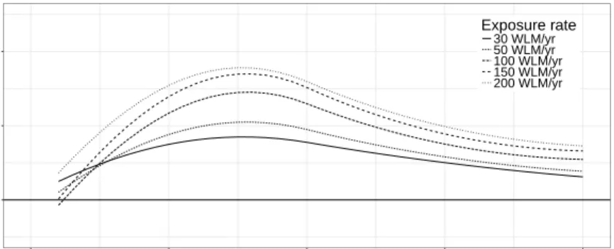
150 WLM/yr 200 WLM/yr 50 WLM/yr 100 WLM/yr 0 10 20 30 40 0 10 20 30 40 1.0 1.1 1.2 1.0 1.1 1.2 Lag (yr) HR Silica with Silica dust without Silica dust
Model constant
piece−wise constant
Fig. A1 Comparison of lag-response curves for the hazard ratio (HR) of DLMs L1 to L4 for four different radon exposure rates 50 WLM/yr, 100 WLM/yr, 150 WLM/yr and 200 WLM/yr, in models L2 and L4 (red lines) silica dust is a confounder but not in models L1 and L3 (blue lines), for models L1 and L2 (solid lines) the lag-response is constant, for models L3 and L4 (dashed lines) the lag-response is piecewise constant with cut-off points at 10 yr, 20 yr and 30 yr.
1 2 3 4 5 6 7 8 9 10 11 12 13 14 15 16 17 18 19 20 21 22 23 24 25 26 27 28 29 30 31 32 33 34 35 36 37 38 39 40 41 42 43 44 45 46 47 48 49 50
Table A1 Properties and goodness-of-fit for DLMs L1 to L5 with a linear exposure response
f(xt−`) to annual radon exposure rates and varying shapes of lag responses wx(`), for
piecewise constant lag response cut-offs are located 10 yr, 20 yr and 30 yr,dfdenotes the number of model parameters, lowest values for AIC and BIC in bold, L5 is the preferred DLM.
The last column contains the p-values of LRTs where L2 and L3 are tested against L1 and L4 is tested against L2. All p-values are smaller than 0.05 which indicates a superior goodness-of-fit for more complex models and models controlling for silica dust. Model L5 can not be tested via LRT as it is not nested.
Model wx(`) AIC BIC df silica dust p
L1 constant 58427.86 58445.87 3 no –
L2 constant 58353.14 58389.17 6 yes <0.01
L3 piecewise constant 58404.23 58440.26 6 no <0.01 L4 piecewise constant 58350.07 58404.11 9 yes 0.028 L5 B-Spline (degree 2, 1 knot)1 58345.58 58393.62 8 yes – 1minimum lag`
0set to 2 yr
The next phase of model development was concerned with improvements of the lag responsewx(`) of DLMs. To determine the shape ofwx(`) we tested models with B-Splines
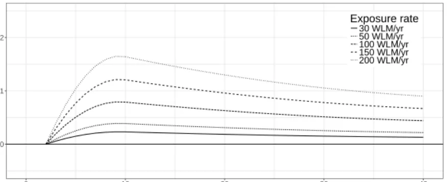
of degrees one to six with zero up to five knots on equally spaced quantiles of the weighted lag distribution. The intercept of the hazard ratio (HR) on the y-axis was determined in the fits. For most of the curves the intercepting HR was estimated<1, and the HR exceeded 1 only after a lag of three years. This observation strengthens the argument that no risk occurs in the early years after exposure. In our models we set the minimum lag to 2 yr. However, we do not allow hormetic effects in the lag response and fix HRs smaller than one at early lags to zero. For the preferred DLM L5 the shape of the lag response is shown in Fig. A2 for various radon exposure rates. Modeled with a quadratic B-spline and one knot, lag 1 2 3 4 5 6 7 8 9 10 11 12 13 14 15 16 17 18 19 20 21 22 23 24 25 26 27 28 29 30 31 32 33 34 35 36 37 38 39 40 41 42 43 44 45 46 47 48 49 50
response curves for model L5 exhibit a maximum at about 9 yr after first exposure followed by a steady decline. Properties of model L5 are given in Table A1.
1.0 1.1 1.2 0 10 20 30 40 Lag (yr) HR Exposure rate 30 WLM/yr 50 WLM/yr 100 WLM/yr 150 WLM/yr 200 WLM/yr
Fig. A2 Lag-response curves for the hazard ratio (HR) of the preferred DLM L5 for five radon exposure rates between 30 WLM/yr and 200 WLM/yr.
1 2 3 4 5 6 7 8 9 10 11 12 13 14 15 16 17 18 19 20 21 22 23 24 25 26 27 28 29 30 31 32 33 34 35 36 37 38 39 40 41 42 43 44 45 46 47 48 49 50
A.2 DLNM NL3 with right-constrained lag response at 40 yr
1.0 1.1 1.2
0 10 20 30 40
Time since exposure (yr)
HR Exposure rate 30 WLM/yr 50 WLM/yr 100 WLM/yr 150 WLM/yr 200 WLM/yr 1.0 1.1 1.2 0 100 200 300
Exposure rate (WLM/yr)
Time since exposure
10 yr 15 yr 20 yr30 yr
Fig. A3 Selected lag response curves of the hazard ratio (HR) for exposure rates between 30 WLM/yr and 200 WLM/yr (left panel) and exposure response curves for time since exposure between 10 yr and 30 yr (right panel) for DLNM NL3 with right-constrained lag response function at 40 yr.
1 2 3 4 5 6 7 8 9 10 11 12 13 14 15 16 17 18 19 20 21 22 23 24 25 26 27 28 29 30 31 32 33 34 35 36 37 38 39 40 41 42 43 44 45 46 47 48 49 50
Exposure r ate (WLM/yr) 0 50 100 150 200 250 300 Time since e xposure (yr) 5 10 15 20 25 30 35 40 HR 0.90 0.95 1.00 1.05 1.10 1.15 1.20 1.25
Fig. A4 The exposure-lag response surface for the hazard ratio (HR) of DLNM NL3 with right-constrained lag response function at 40 yr.
1 2 3 4 5 6 7 8 9 10 11 12 13 14 15 16 17 18 19 20 21 22 23 24 25 26 27 28 29 30 31 32 33 34 35 36 37 38 39 40 41 42 43 44 45 46 47 48 49 50
A.3 Estimates for confounders age at begin of employment, calendar year and silica dust exposure for the preferred DLNM NL4
1.0 1.1 1.2
0 10 20 30 40
Time since exposure (yr)
HR
Exposure rate (silica)
5 mg/m3/yr 4 mg/m3/yr 3 mg/m3/yr 2 mg/m3/yr 1 mg/m3/yr 1.0 1.1 1.2 0 1 2 3 4 5
Exposure rate (silica)
Time since exposure
10 yr 20 yr 30 yr
Fig. A5 Selected lag response curves of the hazard ratio (HR) for exposure rates between 1 mg/myr 3 and 5 mg/myr 3 (left panel) and exposure response curves for time since exposure between 10 yr and 30 yr (right panel) for silica dust for the preferred DLNM NL4.
Table A2 Estimates ofcalandabefrom DLNM NL4
β exp(β) σβ p-value cal -0.0101 0.9900 0.0044 0.0233 abe -0.0231 0.9772 0.0048 0.0000 1 2 3 4 5 6 7 8 9 10 11 12 13 14 15 16 17 18 19 20 21 22 23 24 25 26 27 28 29 30 31 32 33 34 35 36 37 38 39 40 41 42 43 44 45 46 47 48 49 50
Table A3 Estimates of cross-basis coefficients for the preferred DLNM NL4 ηx,[i,j] exp(ηx,[i,j]) σηx,[i,j] p-value
B1Exp·B1lag -0.0587 0.9430 0.0184 0.0014 B1Exp·B2lag 0.0835 1.0871 0.0250 0.0008 B1Exp·B3lag -0.1075 0.8980 0.0381 0.0047 B2Exp·B1lag 0.0691 1.0715 0.0241 0.0041 B2Exp·B2lag 0.0456 1.0466 0.0241 0.0590 B2Exp·B3lag 0.0176 1.0177 0.0251 0.4841 B3Exp·B1lag 0.3600 1.4333 0.0988 0.0003 B3Exp·B2lag 0.0698 1.0723 0.0824 0.3970 B3Exp·B3lag 0.0997 1.1048 0.0756 0.1875 B4Exp·B1lag 0.1133 1.1199 0.1128 0.3154 B4Exp·B2lag 0.0901 1.0942 0.1022 0.3784 B4Exp·B3lag 0.0718 1.0744 0.1001 0.4731 1 2 3 4 5 6 7 8 9 10 11 12 13 14 15 16 17 18 19 20 21 22 23 24 25 26 27 28 29 30 31 32 33 34 35 36 37 38 39 40 41 42 43 44 45 46 47 48 49 50