This is the author’s version of a work that was submitted/accepted for pub-lication in the following source:
Vo, Brenda N.,Drovandi, Christopher C., &Pettitt, Anthony N. (2015)
Bayesian parametric bootstrap for models with intractable likelihoods. [Working Paper]
(Unpublished)
This file was downloaded from: http://eprints.qut.edu.au/86986/
c
Copyright 2015 QUT & the Authors
Notice: Changes introduced as a result of publishing processes such as copy-editing and formatting may not be reflected in this document. For a definitive version of this work, please refer to the published source:
Bayesian parametric bootstrap for models with
intractable likelihoods
Brenda N Vo1,2,*, Christopher C Drovandi1,2, and Anthony N Pettitt1,2
1School of Mathematical Sciences, Queensland University of Technology (QUT), Brisbane, Australia. 2ARC Centre of Excellence for Mathematical & Statistical Frontiers (ACEMS), QUT, Brisbane, Australia. *Corresponding author
*Email: [email protected]
Abstract
In this paper it is demonstrated how the Bayesian parametric bootstrap can be adapted to models with intractable likelihoods. The approach is most appealing when the semi-automatic approx-imate Bayesian computation (ABC) summary statistics are selected. After a pilot run of ABC, the likelihood-free parametric bootstrap approach requires very few model simulations to produce an approximate posterior, which can be a useful approximation in its own right. An alternative is to use this approximation as a proposal distribution in ABC algorithms to make them more efficient. In this paper, the parametric bootstrap approximation is used to form the initial import-ance distribution for the sequential Monte Carlo and the ABC importimport-ance and rejection sampling algorithms. The new approach is illustrated through a simulation study of the univariate g-and-k quantile distribution, and is used to infer parameter values of a stochastic model describing expanding melanoma cell colonies.
1 Introduction
In the Bayesian framework, the objective is to obtain the posterior distribution of the model para-meters, which is the distribution of the unknown parameters given the observed data. Computing these posterior distributions generally depend on the so-called likelihood function, the distribution of the data given parameter values. However, for many complex models in biological, medical and ecological sciences, the likelihood functions are not available in an analytical form and are compu-tationally intractable. To overcome this limitation, approximate Bayesian computation (ABC), a class of Bayesian “likelihood-free” techniques, has emerged, which avoids direct evaluation of the likelihood through repeated simulation of data from the model. As such, ABC methods permit Bayesian inference for models with intractable likelihoods, when simulation from the model for a range of parameter values is feasible.
ABC methods have been successfully applied in a wide range of problems such as population genetics [1], infectious diseases [2, 3], astronomical model analysis [4] and cell biology [5, 6]. The first ABC algorithm, ABC rejection sampling, was pioneered by Pritchard et al. [7]. In this ABC algorithm, parameter values are often simulated from the prior distribution and are accepted if they produce simulated data, x, that are “close enough” to the observed data, y. That is the distance between the simulated and the observed data,ρ(x,y), is not greater than a tolerance . Although this algorithm is easy to implement and is embarrassingly parallel, its acceptance rate is low, especially for complex models where the prior distribution is substantially different from the posterior. To improve the computational efficiency, several methods were proposed including regression adjustment [1, 8], a Markov chain Monte Carlo approach to ABC (MCMC ABC) [9, 10] and a sequential Monte Carlo approach to ABC (SMC ABC) [5, 11–13].
The original SMC ABC algorithm was pioneered by Sission et al. [11] and later was developed by Beaumont et al. [14] and Sission et al. [15]. SMC ABC algorithms generally involve a sequential importance sampling technique. Instead of drawing a parameter value one at a time as in ABC rejection sampling, the SMC ABC algorithms work with a large set of parameter values simultan-eously and treats each parameter vector as a particle. A set of particles are often simulated from the prior distribution and are propagated at each stage of the algorithm by re-sampling, perturb-ing and re-weightperturb-ing techniques. Thus, this last class of ABC aims to draw proposed parameters in high posterior support regions, rather than the entire parameter space. In the literature, there
are several modified and extended versions of the original SMC ABC algorithm. For example, Drovandi & Pettitt [13] and De Moral et al. [16] proposed a technique to automatically determine the sequence of tolerances, Bonassi & West [17] suggested a new weighting scheme that takes into account the closeness between the observed and the simulated data, and Vo et al. [5] proposed an adaptive SMC algorithm that overcomes the problem of particle duplication in [13]. However, all of these algorithms often start from the prior, which can be inefficient and require a large number of model simulations to obtain a reasonable approximation to the posterior distribution.
It has been shown that, for some cases, bootstrap methods are useful for numerical calculation of Bayes posterior distributions [18–20]. In particular, Efron [19] proposed the use of parametric bootstrap and a re-weighting scheme to approximate posterior distributions and its expectations. This approach is efficient and computationally straightforward. However, it depends upon an analytical expression for the sampling density of a statistic and a point estimate of the parameter, which is intractable for a model with an intractable likelihood. We show in this article that nevertheless parametric bootstrap samples can provide useful approximations to the posterior in the context of ABC.
This paper has two main innovations. The first innovation is the combination of the Bayesian bootstrap [19] and the semi-automatic approach to ABC [21], which uses regressions to estimate the posterior means of the model parameters based on the initial set of summary statistics. After a pilot run of ABC, the likelihood-free parametric bootstrap approach can be performed using the point estimate obtained from fitting a regression [21]. This parametric bootstrap (PB) distribution requires very few model simulations to produce an approximate posterior, which can be a useful approximation in its own right. The second innovation is to integrate the PB approximation above with ABC algorithms. In this paper, the PB distributions are used as an initial importance distribution for SMC ABC algorithms and ABC importance and rejection sampling (ABC IS). Hereafter, we refer to these new algorithms as PB SMC ABC and PB ABC IS algorithms, respectively.
We apply the methodology to a simulated data set from the g-and-k quantile distribution of [22] as a test example to validate the approach. Using this simulated dataset, we also compare the performance of several ABC algorithms: PB SMC ABC, PB ABC IS and the SMC ABC algorithm proposed in [5]. We then apply the new collection of methods to a discrete stochastic model
(agent-based model) [5] that describes the expansion of human melanoma cell colonies. The model is a random walk model that incorporates cell motility, cell proliferation and cell-to-cell adhesion in a barrier assay. The observed data are the image-based data that show the entire population of cells after a specific experimental time period. Simulations of cell experiments from the discrete model is highly computationally intensive, especially for a large cell proliferation rate. Thus, it requires an ABC algorithm that is efficient in terms of the number of model simulations.
This article is organized as follows. ABC importance and rejection sampling, and SMC ABC are briefly reviewed in Section 2. The Bayesian parametric bootstrap [19] is described in Section 3. We demonstrate how the Bayesian parametric boostrap can be efficiently adapted to likelihood-free problems using the semi-automatic ABC summary statistics [21] and how to use this result to derive the initial distribution for ABC algorithms in Section 4. Section 5 contains the results from a simulation study using the g-and-k quantile distribution and comparing performance of various ABC algorithms. In Section 6, we apply our new algorithms to the experimental data of human malignant melanoma cells (MM127) [5, 23] in a barrier assay. The article is concluded with a discussion in Section 7.
2 Approximate Bayesian computation
Letθ, θ ∈ Θ, be the parameter of a model with an intractable likelihood,p(y|θ), where y is the observed data. Assuming a prior distribution of θ given by p(θ), ABC is a well-known statistical inferential approach to approximate the posteriorp(θ|y)∝p(θ)p(y|θ) when the likelihood function is not available in an analytical form and is not computationally tractable.
ABC algorithms generally consist of three major steps: sampling a proposed parameter θ?, sim-ulating data x as per the observed data structure from the model p(·|θ?) and comparing x with the observed datay. Different ABC algorithms are distinguished by the process of sampling pro-posed parameters. In ABC, direct comparison between the observed and the simulated datasets is often inefficient (or impossible), especially when the data is high dimensional [24]. Thus, we consider a vector of summary statistics s(·) = {s1(·), . . . , sd(·)}, which have smaller dimension than the full data. For simplicity, we denotesobs =s(y) ands=s(x). To measure the closeness betweenx and y, via the closeness between s and sobs, we use a distance metric ρ(s,sobs) and a kernel weighting function K(ρ(s,sobs)), where >0 is a bandwidth and referred to as the ABC
tolerance.
ABC typically makes two approximations. The first approximation relates to the choice of sum-mary statistics s(·). The posterior p(θ|y) is approximated by p(θ|sobs). If s(·) is sufficient for θ then no information is lost and p(θ|sobs) =p(θ|y). However, low dimensional sufficient statistics are generally not available for models with an intractable likelihood. Therefore, the choice of summary statistics is crucial to control the first source of ABC error. The second approximation is due to the ABC tolerance. The ABC posterior is constructed as
pABC,(θ|sobs)∝p(θ)p(sobs|θ), (1)
with
p(sobs|θ) =
Z
K(ρ(sobs,s))p(s|θ)ds. (2)
In practice, the kernel weighting function K(ρ(sobs,s)) is often chosen as an indicator function, 1{ρ(sobs,s)≤}, that is unity if the condition involving the discrepancy is satisfied. Approximating the target p(θ|sobs) by pABC,(θ|sobs) can be shown to be a good approximation if is small enough [24]. The choice of represents a trade-off between accuracy and computational effort. The smallerleads to the more accurate approximation in Eq. 2 but more variable weights which are proportional toK(ρ(sobs,s)) if a simple ABC IS algorithm is applied. Thus, a large amount of proposed parameters will be needed for an adequate approximation with a reasonable effective sample size. To improve the computational efficiency, Beaumont et al. [1] proposed a regression adjustment approach by regressing the values of the parameters of the ABC posterior against the corresponding simulated summary statistics. Other improvements focus on developing more efficient ABC algorithms using MCMC sampling [9, 10] or SMC sampling [5, 11–13].
Our suggestion is that the efficiency of ABC algorithms can be improved if there is a good analytical approximation to the posterior p(θ|sobs) that can be obtained quickly. For example, such an approximation can be used to form importance distributions for ABC IS or SMC ABC algorithms. In Section 3, we describe an adaptation of the Bayesian parametric bootstrap that can be used to form this initial approximation. The remainder of this section briefly discusses the ABC IS algorithm [21] and a current SMC ABC algorithm described in Vo et al. [5].
2.1 ABC importance and rejection sampling
Fearnhead & Prangle [21] provide an importance and rejection sampling implementation of ABC for which the output is a weighted sample of values from the ABC posterior distribution (Ap-pendix, Algorithm 1). For simplicity, we set up the acceptance-rejection step (line 6) using the indicator function 1{ρ(sobs,s)≤}.
In this algorithm, a proposed parameterθ? is drawn from an importance distribution, g(θ). Each proposed value θ? is assigned a weight proportional to p(θ?)/g(θ?) if it produces simulated data that satisfies the discrepancy condition, otherwise its weight is zero. When g(θ) = p(θ), this algorithm becomes ABC rejection sampling which is similar to the algorithm of Beaumont et al. [1].
The advantage of this algorithm is that it generates independent samples and the algorithm can easily be run in parallel. However, if a good importance distribution is not available and the prior distribution is substantially different from the posterior, this algorithm results in low acceptance rates and thus, is computationally inefficient.
2.2 SMC ABC
In this paper, we use the SMC ABC algorithm of Vo et al. [5], which was shown to have improve-ments over the algorithms of Sisson et al. [15], Beaumont et al. [14] and Drovandi & Pettitt [13] for an application in cell biology. For a non-increasing sequence of tolerances {t}Tt=1, the SMC
ABC algorithm aims to obtain a set ofN weighted particles from the following sequence of targets
pABC,t(θ,s|sobs)∝p(θ)p(s|θ)1{ρ(s,sobs)≤t}.
In brief, the SMC ABC algorithm of Vo et al. [5] integrates the advantages of automatically determining tolerance values from [13,16] and the advantage of geometric sampling from a proposal distribution until an acceptable parameter value is obtained [14, 15]. Pseudo code for this SMC ABC algorithm is provided in the Appendix, Algorithm 2. In this SMC ABC algorithm, the only tuning parameter isα∈[0,1] which is the proportion of particles to keep at each iteration among the N particles. The stopping criterion is either the minimal acceptance rate, paccmin, or a target
tolerance, T.
For many applications of ABC, the most computationally intensive procedure is the model sim-ulation process. Therefore, we aim to develop an efficient ABC algorithm that can achieve a low tolerance value within a manageable number of model simulations. To achieve this, we incorpor-ate an importance distribution at the initial iteration,t = 0, of the SMC ABC algorithm. Section 3 will describe how to obtain such an importance distribution while the detail of the algorithms will be provided in Section 4.
2.3 Summary statistics
In applications of ABC, we aim to choose a vector of summary statistics that has low dimension and is close to sufficient to avoid the loss of information. In the literature, various approaches have been proposed to choose useful summary statistics including a sequential scheme based on the principle of approximate sufficiency [25], partial least-squares regression [26], indirect inference [27] and machine learning methods [28]. In this paper, we implement the method proposed by Fearnhead & Prangle [21] who use the estimates of the posterior means of θ as the summary statistics. These posterior means are obtained via regression. We note that the rational for ABC is to obtain an approximation to the posterior distribution p(θ|sobs) not just a point estimate.
Initially,M draws of{θi}Mi=1 are made from the prior distribution. If the priorp(θ) is diffuse then
draws ofθi can be restricted to regions of non-negligible posterior density found using a pilot run of ABC. Each parameter θi is then used to simulate a dataset xi from the model, xi ∼ p(·|θi), i= 1, . . . , M.
We denotesinitas the summary statistics for the pilot run,sreg as the summary statistics that are used in the regression procedure and sF P as the derived summary statistics from the regression procedure which are used in the final ABC runs. We fit the model
θi =α+βTf(xi) +i, i= 1, . . . , M, (3)
data is not feasible). Different choices of f(·) could be considered to obtain a better fit in the regression. Various possible regression models can be fitted and compared using standard data analytic regression diagnostic and model choice methods. In this paper, to find the best regression model, we employ a stepwise (bidirectional) regression method and the Bayesian information criterion (BIC) for model selection.
The expected value ofθi given the simulated summary statisticssregi ,E[θi|sregi ], is then estimated by ˆα+ ˆβTf sreg
i
, i = 1, . . . , M, where the intercept parameter ˆα and the vector of regression coefficients ˆβ is estimated from the best regression model. The derived summary statistic sF P is then interpreted as the estimated posterior mean ofθ obtain from the regression procedure. Thus, using this dimension reduction approach, we have only one summary statistic per parameter. In practice, if the parameter θ is vector valued, then a multiple linear regression model (Eq. 3) is fitted to each component ofθin turn, with possibly a different functionf(·) and different estimates of ˆα and ˆβ.
2.4 Discrepancy function
We note that the derived summary statistics can have different scales and correlations between summaries. Thus, we consider the Mahalanobis distance to compare the summary statistics of the observed and the simulated data,sF P
obs and sF P. This discrepancy function is given by
ρ(y,x) = sF Pobs −sF PT ×W−1× sF Pobs −sF P,
whereW is an estimate of the covariance matrix of the summary statisticssF P. To estimateW, we generate 100 simulated datasets{xi|θˆ}i100=1, using the estimated posterior mean ˆθ = sF Pobs, obtained from the regression step above. For each simulated datasetxi, we compute the summary statistics sregi , then obtain the derived vector of summary statistics sF Pi . W is subsequently estimated by cov {sF Pi }100
i=1
.
3 Bayesian parametric bootstrap
The Bayesian parametric bootstrap [19] is introduced here. In this section, the summary statistics
of θ, ˆθ, as a function ofsobs. For simplicity we denote ˆθ=sobs.
The bootstrap independently generatesB values of the statisticsj =s(xj),j = 1, . . . , B wherexj is a simulated data set from the modelp(·|θˆ). Each sample estimate ofθ,θj =sj,j = 1, . . . , B, is a parametric bootstrap replication of ˆθ. By re-weighting these points with an importance weight
wj =
[p(θ)]θ=sj[p(s|θ)]s=sobs,θ=sj [p(s|θ)]s=sj,θ=sobs
, (4)
we obtain an estimated posterior distribution of θ given ˆθ. If the likelihood function of the summary statistics p(s|θ) can be evaluated then the importance weights (Eq. 4) can be found. However, for models with intractable likelihoods,p(s|θ) cannot be evaluated.
We consider a special case where the weights in Eq. (4) can be simplified. If the likelihood for s
is symmetric ins−θ (s and θ must be the same dimension), there exists a symmetric density h such thath(x) =h(−x) for allx. Denotep(s|θ) =h(s−θ), then the bootstrap provides values of
[p(s|θ)]s=sj,θ=sobs = [h(s−θ)]s=sj,θ=sobs = [h(θ−s)]s=sj,θ=sobs = [p(s|θ)]s=sobs,θ=sj,
(5)
for j = 1, . . . , B. Therefore, the importance weights for the posterior in Eq. 4 become just the prior evaluated at the bootstrap replication sj
wj ∝[p(θ)]θ=sj, j = 1, . . . , B. (6)
In general, of course, without the assumption of exact symmetry, the bootstrap sample gives an approximation to the likelihood [p(s|θ)]s=sobs,θ=sj,j = 1, . . . , B. The weighted samples{θj, wj}
B
j=1
derived from Eq. (6), where θj = sj, j = 1, . . . , B, gives an approximation to the posterior, p(θ|sobs).
4 Coupling Bayesian parametric bootstrap with ABC
This section proposes the two innovations: (i) how to obtain the PB distribution for models with intractable likelihoods and (ii) how to incorporate this PB distribution in ABC algorithms to
improve efficiency.
4.1 PB approximation for models with intractable likelihoods
To apply the Bayesian parametric bootstrap idea for models with intractable likelihoods, it is computationally too intensive to take ˆθ as a point estimate of the ABC posterior pABC,(θ|sobs) obtained from the ABC algorithms above. What is required is a computationally cheap likelihood-free Bayesian estimator. Thus, the main idea here is to perform Bayesian parametric bootstrap with ˆθ obtained from the semi-automatic approach [21]. Fearnhead & Prangle [21] interpret the ˆ
θ as an estimate of the posterior mean, but we note that the prior density does not factor into the regression analysis performed in Eq.3. Here we interpret ˆθ simply as a cheap likelihood-free estimator.
Sampling simulated data x for ABC requires different values of θ while obtaining the Bayesian bootstrap only requires sampling x for fixed ˆθ = ˆα + ˆβTf
j(y) obtained from the regression approach in Section 2.3. Assuming that the likelihood for the summary statistic p(s|θ) has the symmetry property so that the following holds
[p(s|θ)]s=sj,θ=sobs = [p(s|θ)]s=sobs,θ=sj, (7)
then the weighted samples {θj, wj}Bj=1 gives an approximation to the posterior p(θ|sobs). Here θj = sj and the importance weights wj are given by the prior (Eq. 6). This approximation is extremely computationally efficient having used only (Npilot+M+B) simulations from the model p(·|θ). Here, Npilot is the number of model simulations from the ABC pilot run. Pseudo code to perform the Bayesian parametric bootstrap in this section is provided in Appendix, Algorithm 3.
4.2 PB approximation in ABC
If the analyst believes that the symmetry property approximation is poor then the ABC Bayesian bootstrap approximation {θj, wj}Bj=1 can be used to form an analytic approximation to the
pos-terior p(θ|sobs) which we denote by g(θ). The analytical approximation can be taken as a para-metric distribution such as a multivariate normal or a kernel density estimate. The approximation g(θ) can be used as a proposal density in the ABC IS algorithm [21] (see Appendix, Algorithm
1) or an initial importance distribution for the SMC ABC algorithm (see Appendix, Algorithm 4), and we discuss other options in Section 7.
4.2.1 Setting the tolerance
We can investigate the ABC IS algorithm (Appendix, Algorithm 1) when the importance distri-bution is a good approximation to the posteriorp(θ|sobs). In this algorithm we wish to investigate the probability of acceptanceK{(s−sobs)/}in Step 6 whenθ in Step 4 is simulated with density g(θ) equal to a good approximation to the posteriorp(θ|sobs). Here max{K(x)}= 1. The expec-ted value of the probability of acceptance, pacc, is a measure of the computational efficiency of the importance distribution. This depends on the choice of , the larger the value of , the larger the expected value of the probability of acceptance.
For illustration, we takeK(x) proportional to the standard Gaussian density so thatK(x) ∝ e−x 2 2 .
We assume that the likelihoodp(s|θ) is Gaussian with meanθ and variance v, denotedN(s;θ, v), and the priorp(θ) is approximately uniform so that the posteriorp(θ|sobs) is GaussianN(θ;sobs, v). From equations 1 and 2, the marginalpABC,(θ|sobs) is given by
pABC,(θ|sobs)∝p(θ)
Z
K{(s−sobs)/}p(s|θ)ds
∝N(θ;sobs, v+2).
(8)
We note that K{(s−sobs)/} and p(s|θ) are proportional and equal, respectively, to Gaussian densities fors. Thus, comparingpABC,(θ|sobs) with p(θ|sobs), the variance of the ABC posterior is inflated by2, the inaccuracy of ABC.
To find the expected value of the probability of acceptance we need the posterior predictive distribution for ˜s which is generated by ˜s|θ ∼ p(˜s|θ), with θ ∼ p(θ|sobs). Marginalizing over θ we obtain ˜s|sobs ∼N(sobs,2v).
The expected probability of acceptance,pacc, is given by
pacc =
Z
which simplifies to
Z
e−t 2
22N(t; 0,2v)dt,
putting t = ˜s−sobs. We obtain the expected probability of acceptance pacc = √2v+2. Given
that the ABC posterior has variance v +2 inflated by 2 over the true posterior variance v, a reasonable choice for is a small fraction of √v,k√v. So =k√v gives pacc = √2+kk2.
If k = 0.1 and = 0.1√v then pacc = 0.071, which demonstrates the unusual computational demands of ABC. That is, in order to obtain a reasonably accurate ABC posterior approximation, with 1% increase of the posterior variance, the expected probability of the ABC acceptance step, Step 3 in Algorithm 1, is small, 0.07, even when it is possible to sample from an accurate approximation of the posterior.
If the requirement is anN particle ABC approximation{θj, wj}Nj=1 using the Bayesian bootstrap
and Algorithm 1 using = 0.1√v then the expected total required number of simulations from the likelihood isM +B+N/pacc or M +B+ 14.2N.
We note that if θ in Step 1 of the importance and rejection sampling ABC algorithm is simu-lated from densityg(θ) which is taken as the Bayesian bootstrap approximation with an inflated variance, that is N(sobs, Kv), we have ˜s|sobs ∼ N(sobs,(K + 1)v). Then, pacc is computed by pacc = √ k
(K+1)+k2.
We note pacc decreases as O(K− 1
2). Typically we would take K = 2 or larger in the importance
densityg(θ) in order to have thicker tails for the importance density than the target density. If, on the other hand, we used a very diffuse importance density with largeK thenpacc ≈ √kK. Withk = 0.1 as above andK = 1002 this givespacc= 10−3. Thus, the ABC IS algorithm with these settings would requireM+1000N simulations from the likelihood, roughly 70 times more simulations from the likelihood than the version above using the Bayesian bootstrap approximation.
5 Test example
5.1 Model and data
We now validate our new collection of methods using synthetically generated data from the g-and-k quantile distribution [22]. The g-g-and-k-distribution is a class of quantile distributions and
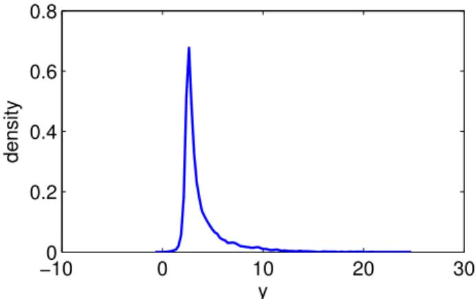
−100 0 10 20 30 0.2 0.4 0.6 0.8 y density
Fig. 1: Estimated probability density based on the simulated dataset from the g-and-k distribution.
it is defined by its quantile function, the inverse cumulative distribution function
Q(z(u);θ) =F−1(z(u);θ) =a+b 1 +c1−exp(−gz(u)) 1 + exp(−gz(u)) 1 +z(u)2kz(u), (9)
where z(u) is the u-quantile of the standard normal distribution and θ = (a, b, c, g, k) is the unknown parameter. Given a fixed value of c, c = 0.8 [22], the g-and-k distribution consists of four unknown parameters,a, b, gandk, which are related to location, scale, skewness and kurtosis, respectively. Here, the likelihood function can be evaluated numerically [22], so we can compare ABC posterior distributions with the distribution of the samples that are drawn from the true posteriors.
Firstly, we consider a simulated dataset that consists of n = 104 independent draws from the
g-and-k distribution with parameters θ = (a, b, g, k) = (3,1,2,0.5). A uniform prior (0,10)4 is
used for the parameters. This is similar to the example used in [21,29,30]. A plot of the estimated probability density function based on this dataset is shown in Fig. 1. The data shows significant skew and kurtosis.
5.2 Results
For the ABC pilot run, we consider sinit as the set of octiles [30], and the Euclidean distance between summary statistics. In this pilot run, we use the SMC ABC algorithm of Vo et al. [5] and set N = 1,000. After 18 iterations, we find that the training regions for a, b, g and k are given by (2.8, 3.2), (0.7, 1.3), (1, 4) and (0, 1), respectively. The number of model simulations for the pilot run is 25,012 and the probability of acceptance in the last iteration is approximately 27%.
For the regression procedure, we simulate M = 5,000 datasets from the parameters that are drawn from the training regions above. We consider sreg = {L
i}19i=1, where Li, i = 1, . . . ,19 is the (0.05×i)th quantile. A bidirectional stepwise regression is then fitted to determine a 4-dimensional summary statistic sF P. A point estimate of ˆθ obtained from the regression is ˆ
θ= (ˆa,ˆb,g,ˆ kˆ) = (2.9970,1.0064,2.0426,0.4965).
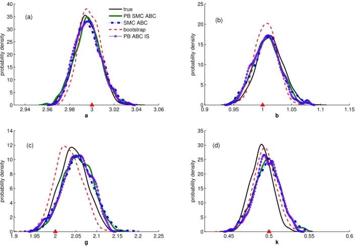
Using this value of ˆθ, we perform the Bayesian parametric bootstrap with B = 1,000 (see Ap-pendix, Algorithm 3). To incorporate the Bayesian parametric bootstrap samples into ABC algorithms, we propose to use a multivariate normal approximation, which appears to be reason-ably close to the Bayesian parametric distribution. We fit a multivariate normal distribution to the PB samples and use it as an initial importance distribution,g(θ), in the new algorithms: PB SMC ABC and PB ABC IS. In order to help ensure coverage of the tails, the covariance matrix of g(θ) is set as twice the empirical covariance matrix based on the PB samples. The ABC posterior distributions ofa, b, g andk from the new PB ABC algorithms are plotted in Fig. 2 together with the results from using the SMC ABC algorithm of Vo et al. [5].
Since the regression procedure was performed for a training region rather than the entire parameter space, computing summary statistics for simulated data with parameters that are drawn from outside these regions can lead to extrapolation, which was addressed in Fearnhead & Prangle [21] by using MCMC to ensure that most of proposals are made within the training region. To address the extrapolation issue within SMC ABC, we form an initial importance distribution from the pilot run. For this example, we use a multivariate normal distribution with covariance matrix esimated from the pilot run samples inflated by a factor of two.
Figure 2 shows a comparison between the results using the true likelihood (solid black), the PB distribution (dashed red), and the ABC posteriors results from three different ABC algorithms: PB SMC ABC (solid green), SMC ABC [5] (solid blue) and PB ABC IS (circle purple). The exact MCMC algorithm, using the true likelihood of the g-and-k distribution, was run for 20,000 iterations, with a thinning interval of 10 to obtain accurate estimates of the true posteriors (see [22, 31]). It can be seen that the PB distribution provides a good approximation to the true posteriors for alla, b, g and k, given a very small number, 31,012, model simulations.
For the PB SMC ABC algorithm, we use the summary statistics sF P and a probability of ac-ceptance, pacc, of 0.4% to achieve a tolerance = 0.78. This ABC run requires 577,015 model
2.94 2.96 2.98 3 3.02 3.04 3.06 0 5 10 15 20 25 30 35 40 a probability density (a) true PB SMC ABC SMC ABC bootstrap PB ABC IS 0.9 0.95 1 1.05 1.1 1.15 0 5 10 15 20 25 b probability density (b) 1.9 1.95 2 2.05 2.1 2.15 2.2 2.25 0 2 4 6 8 10 12 14 g probability density (c) 0.45 0.5 0.55 0.6 0 5 10 15 20 25 30 35 k probability density (d)
Fig. 2: Posterior distributions for the parameters of the g-and-k simulated dataset. In all subfigures, results from using the true likelihood (solid black), the Bayesian parameteric bootstrap (dashed red), the PB SMC ABC (solid green), the plain SMC ABC (dashed dotted blue) and the PB ABC IS (circle purple) are shown. The true values
ofa, b, gandkare plotted as red upper triangles.
simulations forN = 2,000 particles. The effective sample size, ESS, is approximately 1,413. The ABC posterior distributions for all parameters are well-defined and are very close to the true posteriors. In particular, the results for a and b are very accurate, suggesting that the summary statisticssF P are close to sufficient for these parameters. The results for g and k obtained from the PB SMC ABC show slight deviation from the true posteriors and also a small loss of precision. The SMC ABC algorithm of Vo et al. [5] was run using the same values for N, and the same summary statisticssF P as in PB SMC ABC. This algorithm produces an ESS of 1,390 and thep
acc of 0.4%. For all four parameters, the posteriors resulting from the plain SMC ABC and the PB SMC ABC are quite similar, as expected. However, the PB SMC ABC starts from the importance distribution g(θ) which is very close to the posteriors, whereas the plain SMC ABC starts from an importance distribution formed from the pilot run. Thus, the PB SMC ABC requires fewer number of model simulations, about 100,000 simulations less than the SMC ABC algorithm. Given the same amount of computational effort (in terms of the number of model simulations)
and the target tolerance, the PB ABC IS shows a slightly better probability of acceptance, 0.47%, resulting in 2,691 particles being kept. Even though the number of accepted particles for the PB ABC IS is higher than the PB SMC ABC, its ESS (1,103) is lower than the ESS from the PB SMC ABC. However, the samples from PB ABC IS are guaranteed to be statistically independent.
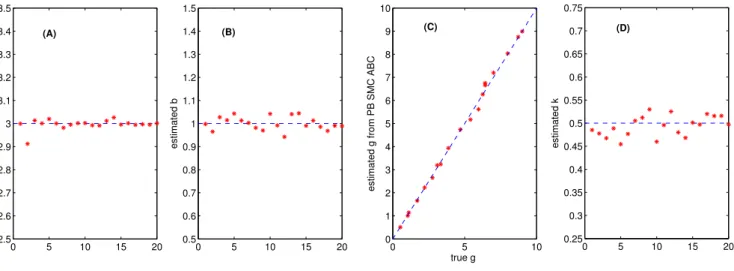
5.3 Results for different set of parameters
In this section, we aim to test our methodology for different set of parameters. Out of the four parameters, g is the hardest to obtain accurate Bayesian inferences for. So we keep the same a = 3, b = 1 and k = 0.5, and vary the value of g within (0, 10). We implement the PB SMC ABC on 20 simulated datasets of sizen= 104 that are drawn for 20 different values ofg. The PB
SMC ABC mean estimates of g are plotted against the true values of g in Fig. 3. Results from Fig. 3(C) for g suggest that posterior mean estimates from the PB SMC ABC are very close to the true values in all cases.
0 5 10 15 20 2.5 2.6 2.7 2.8 2.9 3 3.1 3.2 3.3 3.4 3.5 estimated a (A) 0 5 10 15 20 0.5 0.6 0.7 0.8 0.9 1 1.1 1.2 1.3 1.4 1.5 estimated b (B) 0 5 10 0 1 2 3 4 5 6 7 8 9 10 true g
estimated g from PB SMC ABC
(C) 0 5 10 15 20 0.25 0.3 0.35 0.4 0.45 0.5 0.55 0.6 0.65 0.7 0.75 estimated k (D)
Fig. 3: A comparison of the estimates from PB SMC ABC versus the true values ofa, b,gandkfor 20 simulated data sets.
6 Application to a collective cell spreading model
We now present our main application involving a discrete stochastic model describing the ex-pansion of melanoma cell populations [5]. Melanoma is a cancer that begins in the melanocytes and is the most dangerous form of skin cancer [32]. Melanoma is less common, approximately 5% of all skin cancer occurrences, but accounts for approximately 75% of skin cancer death [33].
The spatial expansion of melanoma cells is governed by various mechanisms including cell motil-ity, cell proliferation and cell-to-cell adhesion. Estimating these mechanisms can improve our understanding of melanoma biology and its response to treatment.
6.1 Data
We applied the new ABC algorithms to analyse an experiment of human malignant melanoma cells (MM127) [34, 35] in a circular barrier assay. Details of the experimental protocol were de-scribed in [23]. In brief, the experiment was conducted using a 24-well tissue culture plate, where each well has a diameter of 15.6 mm. Initially, 20,000 cells were evenly distributed within a metal-silicone barrier, of a diameter 6.0 mm, which was located in the centre of the well. The tissue culture plate was kept for one hour to allow the cells to attach to the surface. Subsequently, the barrier was lifted and the plate was incubated for two time durations of 24 or 48 hours. The experiment was repeated in triplicate. For each experiment, we obtained two types of images: (i) a population-scale image which shows the entire melanoma cell colony and (ii) individual-scale images which show the location of each cell in the population. For the application in this paper, we only analyse the experiments that were terminated at 24 hours. Details of the ABC analyses for experiments at 48 hours and experiments with different initial cell densities can be found in [5].
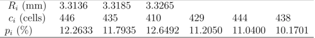
Initially, we summarise the experimental data using a high dimensional summary statistics,sinit, including three radii of the entire expanding melanoma colonies,{Ri}3i=1, the total number of cells,
{ci}6i=1, and the number of isolated cells, {pi}6i=1, in six subregions of the cell population. We
compute{Ri}3i=1 by locating the position of the leading edge, measuring the area of the spreading
cell population and converting this area into an equivalent circular radius. We average the{ci}6i=1
and{pi}6i=1over three replicates, to produce a total of 15 summary statistics. These processes were
performed using a segmentation algorithm written with the Matlab Image Processing Toolbox [5] and were repeated for images that were produced by the discrete model described in Section 6.2. For more details on the image analysis and how the summary statistics were obtained see [5]. Table 1 shows 15 observed summary statistics that is used for the ABC analysis in this section.
Table 1: Initial summary statistics for the experimental data. Results shown include three radii, {Ri}3i=1, the total number of cells, {ci}6i=1, and the number of isolated cells, {pi}6i=1,
in six subregions of the cell population (average over three replicates).
Ri (mm) 3.3136 3.3185 3.3265
ci (cells) 446 435 410 429 444 438
pi (%) 12.2633 11.7935 12.6492 11.2050 11.0400 10.1701
6.2 Model
To describe the spatial expansion of the melanoma cell population, we use a discrete stochastic model that incorporates cell motility, cell proliferation and cell-to-cell adhesion on a two-dimensional square lattice with spacing ∆. Each lattice site can be occupied by at most one cell. LetPm ∈[0,1] be the probability that an isolated agent will attempt to step a distance ∆ within a time step of duration τ, and Pp ∈[0,1] represent the probability that an agent will attempt to proliferate and deposit a daughter within a time step of durationτ. The strength of cell-to-cell adhesion is represented byq ∈[0,1].
To step from time t to time t+τ, C(t) agents are sampled, with replacement, and given the opportunity to move with probabilityPm×(1−q)n, where 0≤n≤4 is the number of occupied nearest neighbour sites. If an agent is at position (x, y) and has an opportunity to move, it will attempt to step to either (x±∆, y) or (x, y ±∆), with each target site chosen with equal probability. For increasing values ofq, neighbour agents adhere more tightly to each other and it is difficult for an agent to move away from its neighbours. A similar mechanism is employed for proliferation events. A proliferative agent at position (x, y) will attempt to deposit a daughter agent at (x±∆, y) or (x, y±∆), with each target site chosen with equal probability.
In this model, the cell motility rate is quantified in terms of the cell diffusivity,D,D = Pm∆2/4τ, and the cell proliferation rate,λ, is related byλ = Pp/τ [36]. A uniform priorU(0,1) is placed for all three parameters (Pm, q, Pp). For all model simulations, we use a time step duration τ as 0.04 h [5]. We apply ABC algorithms to obtain joint posterior distributions for (Pm, q, Pp), then use the values of ∆ andτ to rescale posterior distributions ofPm and Pp into posterior distributions of D and λ, respectively.
6.3 Parameter inferences
A pilot run was conducted using the SMC ABC algorithm of [5], incorporating all 15 summary statistics and using the Mahalanobis distance to compute the distance between the observed and the simulated summary statistics. We setN = 500 particles and a uniform prior (0,1) is placed on all the parametersPm, q andPp. Thepaccmin = 0.2 is used as a stopping criterion. We obtain the training regions for Pm, q and Pp as (0.07, 0.14), (0.14, 0.43) and (0.0010, 0.0018), respectively, using only 13,925 model simulations.
200 240 280 320 0 0.01 0.02 0.03 0.03 0.04 D (µm2h−1) probability density 0.2 0.25 0.3 0.35 0.4 0 2 4 6 8 10 12 14 16 q 0.030 0.035 0.04 0.045 50 100 150 200 250 300 350 λ (h−1) PB SMC ABC SMC ABC bootstrap
Fig. 4: ABC posterior distributions for D,q and λresulting from PB SMC ABC (solid red), SMC ABC of [5] (dashed black) and the Bayesian bootstrap distribution (dashed dotted blue).
Table 2: ABC posterior summary for D, q and λ for two different ABC algorithms
and the bootstrap distribution. Results shown include the posterior mean (and the 90% CI
in the parentheses) and the coefficient of variation, CV.
E[D] CV(D) E[q] CV(q) E[λ]×10−2 CV(λ)
(µm2h−1) (%) (%) (h−1) (%)
Bootstrap 250.1 (241.5, 277.7) 4.2 0.24 (0.20, 0.29) 10.5 3.77 (3.54, 4.01) 3.6
SMC ABC 234.6 (219.2, 248.1) 3.7 0.25 (0.21, 0.28) 9.2 3.73 (3.55, 3.94) 3.1
PB SMC ABC 234.0 (220.5, 248.0) 3.6 0.25 (0.21, 0.29) 9.1 3.73 (3.57, 3.92) 2.9
A regression analysis (Eq.3) was performed for each parameter in turn, usingM = 5,000 datasets that were generated by parameters in these training regions. We find that using f(sreg) =
sreg,{sreg}2
, where sreg is the same as the sinit, can produce a reasonable accuracy in the regression models. Furthermore, we find that all elements of sinit are informative about P
m.
However, to obtain estimates forq andPp, only the smallest radius of the expanding cell colonies,
{ci}6i=1, and {pi}6i=1 were significant in the regression. From the regression analysis, we obtain
point estimate ( ˆPm,q,ˆ Pˆp) = (0.1217, 0.2477,0.0015). Using the values of ∆ =18µm and τ = 0.04 h, we obtain estimates of D and λ, ˆD= 246.449µm2h−1 and ˆλ= 0.038 h−1.
Using the point estimate obtained from the regression procedure, we perform a Bayesian PB with B = 1000 particles. We fit a multivariate normal distribution to the PB samples and use this as an initial importance distribution for the PB SMC ABC algorithm. The data was also analysed using the plain SMC ABC algorithm with the importance distribution formed from the pliot run. The resulting posterior distributions from the two ABC algorithms for D, q and λ is presented in Fig. 4 together with the approximation of the PB samples. A numerical summary is given in Table 2.
Results in Fig. 4 show that the Bayesian bootstrap distributions are very close to ABC posterior distributions for q and λ, whereas there is some deviation between the bootstrap distribution and the ABC posterior for D. This suggests that the bootstrap distributions produce a good approximation to the posterior distributions ofq and λ, and a good enough approximation for D to produce a useful initial importance distribution for PB SMC ABC algorithm. This bootstrap distribution is produced using a total of 19,925 models simulations.
The ABC posterior distributions resulting from the two ABC algorithms, with sample size N = 2,000, are very similar as expected given that we use the same summary statistics sF P and the same final target tolerance. However, given the same target toleranceT = 0.4, the PB SMC ABC only requires 135,080 model simulations, whereas the plain SMC ABC using an initial importance distribution formulated from the pilot run needed more than 210,000 model simulations.
7 Discussion and conclusion
In this paper, we presented a novel approach to perform Bayesian parametric bootstrap for mod-els with intractable likelihoods and newly developed ABC algorithms that aim to minimise the number of model simulations. The main idea is to use the parametric bootstrap distribution as an initial importance distribution for SMC ABC (Algorithm 4) and ABC IS algorithms (Al-gorithm 1). This idea can also be embedded within MCMC ABC al(Al-gorithms. While Fearnhead & Prangle [21] used the results from the pilot run to choose a starting value of the chain and to form a proposal distribution for MCMC ABC algorithms, one could use an analytical approxim-ation to the parametric bootstrap distribution to form a proposal distribution and use the point estimate obtained from the regression procedure as a starting value. For the tolerance value in MCMC ABC algorithms, one could use a particular quantile of the discrepancies produced from
the parametric bootstrap replications.
The method was validated on a test example using several data sets simulated from a g-and-k quantile distribution, for which accurate estimates of the true posterior distributions are available. We show that, given a relative small number of model simulations, we can obtain parametric boot-strap distributions which are good approximations to the true posteriors for all parameters. For this simple example, one could also perform the parametric bootstrap using maximum likelihood estimates [37].
The main application of the new method is to obtain Bayesian inference for the key parameters governing the expansion of melanoma cell colonies. The simulation procedure from the stochastic model is computational intensive for some regions of the parameter space (high proliferation rate). Thus, using the parametric bootstrap approximation as an importance distribution is efficient as it is reasonably close to the ABC posterior and does not propose additional parameter values in parameter spaces where it is expensive to simulate.
It should also be noted that the quality of the parametric bootstrap distributions relies very much on the quality of the multiple linear regression procedure to obtain a point estimate of θ. Investigating the output from the linear model can help to identify which parameters that were poorly estimated and as such one could modify the explanatory variables or the training region of model parameters to obtain more accurate results. There are also several alternative approaches to the linear regression such as non-linear regression methods [8], an artificial neural network [38] or partial least squares [39].
We also examined the possibility of integrating a non-parametric bootstrap procedure for models with intractable likelihood. The Bayesian version of the non-parametric bootstrap was introduced by Rubin [20] and later was extended by Newton & Raftery [18] who named it the weighted likelihood bootstrap (WLB). Rubin [20] used non-parametric bootstrapping of the maximum likelihood estimate which relies on re-sample the data, and as such this approach may be applicable for datasets of independent observations, such as the g-and-k example in this paper, but cannot be easily applied if there is a complex dependence structure in the data.
Instead of re-sampling the data as in [20], the WLB randomly weights the components of a likeli-hood function then maximises this weighted likelilikeli-hood function to provide a bootstrap replication
of the parameter. For a certain weight distribution, the WLB samples can provide an approx-imation to the posterior distribution, and as such it can be used to form a good starting point for adaptive importance sampling algorithm, similar in spirit to what we do in this paper. This approach is straightforward to apply, however it relies on being able to explicitly write the likeli-hood function as a product of components so different weights for each component can be easily applied. Thus, the WLB is not applicable for models of interest in this paper. In conclusion, we suggest that the parametric bootstrap approach is the only bootstrap method generally applicable for models with intractable likelihoods.
Acknowledgements
We thank Dr Katrina Treloar for access to the experimental data for Section 6, and appreciate the assistance of the high performance computing team at QUT. A.N.P., C.C.D. and B.N.V. acknowledge support from the Australian Research Council (DP110100159).
Appendix
1 Given observed data y, N >0, summary statistics s(·); a proposal density g(θ), with g(θ)>0
when priorp(θ)>0; a density kernel K(·), with max{K(·)}= 1 and a bandwidth >0
2 compute sobs =s(y) 3 for j = 1 to N do 4 simulateθi ∼g(θ)
5 simulatex∼p(·|θi), and calculate s=s(x)
6 with probabilityK{(s−sobs)/} setwi =p(θi)/g(θi); otherwise set wi = 0 7 end
1 GivenN, Nα, sobs =s(y),paccmin, T. 2 setpacc= 1, t= 0 3 for i = 1 to N do 4 simulateθ(it)∼p(θ) and x∼p(·|θ(it)) 5 compute s=s(x), ρ(it) =ρ(sobs,s) ,wi(t) = 1 N 6 end 7 compute (t) = max i=1,...,N{ρ (t) i }
8 while (pacc> paccmin) and ((t)> T) do 9 sort the particle set (θ(it), ρi(t))Ni=1 byρ(it)
10 normalise the weightsWi(t) = w(it)/PNj=1α wj(t), i= 1, . . . , Nα
11 set Σt as twice as the weighted empirical covariance using (θ(it), Wi(t))Ni=1α 12 set(t) = ρ(Nt)−N
α and the number of trials, Ntrials = 0 13 for i = Nα+ 1 to N do
14 while ρ(it) > (t) do
15 resample θ?i from (θj(t), Wj(t))Nj=1α
16 generate θ(it)|θ?i ∼ N(θi?, Σt) and simulate x∼p(·|θi(t)) 17 compute s=s(x),ρi(t) =ρ(sobs,s) 18 Ntrials = Ntrials+ 1 19 end 20 set wi(t) = π(θ (t) i ) PNα j=1W (t) j N(θ (t) i ;θ (t) j ,Σt) 21 end 22 setpacc = NN−Nα trials
23 normalise the weightsWi(t) = wi(t)/PNj=N α+1w (t) j , i=Nα+ 1, . . . , N. 24 setwi(t+1) = NNαWi(t),i= 1, . . . , Nα and w(it+1) = N−NNαWi(t), i=Nα+ 1, . . . , N 25 sett=t+ 1 26 end
Algorithm 2: SMC ABC algorithm [5]. Here, N(·,·) denotes the multivariate normal
distribution, and Nα = bαNc is the number of particles to keep at each iteration among the N particles, α∈[0,1].
1 Given observed data y, prior distributionp(θ) and integersM, B >0
2 Optional: Perform an ABC pilot run, using initial summary statistics sinit, to obtain a training
region ofθ
3 Generate M synthetic data sets for the regression: Simulate θi from the prior or truncated
region as appropriate, and generate xi ∼p(·|θi), i= 1, . . . , M
4 Perform a regression analysis: θi =α+βTf(xi) +i, i= 1, . . . , M, for each component in θ 5 Compute the point estimate ˆθ = ˆα+ ˆβTf(y), for each component in θ
6 for j = 1 to B do 7 Simulatexj ∼p(·|θˆ)
8 Compute the bootstrap value,θj = ˆα+ ˆβTf(xj) 9 Compute the weightwj ∝p(θj)
10 end
11 Optional: Use the weighted sample{θj, wj}Bj=1 to form an initial importance/proposal
distribution for other ABC algorithms.
Algorithm 3: Likelihood-free Bayesian parametric bootstrap algorithm. For the ABC
1 GivenN, Nα, paccmin,T, a summary statistic function s(·) and sobs =s(y).
2 Obtain the Bayesian parametric bootstrap distribution,g(θ), as described in Algorithm 3 3 Set pacc= 1, t= 0 4 for i = 1 to N do 5 Simulateθi(t) ∼g(θ) andx∼p(·|θ(it)) 6 compute s=s(x), ρi(t) =ρ(sobs,s) 7 wi(t) = πg((θθi) i) 8 end 9 (t) = max i=1,...,N{ρ (t) i }
10 while (pacc> paccmin) and ((t)> T) do
11 Sort the particle set (θ(it), ρi(t))Ni=1 by ρi(t), such that ρ(1t) ≤ρ2(t) ≤...≤ρ(Nt) 12 Normalise the weights Wi(t) = w(it)/PNj=1α w(jt) for i= 1, . . . , Nα
13 Set Σt as twice as the weighted empirical covariance using (θi(t), W
(t)
i )
Nα
i=1
14 Set (t) = ρ(Nt)−N
α and the number of trials, Ntrials = 0 15 for i = Nα+ 1 to N do
16 while ρ(it) > (t) do
17 Draw θ?i from (θj(t), Wj(t))Nj=1α
18 Generate θ(it)|θ?i ∼ N(θi?, Σt) and simulate x∼p(·|θi(t)) 19 Compute s=s(x),ρi(t) =ρ(sobs,s) 20 Ntrials = Ntrials+ 1 21 end 22 Set wi(t) = π(θ (t) i ) PNα j=1W (t) j N(θ (t) i ;θ (t) j ,Σt) 23 end 24 Set pacc = NN−Nα trials
25 Normalise the weights Wi(t) = wi(t)/PNj=N α+1w
(t)
j for i=Nα+ 1, . . . , N. 26 Set wi(t+1) = NNαWi(t) for i= 1, . . . , Nα and w
(t+1) i = N −Nα N W (t) i fori=Nα+ 1, . . . , N 27 Set t=t+ 1 28 end
Algorithm 4: PB SMC ABC algorithm. Here, N(·,·) denotes the multivariate normal
distribution, and Nα = bαNc is the number of particles to keep at each iteration among the N particles, α∈[0,1].
References
[1] Beaumont, M. A., Zhang, W., and Balding, D. J. (2002). Approximate Bayesian computation in population genetics. Genetics, 162(4):2025–2035.
[2] Drovandi, C. C. and Pettitt, A. N. (2011). Using approximate Bayesian computation to es-timate transmission rates of nosocomial pathogens. Statistical Communications in Infectious Diseases, 3(1):2.
[3] Tanaka, M. M., Francis, A. R., Luciani, F. and Sisson, S. A. (2006). Using approximate Bayesian computation to estimate tuberculosis transmission parameters from genotype data.
Genetics,173(3):1511–1520.
[4] Cameron, E. and Pettitt, A. (2012). Approximate Bayesian computation for astronomical model analysis: A case study in galaxy demographics and morphological transformation at high Redshift. Monthly notices of the Royal Astronomical Society, 425:44
[5] Vo, B. N., Drovandi, C. C, Pettitt, A. N. and Pettet, G. J. (2015). Melanoma cell
colony expansion parameters revealed by approximate Bayesian computation. URL:
http://eprints.qut.edu.au/83824/.
[6] Vo, B. N., Drovandi, C. C, Pettitt, A. N. and Simpson, M. J. (2015). Quantifying uncertainty in parameter estimates for stochastic models of collective cell spreading using approximate Bayesian computation. Mathematical Biosciences, 263:133–142.
[7] Pritchard, J. K., Seielstad, M. T., Perez-Lezaun, A. and Feldman, M. W. (1999). Population
growth of human Y chromosomes: a study of Y chromosome microsatellites. Molecular
Biology and Evolution, 16(12):1791–1798.
[8] Blum, M. G. B. and Fran¸cois, O. (2010). Non-linear regression models for approximate Bayesian computation. Statistics and Computing, 20(1):63–73
[9] Marjoram, P., Molitor, J., Plagnol, V., and Tavar´e, S. (2003). Markov chain Monte Carlo without likelihoods. Proceedings of the National Academy of Sciences of the United States of America, 100(26):15324–15328.
[10] Sisson, S. A. and Fan, Y. (2011). MCMC handbook, chapter Likelihood-free Markov chain Monte Carlo, pages 313–335. Chapman & Hall.
[11] Sisson, S. A., Fan, Y., and Tanaka, M. M. (2007). Sequential Monte Carlo without likeli-hoods. Proceedings of the National Academy of Sciences of the United States of America, 104(6):1760–1765.
[12] Toni, T., Welch, D., Strelkowa, N., Ipsen, A. and Stumpf, M. P. H. (2009). Approximate Bayesian computation scheme for parameter inference and model selection in dynamical systems. Journal of the Royal Society Interface, 6(31): 187–202.
[13] Drovandi, C. C. and Pettitt, A. N. (2011). Estimation of parameters for Macroparasite population evolution using approximate Bayesian computation. Biometrics, 67 (1):225–233. [14] Beaumont, M. A., Cornuet, J., Marin, J. and Robert, C. P. (2009). Adaptive approximate
Bayesian computation. Biometrika, 96(4):983–990.
[15] Sisson, S. A., Fan, Y. and Tanaka, M. M. (2009). Correction for Sisson et al., Sequential Monte Carlo without likelihoods. Proceedings of the National Academy of Sciences of the United States of America, 106(39):16889–16890.
[16] Del Moral, P., Doucet, A. and Jasra, A. (2012). An adaptive sequential Monte Carlo method for approximate Bayesian computation. Statistics and Computing, 22(5):1009–1020.
[17] Bonassi, F. V. and West, M. (2015). Sequential Monte Carlo with adaptive weights for approximate Bayesian computation. Bayesian Analysis, 10(1):171–187.
[18] Newton, M. A. and Raftery, A. E. (1994). Approximate Bayesian inference with the weighted likelihood bootstrap. Journal of the Royal Statistical Society, Series B (Methodological), 56(1):3–48.
[19] Efron, B. (2012). Bayesian inference and the parametric bootstrap. The Annals of Applied Statistics, 6(4):1971–1997.
[20] Rubin, D. B. (1981). The Bayesian bootstrap. The Annals of Statistics, 9(1):130–134. [21] Fearnhead, P. and Prangle, D. (2012). Constructing summary statistics for approximate
Bayesian computation: Semi-automatic ABC (with discussion). Journal of the Royal Stat-istical Society: Series B (StatStat-istical Methodology), 74(3):419–474.
[22] Rayner, G. D. and MacGillivray, H. L. (2002). Numerical maximum likelihood estimation for the g-and-k and generalized g-and-h distributions. Statistics and Computing, 12(1):57–75. [23] Treloar, K. K., Simpson, M. J., Haridas, P., Manton, K. J., Leavesley, D. I., McElwain,
D. L. S. and Baker, R. E. (2013). Multiple types of data are required to identify the mech-anisms influencing the spatial expansion of melanoma cell colonies. BMC Systems Biology, 7:137.
[24] Blum, M. G. B. (2010). Approximate Bayesian computation: a non-parametric perspective.
Journal of the American Statistical Association, 105(491):1178–1187.
[25] Joyce, P. and Marjoram, P. (2008). Approximately sufficient statistics and Bayesian compu-tation. Statistical Applications in Genetics and Molecular Biology, 7(1):26.
[26] Wegmann, D., Leuenberger, L. and Excoffier, L. (2009). Efficient approximate Bayesian computation coupled with Markov chain Monte Carlo without likelihood.Genetics, 182:1207– 1218.
[27] Drovandi, C. C. and Pettitt, A. N. and Faddy, M. J. (2011). Approximate Bayesian com-putation using indirect inference. Journal of the Royal Statistical Society: Series C (Applied Statistics), 60(3):503–524.
[28] Aeschbacher, S., Beaumont, M. A. and Futschik, A. (2012). A novel approach for choosing summary statistics in approximate Bayesian computation. Genetics, 192:1027–1047.
[29] Allingham, D., King, R. A. R. and Mengersen, K. L. (2009). Bayesian estimation of quantile distributions. Statistics and Computing, 19:189–201.
[30] Drovandi, C. C. and Pettitt, A. N. (2011). Likelihood-free Bayesian estimation of multivariate quantile distributions. Computational Statistics & Data Analysis, 55(9):2541–2556.
[31] Drovandi, C. and Pettitt, A. and Lee, A. (2015). Bayesian indirect inference using a para-metric auxiliary model. Statistical Science, 30(1):72–95.
[32] Garbe, C., Peris, K., Hauschild, A., Saiag, P., Middleton, M., Spatz, A., Grob, J., Malvehy, J., Newton-Bishop, J., Stratigos, A., Pehamberger, H. and Eggermont, A. (2012). Diagnosis and treatment of melanoma. European consensus–based interdisciplinary guideline - Update 2012. European Journal of Cancer, 48(15):2375–2390.
[33] Australian Institute of Health and Welfare and Australasian Associate of Cancer Registries (2012). Cancer in Australia: an overview. Cancer seriesno. 74. Cat. no. CAN 70. Canberra: AIHW.
[34] Pope, J. H., Morrison, L., Moss, D. J., Parsons, P. G. and Mary, S. R. (1979). Human malignant melanoma cell lines. Pathology, 11(2):191–195.
[35] Whitehead, R. and Little, J. H. (1973). Tissue culture studies on human malignant melanoma.
Pigment Cell, 1:382–389.
[36] Simpson, M. J., Landman, K. A., and Hughes, B. D. (2010). Cell invasion with prolifer-ation mechanisms motivated by time-lapse data. Physica A: Statistical Mechanics and its Applications, 389(18):3779–3790.
[37] Efron, B. (2012). Discussion of a paper by P. Fearnhead and D. Prangle. Journal of the Royal Statistical Society: Series B (Statistical Methodology), 74(3):419–474.
[38] Chen, Y. (2012). Discussion of a paper by P. Fearnhead and D. Prangle. Journal of the Royal Statistical Society: Series B (Statistical Methodology), 74(3):419–474.
[39] Beaumont, M. (2012). Discussion of a paper by P. Fearnhead and D. Prangle. Journal of the Royal Statistical Society: Series B (Statistical Methodology), 74(3):419–474.
![Fig. 4: ABC posterior distributions for D, q and λ resulting from PB SMC ABC (solid red), SMC ABC of [5]](https://thumb-us.123doks.com/thumbv2/123dok_us/11081514.2994665/20.892.100.772.358.578/fig-abc-posterior-distributions-resulting-smc-abc-solid.webp)
