DOI 10.1007/s00181-007-0130-9
O R I G I NA L PA P E R
Consumption, wealth and business cycles in Germany
Britta Hamburg · Mathias Hoffmann · Joachim Keller
Received: 15 May 2006 / Accepted: 15 December 2006 / Published online: 11 April 2007 © Springer-Verlag 2007
Abstract This paper studies the long-run relationship between consumption, asset wealth and income—the consumption–wealth ratio—based on German data from 1980 to 2003. We find that departures from this long-run relation-ship mainly predict adjustments in income. The German consumption–wealth ratio also contains considerable forecasting power for a range of business cycle indicators, including the unemployment rate. This finding is in contrast to ear-lier studies for some of the Anglo-Saxon economies that have shown that
The views expressed in this paper are those of the authors and do not reflect the position of the Deutsche Bundesbank. We gratefully acknowledge comments and suggestions from an anonymous referee as well as from Heinz Herrmann, Helmut Lütkepohl, the editor, Baldev Raj, Burkhard Raunig, Monika Schnitzer, Harald Uhlig and Christian Upper. We also benefitted from comments by seminar participants at the ECB, the Deutsche Bundesbank, the CESifo Macro, Money and International Finance Area Conference 2005, the EEA 2005 annual congress and at the 2005 IAEA Meetings. Last but not least, we would like to thank Mark Weth for very useful information concerning the construction of the financial wealth data. Hoffmann’s work on this paper is also part of the project The International Allocation of Risk funded by Deutsche Forschungsgemeinschaft in the framework of SFB 475. Responsibility for any remaining errors and shortcomings is entirely our own.
B. Hamburg·J. Keller
Deutsche Bundesbank, Economics Department, Wilhelm-Epstein-Str. 14, 60431 Frankfurt/M., Germany e-mail: britta.hamburg@bundesbank.de
J. Keller
e-mail: joachim.keller@bundesbank.de M. Hoffmann (
B
)Institute for Empirical Research in Economics,
Chair of International Trade and Finance, University of Zurich, Zuerichbergstrasse 14, 8032 Zurich, Switzerland
the consumption–wealth ratio reverts to its long-run mean mainly through subsequent adjustments in asset prices. While the German consumption wealth ratio contains little information about future changes in German asset prices, we report that the U.S. consumption–wealth ratio has considerable forecas-ting power for the German stock market. One explanation of these findings is that in Germany—due to structural differences in the financial and pension systems—the share of publicly traded equity in aggregate household wealth is much smaller than in the Anglo-Saxon countries. We discuss the implications of our results for the measurement of a potential wealth effect on consumption.
Keywords Wealth effect on consumption·Business cycles·Monetary policy transmission·Financial systems·Asset price predictability·Permanent income hypothesis
JEL Classification E21·E32·E44·G12·G20
1 Introduction
The idea that fluctuations in asset prices can have huge effects on the real economy and notably on consumption has recently obtained renewed and in-creased attention. In particular during the decline of international stock mar-kets in the first years of this decade it was feared that consumers in countries where stock ownership is relatively widespread, might reduce their spending in response to an abrupt decrease in asset wealth.
Most extant empirical studies document a long-run relation between wealth and consumption, but the evidence on the effects of sudden and abrupt changes in asset prices—those most feared by policymakers—is much less clear cut.1One important reason why certain asset price busts may lead to pronounced adjust-ments in consumption whereas others do not is that the prices of financial assets may have transitory components. According to economic theory, consumption should predominantly react to the permanent component of wealth. This could explain the long-run link between consumption and wealth. But to the extent that consumers perceive certain asset price fluctuations, e.g. the bull market of the late 1990s, as a temporary phenomenon, consumption should neither react to a build-up nor to a subsequent correction in stock prices.
If temporary fluctuations of wealth leave consumption unaffected, then it should be possible to identify them with fluctuations in the consumption– wealth ratio. This fundamental insight underlies a recent strand of empirical research initiated by Lettau and Ludvigson(2001a,b) that has demonstrated very convincingly that an empirical characterization of the consumption–wealth ratio predicts capital gains and in particular excess returns in the stock market.
1 The wealth effect on consumption is a classic theme of empirical macroeconomics dating back at least to the work ofModigliani(1971). We do not attempt to survey the literature here.
The results obtained by Lettau and Ludvigson for the United States have been corroborated for other economies [Fernandez-Corugedo et al.(2003) for the UK andTan and Voss(2003) as well asFisher and Voss(2004) for Australia], but all of these studies are based on data from Anglo-Saxon countries. To the best of our knowledge, there has, to date, not been any comparable evidence for economies in continental Europe. One reason for this could be that asset wealth data are not readily available for most continental European economies. In this paper, we compile a unique new data set of German household wealth that explicitly accounts for real estate. This allows us to examine the wealth effect on consumption, based on German data, from 1980 to 2003.
Our results—besides being of interest in their own right—provide impor-tant differential evidence vis-à-vis those studies that have concentrated on the Anglo-Saxon economies. Germany’s financial system is one of the main repre-sentatives of the continental European type of financial system, where private stock ownership is much less widespread than in the Anglo-Saxon countries and households generally hold large shares of their wealth in the form of relatively illiquid assets. The evidence we present here suggests that these differences find their reflection in a very different transmission mechanism between financial markets and the real economy and in particular in a very different role of asset price fluctuations for consumption.
In keeping with Lettau and Ludvigson, we can characterize the consumption– wealth ratio as a cointegrating relationship between consumption, asset wealth and income—the cay residual. But while earlier studies find the consumption– wealth ratio to predict fluctuations in asset wealth and in particular in stock prices, we find that the German cay mainly predicts temporary fluctuations in income—cay signals business cycles rather than stock market cycles. The dynamic analysis we conduct shows virtually no evidence of an effect from asset prices on German consumption, irrespective of whether these asset price changes are permanent or transitory. In German data, shocks to consumption ultimately reflect permanent shocks to income, in line with quite basic perma-nent income models.
We note that German asset prices and in particular stock markets do have transitory, predictable components; we find the U.S. consumption–wealth ratio to be a very good predictor of excess returns on the German stock market. However, stock price fluctuations hardly affect German household wealth, because households’ direct ownership of stocks in Germany is very limited. This explains why fluctuations in the German consumption–wealth ratio do not help identify these transitory components.
The remainder of the paper is structured as follows: Sect.2discusses recent evidence on stock market predictability and the particular role that the consumption wealth ratio plays in this literature. We build onLettau and Ludvigson(2001a,b) to derive the empirical approximation of the consumption– wealth ratio in terms of a cointegrating relationship between consumption, asset wealth and income. In Sect.3we present our data set and our econometric implementation. Section4offers a more detailed discussion and interpretation of our empirical findings. Section5concludes.
2 The consumption–wealth ratio and stock market predictability
A growing body of literature documents that asset prices, notably stocks, are predictable over the business cycle. While early analysts tended to interpret this finding as evidence of informational inefficiency or of herding and other forms of irrational behaviour, it is now widely acknowledged that predictability does not amount to a rejection of the efficient market paradigm. Rather, stock market predictability largely reflects time variation in risk and risk premia.2
Predictability implies that asset prices have transitory, mean-reverting com-ponents. According to economic theory, temporary fluctuations in asset prices leave consumption largely unaffected whereas they will clearly have an impact on wealth. Hence, fluctuations in the consumption–wealth ratio should reflect temporary shocks to wealth. To the extent that time-variation in asset returns is the source of temporary fluctuations in wealth, the consumption–wealth ratio should therefore help predict these returns. This is the key idea behind the approach of Lettau and Ludvigson (2001a,b) who were the first authors to present conclusive evidence that the consumption–wealth ratio does indeed predict stock returns in post-war data from the United States. We employ Lettau’s and Ludvigson’s empirical framework in this paper.
The starting point of our analysis is to decompose total household wealth,
Wt, into financial assets, claims to physical capital that we denote with At, and human capital, Ht:
Wt =At+Ht
Along a balanced growth path, the respective shares of financial and human wealth in total wealth should be constant. We denote the long run means of
At/Wt and Ht/Wt with γ and 1−γ, respectively. Re-arranging and taking natural logarithms (denoted with lower case letters), we obtain
ln 1− At Wt =ht−wt We expand this expression aroundγ to obtain
wt≈κ+γat+(1−γ )ht (1)
whereκis a linearization constant.
Human capital is unobservable and so is therefore total wealth. We can still use Eq. (1) to obtain an empirical approximation of the log-consumption– wealth ratio,ln(Ct/Wt)=ct−wtby interpreting Htas the present or permanent
2 There is now a range of rational-agent models that can explain why stock markets may be predictable. The most prominent of these are models with habit-formation mechanisms (Campbell and Cochrane 1999), non-insurable background risk (Constantinides and Duffie 1996, andHeaton and Lucas 2000) or limited stock market participation (Guo 2001;Vissing-Jørgenson 2002;Polkovnichenko 2004). For a discussion of some of the leading models seeCochrane(2001).
value of labour income. This allows us to use (logarithmic) labour income as a proxy for ht.3Denoting the logarithm of labour income with yt, we then obtain an observable approximation of the consumption wealth ratio that we denote with cay:
cayt=ct−γat−(1−γ )yt≈ct−wt (2) This is the long-run relation that defines our main point of reference in this paper. It is possible to obtain the following forward-looking representation for cay:4 cayt=Et ⎧ ⎨ ⎩ ∞ j=1 ρjr t+j−∆ct+j ⎫ ⎬ ⎭+(1−γ )zt (3) Here rt is the return on total wealth, which can be further disaggregated into the returns on asset holdings, rat, and the returns on human wealth, rht. ρ = 1−exp(c−w)is one minus the long run consumption–wealth ratio, i.e. the steady state ratio of invested wealth in total wealth, ztis a stationary variable with mean zero that captures transitory dynamics in income, and Etdenotes expectations conditional on information at time t. To the extent that consumption growth and the return on total wealth are both stationary, the present value on the right hand side will be a stationary variable and so will be cay. Therefore, if c,
a and y are individually integrated of order one, the three variables should be
cointegrated. The presence of cointegration has far-reaching consequences: at least one of the three variables must adjust to restore cay to its long-run mean. The consumption–wealth ratio must therefore help predict at least one of the three variables c, a and y.
The punchline of the Lettau and Ludvigson results is that, in U.S. data, cay mainly predicts adjustment in asset wealth, whereas consumption and labour income come very close to pure random-walk behaviour–wealth is the one variable in the cay-relationship with a sizeable transitory component. This pre-dictability in asset wealth is largely driven by the prepre-dictability of excess returns on the stock market—cay predicts time-variation in risk premia. Analogous re-sults have been reported by Tan and Voss and Fernandez-Corugedo et al. for Australia and the U.K., respectively.
In this paper, we will report that income is the main variable to help adjust
cay to its long-run mean in German data and that the consumption–wealth ratio
predicts the German stock market only very poorly.
3 As discussed in Lettau and Ludvigson, this approximation is valid as long as the return on human capital is stationary.
4 This derivation is by now quite standard (seeLettau and Ludvigson 2001a,b;Campbell and Mankiw 1989) and we omit it here.
3 Empirical implementation
Our empirical analysis in this section proceeds as follows: we start by briefly presenting our data (Sect. 3.1). We then ascertain the cointegration proper-ties of the data and we estimate the cointegrating relationship cay (Sect.3.2). Afterwards, we characterize the joint dynamics of consumption, asset wealth and income by means of a cointegrated vector autoregression (VECM) (Sect. 3.3). This provides us with a basis for a decomposition of these three variables into permanent and transitory components. Finally, we further inves-tigate the forecasting properties of cay for a range of asset prices by means of long-horizon regressions in Sect.3.4. In Sect.3.5we report on robustness and stability tests.
3.1 Data
Our data spans the period 1980Q1 to 2003Q4. The details concerning the construction of our data set are available in a separate appendix at the end of the paper.5Here we discuss some conceptional issues.
The level of consumption that is relevant for our purposes does not directly correspond to recorded consumption expenditure or its components. Rather, true consumption is unobservable, because, besides expenditure on non-durables and services, it also includes the consumption services derived from the stock of durables (rather than current durables expenditure itself). Lettau and Ludvigson, following the tradition in the literature (see e.g.
Campbell and Mankiw 1989) suggest to proxy consumption through expen-diture on non-durables excluding shoes and clothing. We follow this approach in the present paper. Specifically, we obtain domestic consumption expendi-ture of private households by use and construct non-durables consumption as total consumption expenditure less spending on shoes, clothing, furniture and household appliances.
Note that we use disposable income rather than after tax labour income, in contrast to, e.g. Lettau and Ludvigson. The difference between reported labour income and disposable income largely reflects proprietors’ income which for two reasons should be part of the budget constraint of the average house-hold: first, proprietors’ income can also partly be interpreted as labour income, i.e. as a dividend to human capital. Secondly, our asset wealth data do not include a measure of proprietors’ wealth [unlike the U.S. data used byLettau and Ludvigson (2001a,b)]. By including proprietors’ income into our income concept, we therefore implicitly also proxy for the stock of proprietary capital, very much as we proxy for human capital through labour income.
The wealth variable used in this analysis contains both financial and hou-sing wealth. Residential houhou-sing wealth was obtained by combining capital stock data from the German statistical office and a new price series that the
Bundesbank calculates on the basis of information obtained from the Bulwien AG, which collects data on house prices in 60 German cities. For more detail we refer the interested reader to the appendix.
3.2 Cointegration results
We start our empirical analysis with an inspection of the cointegration proper-ties of the data. In this context, the proper choice of consumption concept is crucial and we therefore briefly discuss this issue.
Rudd and Whelan(2002) have argued that from the point of view of inter-temporal budget balance, it is the interinter-temporal structure of total expenditure that matters, not the services eventually derived from these expenditures. The cointegrating relationship cay should therefore be based on total consumption expenditure. We respond to this potential objection by ascertaining the coin-tegration properties of the data using both the theoretically relevant concept (non-durables) as well as total consumption expenditure.
Table1reports cointegration tests for the two data sets (total/non-durables consumption, asset wealth and income). We take account of the structural break induced by German reunification by including a step dummy into the cointegra-ting space. The inclusion of deterministic drift terms can make standard critical values invalid. We therefore simulated the critical values for the likelihood ratio test (the trace statistics) using the program DisCo, developed byJohansen and Nielsen(1993) that is available from Bent Nielsen’s web page.6On both data sets, the test rejects the null of no cointegration at the 5% level, signalling the presence of one cointegrating relation in both data sets.7
Table 1 Likelihood ratio (trace) tests for cointegration
# of cointegrating relations Consumption concept Critical values
Non-durables Total 95% 99%
h=0 vs. h>0 37.63 46.19 34.72 40.39
h=1 vs. h>1 13.39 6.90 18.87 23.38
Critical values are simulated by DisCo. The number of drift functions with unrestricted parameters
u (i.e. the drift functions in the short run part of our VECM) equals two in our specification (a
constant and an impulse dummy for the observation in 1991Q1). Let n be the number of variables and h the number of cointegrating relations. Since the number of unrestricted drift functions u (in our case: u=2) cannot exceed the number of common trends (n−h), the last hypothesis we are
able to test with the trace statistics is h=1 versus h>1. Formally: u≤(min(n−h, 3)). For a discussion seeSaikkonen and Lütkepohl(2000)
6 http://www.nuff.ox.ac.uk/users/nielsen/disco.html.
7 As an additional test, we re-estimated the model for the period before (1980Q1-1990Q3) and after (1995Q1-2003Q4) German unification (excluding its immediate aftermath). In spite of the low power of cointegration tests in such short samples, both the maximum eigenvalue as well as the trace tests strongly rejected the null of no cointegration in both subperiods.
Table 2 Estimated cointegrating vectors
Non-durables consumption Total consumption
Johansen Dynamic OLS Johansen Dynamic OLS
βc 1 1 1 1 βa −0.313 −0.3127 −0.2211 −0.2328 (0.045) (0.032) (0.002) (0.019) βy −0.739 −0.7248 −0.7493 −0.7504 (0.064) (0.0425) (0.028) (0.028) βdum −0.049 −0.0505 −0.04 −0.04 (0.007) (0.004) (0.003) (0.003)
βxwhere x = c, a, y in turn, denotes the coefficient on consumption, asset wealth and income, respectively,βdum is the coefficient on the German unification step dummy 1[1991Q1:2003Q4]. Standard errors in parentheses. Two lags and two leads were used in the dynamic OLS regressions
Table2presents estimates of the cointegrating vector. These are obtained in two different ways: once based on Johansen’s FIML-procedure and once based onStock’s and Watson’s(1993) dynamic OLS cointegrating regressions. Again we report results for total consumption expenditure and for non-durables.
As is apparent, the estimated cointegrating vector is robust to the choice of estimation method or consumption concept. According to Eq. (2), the coefficients on asset wealth and income should reflect the share of financial and human capital in total wealth. Since asset wealth is the discounted sum of all profits,γ should approximately reflect the economy’s capital share. We estimate a value of around 0.3 throughout, quite in keeping with the results of Lettau and Ludvigson and of other researchers for other countries and close to the values generally reported for Germany. The sum of coefficients when total consumption expenditure is used is just below unity, the result predicted by Eq. (2). The sum of coefficients is slightly higher than unity when we use non-durables consumption.Hoffmann(2006) reports a similar finding for the U.S. and suggests an interpretation: when only non-durables consumption is used, the right hand side of the intertemporal budget constraint (wealth and the present value of labour income) should exceed the left hand side (the present value of non-durables consumption) by the steady state share of the stock of durables in wealth. Therefore, when we normalize the coefficient on (non-durables) consumption to unity, the sum of coefficients on wealth and income should be somewhat in excess of unity.
We sum up this section as confirming that the cointegrating relationship predicted by the intertemporal budget constraint of the average household is borne out strongly by the data. As our results show, we can identify this long-run relationship for both total and non-durables consumption. We have argued, however, that non-durables consumption is closer to the concept of consumption that is relevant on theoretical grounds. All further results in this paper will therefore be based on non-durables consumption. We refer to the cointegrating residual as cay, according to Eq. (2) above and—based on the
cointegrating vector estimated from the Johansen procedure—we define
cay=ct−0.31at−0.74yt−0.05stepDWUt where the step dummy stepDWUtcontrols for German unification.
3.3 VECM estimates
The presence of cointegration implies that the joint dynamics of consumption, asset wealth and income can be represented by a vector error correction model (VECM). Specifically, the model we estimate is
(L)∆xt=αβ βdum xt−1 stepDWUt +µ1+µ2impDWUt+εt where xt = ct at yt
,β=1−γ −(1−γ )is the cointegrating vector andα is a vector of adjustment coefficients, (L)is a 3×3−matrix polynomial in the lag operator L andεt is white noise andµ1is a vector of constant terms.
There are two dummies to account for the effects of unification: the step dummy
stepDWUt = 1[1991Q1:2003Q4] and the impulse dummy impDWUt =1[1991Q1].8
The step dummy accounts for the effect on the levels of consumption, income and asset wealth and is therefore restricted to the cointegrating space. Note from the end of the previous section that cayt−1 = βxt−1−βdumstepDWUt. The impulse dummy takes care of the one-off effect that the jump in the levels of xt has on the growth rates of the endogenous variables,∆xt. The vectorµ2
contains the associated coefficients. In the estimation of the cointegrated VAR we included two lagged differences of xt, but we note that none of our results is sensitive to the choice of lag length.
Table 3 presents coefficient estimates of the VECM. The most important feature are the estimated coefficients on cayt−1, i.e. the error-correction
loa-dingsα. First, the coefficientα1in the consumption equation is insignificant,
suggesting that consumption does not (at least not directly) contribute to the error-correction mechanism. The same is true for the asset wealth equation, whereas the coefficient on cay in the income equation is sizeable and highly significant: this result is in stark contrast with those reported by Lettau and Ludvigson for the U.S. and by other authors for the UK and Australia. It sug-gests that deviations of income, wealth and consumption from their common trends are corrected by adjustments in income rather than through adjustments in wealth. On the other hand, our results are in line with those reported in ear-lier studies in as far as consumption does not contribute to the error-correction
8 Here, 1
[.]is the indicator function that is one during the period given in parentheses and zero otherwise.
Table 3 Estimated VECM Equation ∆ct ∆at ∆yt ∆ct−1 −0.2075 −0.1251 −0.1450 (−1.4899) (−1.2425) (−1.2220) ∆at−1 −0.0567 0.0105 −0.0893 (−0.9065) (0.2329) (−1.6750) ∆yt−1 0.1782 0.1753 0.1584 (1.4711) (2.0011) (1.5351l) ∆ct−2 0.0353 0.0380 −0.1062 (0.2709) (0.4039) (−0.9571) ∆at−2 0.1300 0.0449 0.1703 (2.1649) (1.0337) (3.3284) ∆yt−2 −0.2417 −0.0736 0.0769 (−2.1580) (−0.9091) (0.8056) cayt−1 0.0337 0.1118 0.3944 (0.3231) (1.4801) (4.4322) Deterministic terms Dummy (Q1:91) −0.0906 −0.2315 −0.0772 (−9.3652) (−33.1007) (−9.3720) Constant 0.0050 0.0053 0.0032 (4.8145) (7.1379) (3.6259) R2 0.55 0.93 0.61
t values in parentheses. dummy (Q1:91) is an impulse dummy. cayt = ct−0.31at−0.74yt− 0.05 StepDWU where StepDWU=1[1991Q1:2003Q4]is the step dummy correcting for the effect of unification
mechanism. This, indeed, suggests that consumption has no or (taking account of the lagged differences in the consumption equation) only a small transitory component, broadly in line with the permanent-income hypothesis.
We now identify the permanent and transitory components of consumption, asset wealth and income more formally. We emphasize again that the cointe-grating relationship between c, a and y implies that at least one of the three variables has to adjust to bring cay back to its long-run mean. Which of the three variables adjusts and how quickly is captured by the parameters (L)
andα. Therefore, knowledge of the VECM-parameters allows to identify the permanent and transitory components of xt[see e.g.Johansen(1995);
Lütke-pohl (2005)] and to answer which variables drive the departure of cay from its long-run mean. Clearly, even the rich set of restrictions imposed by cointe-gration does not uniquely identify permanent and transitory components. But all of the permanent-transitory decompositions that respect cointegrating res-trictions and that have been suggested in the literature [Gonzalo and Granger
(1995),Proietti (1997),Johansen(1995) and the cointegrated version of the
Beveridge and Nelson(1981) decomposition suggested byStock and Watson
(1988)] give very similar results in practice, to the least in our data set here. To the extent that these decompositions carry the same message, the cointegrated
approach we use here offers the major advantage that it does not require further identifying assumptions from economic theory.9
We illustrate these points by characterizing the cyclical properties of the system in two ways, both of which are consistent with the cointegrating restric-tion imposed by the intertemporal budget constraint: First, we obtain a decom-position of xtinto trend and cycle by building on work byGonzalo and Granger (1995),Proietti(1997) and Johansen(1995). These authors have demonstra-ted that the permanent and transitory components of a cointegrademonstra-ted system can be represented as linear combination of the levels of xt. Expressing the permanent and transitory components as a linear combination of xt offers the convenience that permanent and transitory components are straightforward to compute. More importantly, however, the very fact that the stationary transitory component of the process can be written as a linear combination of the levels implies that the transitory component must be a function of the cointegrating residual cay itself. Here we use a generalization of the permanent-transitory decomposition byGonzalo and Granger (1995) along the lines suggested by
Proietti(1997). This decomposition is
xt=xPt+xtT=C(1)(1)xt+(I−C(1)(1))xt (4) where xPt is the trend of xtand xTt its cycle. C(1)is the long-run response of the moving average representation of∆xtand can be shown to have the form
C(1)=β⊥α⊥(1)β⊥−1α⊥ (5) andα⊥andβ⊥are the orthogonal complements ofαandβ, respectively. The matrix C(1)is the long-run response of the system uniquely determined from the VECM parameters. Furthermore, it is easily verified that(I−C(1)(1))β⊥ =0,
so that it must be possible to factor(I−C(1)(1)) = ψβ for some(n×h) -matrix ψ. This confirms that xT
t is just a linear function of the cointegrating relationship(s).
In Fig. 1 we plot our data and the trend components of xt as identified from Eq. (4). The graphs confirm our earlier conjecture that consumption and asset wealth are almost identical to their respective permanent levels, whereas income displays significant departures from trend. Since, in a VECM with one cointegrating relationship, xTt is just a multiple of the cointegrating residual, this result suggests that we can associate cay mainly with the transitory component in income.
The second way in which we examine the cyclical properties of consump-tion, wealth and income is through a direct identification of the permanent and transitory shocks to xt. Based on this approach we can obtain variance
0 20 40 60 80 100 0.6 0.7 0.8 0.9 1 1.1 1.2 0 20 40 60 80 100 4 4.1 4.2 4.3 4.4 4.5 4.6 0 20 40 60 80 100 1 1.1 1.2 1.3 1.4 1.5 Consumption Assets Income
Fig. 1 The data (blue/solid line) versus their trend components (German unification dummied out)
decompositions and impulse responses to study the dynamic properties of the system.10
Note that it follows from Eq. (5) above that the Beveridge–Nelson decom-position for xthas the form
xt=Aα⊥ t
l=0
εl+C∗(L)εt
where A=β⊥α⊥(1)β⊥−1and C∗(L)is a lag polynomial of infinite order.11 Hence, the permanent shocks to xtare given by
πt=α⊥εt
Requiring permanent and transitory shocks to be orthogonal to each other, we obtain for the transitory shocks [seeJohansen(1995)]
τt=α −1εt
where is the covariance matrix of the reduced-form shocksεt.
Note that in our case the dimension of xt is three and we have one coin-tegrating relationship, implying that there are two permanent shocks feeding
10 We report results from an impulse response analysis in Sect.4.3below, in the context of our discussion of the wealth effect.
11 Specifically, C∗(L)=C(L)−C(1)/(1−L), where C(L)is the moving average representation of∆xt, i.e.∆xt=C(L)εt.
Table 4 Variance decompositions
Variance share of transitory component Horizon k in quarters 1 2 4 8 12 16 20 24 ct+k−Et(ct+k) 0.0038 0.0564 0.0469 0.0425 0.0404 0.0392 0.0385 0.0380 (0.00−0.14) (0.014−0.20) (0.01−0.18) (0.01−0.15) (0.01−0.14) (0.01−0.14) (0.01−0.14) (0.01−0.13) at+k−Et(at+k) 0.0800 0.1296 0.1023 0.0779 0.0690 0.0642 0.0613 0.0594 (0.00−0.34) (0.02−0.27) (0.02−0.23) (0.02−0.17) (0.02−0.15) (0.02−0.14) (0.02−0.14) (0.02−0.14) yt+k−Et(yt+k) 0.7173 0.5669 0.3675 0.1694 0.1162 0.0917 0.0772 0.0677 (0.31−0.92) (0.24−0.76) (0.13−0.54) (0.07−0.26) (0.05−0.19) (0.04−0.17) (0.03−0.15) (0.03−0.15)
Numbers in parentheses give the 90%-confidence intervals obtained from a bootstrap with 250 replications
the two common trends in the system. These permanent shocks are not uni-quely determined, since for any choiceα0⊥, any invertible linear combination
πt=Sα0⊥εtwill also qualify as a vector of permanent shocks. Still, as shown e.g. inHoffmann(2001) and in the appendix toBecker and Hoffmann(2006), the relative variance contribution of permanent and transitory shocks is invariant to any particular choice of S andα0⊥.
Table4gives the variance contribution of transitory shocks to the forecast error in consumption, asset wealth and income. Again it is apparent that the only variable for which transitory shocks play a major role is income: at the one quarter horizon, more than 70% of the forecast error variance of income are explained by transitory shocks and the impact of transitory shocks on income only decays slowly: at the 2 year horizon, transitory shocks still account for 17% of the variance.
Note also that consumption is the variable for which transitory shocks matter the least at all horizons. The transitory component in asset wealth seems a bit more sizeable. While it is clearly not anywhere as important as it is for income, the point estimate of the variance contribution peaks at the 6 months horizon with 13% and decays only slowly afterwards. In comparison with the results reported by Lettau and Ludvigson for the U.S., the transitory component in asset wealth that we identify here appears rather small. It appears that in Germany income is the driving force behind deviations of consumption, asset wealth and income from their common trends.
3.4 Long-horizon regressions
Our results so far suggest that cay is mainly related to temporary variation in income. In this section we show that unlike for the U.S., the German cay residual does not predict changes in asset prices. In fact, we document that equity premia in the German stock market are better explained by the U.S. consumption wealth ratio than by its German counterpart. Unlike for consumption, asset wealth and income, we do not attempt to propose a fully-specified econometric model for the link between asset prices and cay. Rather, we follow the recent
literature in the area by running long-horizon regressions of the form
xt+k−xt=δkcayt+ukt
where xt stands for various asset price measures. Such regressions provide an intuitive way to summarize the link between a stationary forecasting variable and the transitory component of a potentially integrated dependent variable and allow to compare our findings to similar results obtained by others for the Anglo-Saxon economies.12
Table5provides our results. Here, we regress various asset price measures on cay. To make these regressions meaningful, we have removed the effect of German unification using the unification dummy and the associated coefficients estimated from the VECM.
In panel I, we provide regressions for a comprehensive measure of asset prices that we construct as asset wealth purged of cumulated savings (as measured by Yt−Ct). We denote this asset price measure with pt.13This catch-all asset price measure is virtucatch-ally unpredictable from cay. Running the same regression based on a pt constructed from the Lettau-Ludvigson data set for the U.S. reveals an R2of up to 0.45 and coefficients that are robustly significant up to horizons of 5 years. Hence, asset prices are barely predictable from the German consumption–wealth ratio.14
Panels II–IV corroborate the observation that asset prices play no role in bringing back the consumption–wealth ratio to its long-run value. Panel II gives the results for the growth of real estate wealth, panel III for excess returns on the DAX and panel IV for net returns on the DAX. Interestingly, the regression of DAX excess returns is (marginally) significant at almost all horizons. But
12 The recent econometric literature has pointed at some potential pitfalls in the use of long-horizon regressions in applied work. Notably,Valkanov(2003) has explored the possibility that the alleged power gains from such regressions are due to size distortions of the t-statistics: as the forecasting horizon grows, the difference xt+k−xtbehaves increasingly like a random walk and the limiting-distribution of the t -statistics approximates a Dickey-Fuller limiting-distribution. But these distortions should matter only at rather long horizons and they should affect all predicted variables in a similar way. Therefore, to the least, simple long-horizon regressions should be useful for comparisons as we conduct them here, where we are concerned with the relative degree of predictability of certain variables within and across countries.
13 The law of motion for asset wealth can be written as A
t+1=(1+rt+1)(At+Yt−Ct). Dividing through with At, taking logarithms and solving backwards it is straightforward to show that at+1= t+1
l=1rl+a0+tl=0ln(1+(Yl−Cl)/Al). The asset price measure we construct is pt=at+1−
t
l=0ln(1+(Yl−Cl)/Al). Under the null that asset returns are unpredictable, rt+k=r+vt+k, where r is a constant and vt+kis i.i.d. Then Et(pt+k−pt)=kr, i.e. ptfollows a random walk with drift and its changes should therefore not be predictable from cay or other variables.
14 We note that cumulated changes of asset wealth, a
t, are found highly predictable in long-horizon regressions. This predictability is to be expected from our previous results: since income is highly predictable but consumption is not, savings must be predictable. Since asset prices ptare largely unpredictable, atis essentially cumulated savings and therefore predictable itself. Consistent with this interpretation, it is not the coeffcient on cay itself that is significant in the∆at-equation in the VECM but rather the coefficient on lagged income. See our discussion in the working paper version of this paper [Hamburg et al.(2005)].
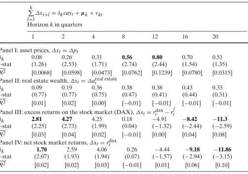
Table 5 Univariate long-horizon regressions on cay: components of asset wealth k l=1 ∆xt+l=δkcayt+µk+vkt Horizon k in quarters 1 2 4 8 12 16 20
Panel I: asset prices,∆xt=∆pt
δk 0.08 0.26 0.31 0.56 0.80 0.70 0.51
t-stat (1.26) (2.53) (1.71) (2.74) (2.44) (1.54) (1.35)
R2 [0.0068] [0.0598] [0.0473] [0.0762] [0.1239] [0.0780] [0.0315] Panel II: real estate wealth,∆xt=∆areal estatet
δk 0.09 0.19 0.36 0.38 0.38 0.43 0.33
t-stat (0.77) (0.77) (0.75) (0.47) (0.41) (0.44) (0.31)
R2 [0.01] [0.02] [0.00] [−0.01] [−0.01] [−0.01] [−0.01] Panel III: excess returns on the stock market (DAX),∆xt=rdaxt −rft
δk 2.81 4.27 4.25 0.18 −4.91 −8.42 −11.3
t-stat (2.25) (2.73) (1.99) (0.04) (−1.32) (−2.44) (−2.59)
R2 [0.03] [0.04] [0.02] [−0.01] [0.00] [0.04] [0.08] Panel IV: net stock market returns,∆xt=rdaxt
δk 1.70 2.59 4.06 0.26 −4.44 −9.18 −11.86
t-stat (2.07) (1.93) (1.94) (0.07) (−1.57) (−2.94) (−3.15)
R2 [0.02] [0.02] [0.03] [−0.01] [0.01] [0.06] [0.10] OLS regressions. t statistics are based on heteroskedasticity and autocorrelation consistent standard errors based on Newey and West (1987), using a window width of k+1. Panel I Our asset price measure is constructed as asset wealth net of cumulated savings: pt=at−tl=1ln(1+Yl−Cl/Al)
Panel III The risk free rate, rf, is a 3-months money market rate and rdax = ∆ln(DAXt)the quarterly returns on the DAX
the associated measure of fit compares very poorly with the results byLettau and Ludvigson(2001a,b), who report R2values for the net stock market return equation of up to 0.52 at business cycle frequencies and where the associated coefficients are robustly significant at all horizons.
It is important to emphasize that we are not saying that there is no transitory component in German asset prices. We just cannot identify these components based on the German cay. This point is borne out strongly by the results in Table6: here we also include the U.S. consumption–wealth ratio as constructed byLettau and Ludvigson(2001a,b) into the long-horizon regression for excess returns: both the German and the U.S. cay are strongly significant at horizons between 3 and 5 years and R2rises from 0.03 to reach 0.27 at a horizon of 12 quarters. The U.S. cay has considerable predictive power for excess returns in the German stock market. This suggests that there is considerable business-cycle variation in the German equity premium, but this variation displays an important international component.15
15 This ties in with recent results byNitschka(2004), who documents that the U.S. cay has consi-derable predictive power for the stock markets of the other G7 economies, including Germany.
Table 6 LH regressions of DAX excess returns on U.S. cay k
l=1
∆xt+l=δ1kcayGERt +δ2kcayUSt +µk+vkt
Horizon k in quarters
1 2 4 8 12 16 20
Panel I: excess returns on the stock market (DAX) -∆xt=rtdax−rft
δ1k 1.56 2.35 3.32 −1.29 −7.66 −11.48 15.74
t-stat (1.98) (1.81) (1.65) (−0.35) (−2.84) (−3.71) (−3.88)
δ2k 1.13 1.92 4.27 8.33 14.64 15.54 18.15
t-stat (1.43) (1.38) (1.46) (1.74) (2.83) (2.12) (1.85)
R2 [ 0.03] [0.04] [0.08] [0.10 ] [0.27] [0.25 ] [0.26 ] See Table5for notes
Our results so far suggest that cay is mainly related to cyclical fluctuations in income. We explore the implications of this point in our concluding section. Before, we briefly report on a battery of exercises that we undertook to check the stability and robustness of our results.
3.5 Stability and robustness issues
Data quality and interpolation: To rule out that data issues, in particular the
interpolation of our wealth data in the first half of the sample period affect our results, we did the following exercises: (i) run our analysis with only the CDAX variable (rather than the total wealth variable). (ii) run the system in four variables (stock market and non-stock market wealth separately) and, (iii) on annual (i.e. non interpolated) data. (iv) re-run our long-horizon regression for the subsample Q1:1992 to Q1:2004, using the re-estimated cay residual for this time span. Though rather short, this period offers us the advantage that non-interpolated quarterly data are available. (v) run the system with different consumption variables (i.e. excluding transportations and telecommunication). (vi) run the system with labour income instead of disposable income. None of the above mentioned exercises substantially affects our main result: income is the key variable driving the mean reversion on cay.
German unification: We also performed an extensive series of tests to check
to what extent German unification affects our results. Recursive estimation of the largest eigenvalue and the adjustment loadings clearly signal that there is one and only one cointegrating relationship throughout and that income is the single variable driving the error correction in the system. We also find the estimated cointegrating vector to be quite stable across subperiods, i.e. before and after German unification and with respect to the inclusion or exclusion of the late 90s technology bubble from the sample.
Q1-80 Q1-82 Q1-84 Q1-86 Q1-88 Q1-90 Q1-92 Q1-94 Q1-96 Q1-98 Q1-00 Q1-02 Q1-04 -0.05 -0.04 -0.03 -0.02 -0.01 0 0.01 0.02 0.03 0.04 cy cay
Fig. 2 Consumption–wealth ratio (cay) and detrended consumption income ratio (cy) for Germany
4 Discussion
4.1 Business cycles rather than stock market cycles
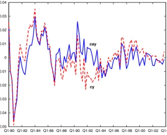
Our result that the German cay is mainly related to business cycles, not stock market cycles or the prices of other assets is somewhat reminiscent of
Cochrane’s(1994) finding that the consumption–income (GNP) ratio predicts cyclical fluctuations in U.S. GNP. In Fig.2we plot the cay residual against the consumption–income ratio, denoted with cy.16The correlation between the two time series is 0.8. This would seem to suggest that, in German data, the cay and
cy residuals contain the same information. To the extent that their fluctuations
signal changes in disposable income, and therefore in real economic activity, one might therefore expect that—in analogy to the findings inCochrane(1994)—
cay and cy should have predictive power for measures of the business cycle at
large.
In Table7we demonstrate that this is indeed the case. The table provides results from predictive regressions of a set of business cycle indicators on cy and the difference between the consumption–wealth and the consumption–income ratio, cay−cy. As is apparent from all four sets of regressions, the coefficient
on cay−cy is hardly ever significant, suggesting that it is mainly the variation
in cy that drives our findings.
While panel I just corroborates our earlier finding that income has an important transitory component, the results in panels II to IV show that c(a)y
has considerable forecasting power for other business cycle variables as well:
16 Under our maintained hypothesis, cay is stationary, whereas cy will not be. In what follows, we therefore detrend cy with a linear trend filter. Alternative detrending procedures, e.g. with the HP filter yield almost identical results.
Table 7 Regressions of business cycle indicators on cy and cay−cy k l=1 ∆xt+l=δ1kcyt+δ2kcayt−cyt+µk+vkt Horizon k in quarters 1 2 4 8 12 16 20 Panel I: income,∆xt=∆yt δ1k 0.31 0.58 0.88 1.41 1.67 1.47 1.26 (4.63) (5.21) (4.01) (5.10) (4.81) (4.12) (3.91) δ2k 0.15 0.26 0.28 0.17 −0.16 −1.26 −2.43 (1.09) (1.23) (0.80) (0.32) (−0.27) (−2.52) (−4.81) R2 [0.13] [0.24] [0.32] [0.42] [0.45] [0.49] [0.60] Panel II: GDP growth,∆xt=∆gdpt
δ1k 0.11 0.34 0.56 0.98 1.14 1.04 0.93 (1.44) (2.94) (2.36) (2.64) (2.06) (1.85) (1.38) δ2k 0.06 0.21 0.30 0.22 −0.04 −1.21 −2.34 (0.42) (0.83) (0.68) (0.36) (−0.04) (−1.33) (−1.91)
R2 [−0.01] [0.06] [0.09] [0.15] [0.15] [0.22] [0.30] Panel III: unemployment rate,∆xt=∆Ut
δ1k −0.08 −0.15 −0.31 −0.44 −0.44 −0.43 −0.47 (−3.61) (−3.34) (−3.73) (−2.23) (−1.95) (−2.13) (−2.31) δ2k −0.03 −0.05 −0.08 0.01 0.25 0.68 1.08
(−0.41) (−0.38) (−0.30) (0.03) (0.47) (1.32) (1.91)
R2 [0.08] [0.11] [0.16] [0.14] [0.14] [0.25] [0.41] Panel IV: private consumption deflator,∆xt=∆pcet
δ1k −0.14 −0.34 −0.49 −0.86 −1.04 −0.98 −0.73 (−2.07) (−2.85) (−2.10) (−2.83) (−2.75) (−2.31) (−1.95) δ2k −0.00 −0.03 0.13 0.35 0.87 1.53 2.20
(−0.03) (−0.14) (0.35) (0.51) (1.05) (1.85) (3.07)
R2 [0.10] [0.23] [0.21] [0.27] [0.35] [0.38] [0.40]
cy is the residual of a regression of ct−yton a constant and a linear trend. Further notes see Table5
while fluctuations in GDP (panel II) are not quite as predictable as income, we still attain an adjusted R2 of 15–30% at business cycle frequencies. The consumption–income ratio is also a successful predictor of the unemployment rate (panel III); again it is mainly cy that has predictive power and the regression accounts for 15–40% of the variability in unemployment at horizons between 2 and 4 years. Finally, cy also successfully predicts inflation in the deflator of private consumption expenditure with a measure of fit of 0.23 at horizons as low as two quarters.
4.2 The role of financial systems
Why is the German cay residual an indicator of business cycles rather than asset market fluctuations? One key explanation may be differences in financial systems:17Germany’s financial system is often characterized as bank-dominated
17 We refer the reader to the working paper version of this paper [Hamburg et al.(2005)] for a comprehensive discussion of these differences along with documenting statistical evidence.
while in Anglo-Saxon countries, such as the US, capital markets play a much bigger role for firms’ financing decisions [see e.g.Allen and Gale(2000)]. As a result, the German markets for both equity and corporate bonds are relatively small and the role of these two asset types in the net wealth position of the German private sector is minor. In addition, Germany’s public as well as most employer-sponsored retirement schemes are financed on a “pay as you go” basis. This further reduces the role of public equity holdings for retirement savings relative to the U.S. and other Anglo-Saxon countries, where private mutual funds and pension funds are much more prevalent.
4.3 The wealth effect on consumption
One point of departure for this paper was to quantify the magnitude of a poten-tial wealth effect on consumption in German data. Our analysis has highlighted that consumption does not seem to react to transitory shocks at all. To the extent that shocks to wealth are permanent, however, the effect on consumption can be gauged from the parameters of the cay relationship and from knowledge of the value of the ratio between consumption and asset wealth. To see this, note that the marginal propensity to consume out of wealth,ωt, is defined as
Ct =ωtWt=ωt(At+Ht)=ωtAt+ωtµtYt
whereωtµt defines the marginal propensity to consume out of income. From the above it is clear that the marginal propensity to consume out of total wealth just equals the marginal propensity to consume out of asset wealth, so that
ωt =∂Ct/∂At. From the cay relationship we know that the long-run elasticity of consumption with respect to asset wealth is just equal to the share of asset wealth in total wealth, the capital shareγ, so that
∂Ct ∂At At Ct =γ implying that ωt=γ Ct At
The annualized mean of Ct/At over our sample period is 0.1478, implying that the mean ofωtis 0.044: a one Euro increase in asset wealth leads to a 4–5 Euro cent increase in consumption spending per year. This number is in line with Ludvigson and Steindel(1999) who report a mean ofωt for the U.S. of 4–5%.
In our data set, asset wealth is predominantly permanent, whereas temporary fluctuations in income are the main driver of cyclical fluctuations in total wealth. Therefore, our estimate of 0.044 p.a. may capture the marginal propensity to consume out of asset wealth quite well, but is likely to be highly misleading with
respect to the marginal propensity to consume out of total wealth, or, for that matter, out of income.
A fully dynamic analysis of the interactions between consumption, asset wealth and income may be a more reliable guide to the wealth effect. In Fig.3
we plot impulse responses of c, a and y. These impulse responses are based on the decomposition of permanent and transitory shocks outlined in subsec-tion3.3. The transitory shock is readily identified fromτt=α −1εt. Since the adjustment coefficients on consumption (α1) and wealth (α2) are insignificant
according to our estimates in Table3, we restrictα =0, 0,α3
. A possible choice forα⊥is therefore given by
α⊥=
1 0 0 0 1 0
so that the vector of permanent shocks isπt = α⊥εt = [εct,εat]. This allows us to interpret the two permanent shocks as a shock to consumption (or total wealth) and a shock to asset wealth.18 Figure 3 provides a synopsis of the impulse responses, which for easier comparison are grouped by type of shock.
The response to the transitory shock is very much in line with our earlier findings: consumption and also asset wealth almost do not react, whereas the response of income is very marked and persistent.
After a permanent consumption shock, consumption reaches its new level immediately, whereas both asset wealth, but in particular income, reach their new permanent levels only gradually, after about 4–6 quarters. In accordance with economic theory, consumption ‘overshoots’ both asset wealth and income in the short run to adjust to its new permanent level immediately.
The second permanent shock is the shock to asset wealth. We interpret this shock as a temporary shock to asset returns. To underpin this interpre-tation, the respective panel in Fig. 3 also plots the impulse response of ∆p,
our comprehensive measure of asset price changes constructed in the pre-vious section. The response of∆p is hump-shaped but transitory. The shock
affects asset wealth and income asymmetrically, driving up asset wealth and driving down income. At the same time, it leaves consumption almost unaffec-ted. Note that the temporary return shock will still have a one-off permanent
18 The permanent shocksπ
tconstructed in this way are not necessarily mutually orthogonal. Their covariance isα⊥ α⊥= 11, where 11is the 2×2-matrix in the upper left corner of . For comparison and for the sake of interpretability, we also orthogonalize the permanent shocks
πt by obtaining the Choleski-factorization SCSC = 11. We further check for robustness by obtaining all possible orthogonalizations ofπtby rotating SC with an orthogonal matrix Q such that 11=SCQQSC. The matrix family Q can be represented as Q=
cosφ−sinφ sinφ cosφ
so that by lettingφvary on a grid, we can obtain all orthogonalizations of the permanent shocks. Whereas the impulse responses and variance decompositions we report in this subsection are based on Q=I, i.e. on the Choleski-factorization, the responses for the unorthogonalized shocks as well as the mean response over all realizations of Q turn out to be very similar.
0 5 10 15 20 -0.2 0.0 0.2 0.4 0.6 0.8 1.0 0 5 10 15 20 -0.2 0.0 0.2 0.4 0.6 0.8 1.0 0 5 10 15 20 -0.2 0.0 0.2 0.4 0.6 0.8 1.0
Consumption shock Wealth Shock
Transitory shock income consumption asset wealth asset wealth consumption income asset wealth consumption income returns
Fig. 3 Impulse responses of the VECM, synopsis by type of shock
effect on asset prices and therefore on asset wealth. It also drives down income permanently.19
To what extent are c, a and y driven by the permanent shocks? Figure 4
provides impulse responses again, this time including 90% confidence inter-vals obtained from 250 bootstrap replications of the VECM. The bootstrap results lend further support to our interpretation: the consumption shock is the only of the two permanent shocks to affect income and consumption signifi-cantly, whereas the return shock is the only permanent shock with a significant impact on asset wealth. Again, the transitory shock has a significant short-run effect only on income. In addition, variance decompositions based on an orthogonalized version of the identification outlined above (results not repor-ted) suggest that the asset wealth shock almost does not contribute to the
19 It may appear surprising that the return shock also leads to a permanent decline in income. Though, in view of the bootstrap results to be reported below, this result may not necessarily be significant, there could also be an interesting economic interpretation for it: if human (and in our case: proprietary) capital is non-tradeable, then—as argued inFisher and Voss(2004)—the discount factor to be applied to future income is just ra, the return on financial wealth. In this case, the cay-relationship simplifies to the following representation:
cay=Et ∞ j=1 ρjγra t+j+(1−γ )∆yt+j−∆ct+j
As cay is stationary, it is ultimately not affected by a permanent shock on assets, which is equivalent to a temporary return shock. Therefore, a positive temporary return shock must be offset by a tem-porary decrease in either consumption or income growth. Recall that consumption is unpredictable and does not react to the shock. Consequently, this alternative representation for cay implies that it must be income growth that falls temporarily, implying that the expected future level of income is reduced permanently.
0 10 20 -0.5 0 0.5 1 1.5 0 10 20 0 10 20 0 10 20 -0.5 0 0.5 1 1.5 0 10 20 0 10 20 0 10 20 -0.5 0 0.5 1 1.5 -0.5 0 0.5 1 1.5 -0.5 0 0.5 1 1.5 -0 .5 0 0.5 1 1.5 -0.5 0 0.5 1 1.5 -0 .5 0 0.5 1 1.5 -0.5 0 0.5 1 1.5 0 10 20 0 10 20 Consumption
cons shock return shock transitory shock
Assets
Income
Fig. 4 Impulse responses with bootstrapped confidence intervals
variation in consumption and income, whereas the consumption shock explains virtually all consumption variability at all horizons. It also explains most income variability in the long-run. The consumption shock can therefore also be inter-preted as a permanent income shock. This indicates that there is only a very limited direct effect of asset wealth on consumption in German data—a result that should caution against an over-interpretation of any estimate of the wealth effect that is based on a simple marginal propensity to consume.
5 Summary and conclusion
This paper has studied the link between consumption and wealth in Germany during the period 1980–2003. Very much as earlier studies for other countries, we can identify an empirical approximation of the consumption–wealth ratio as a cointegrating relationship between consumption, asset wealth and income—the
cay residual. In keeping with most versions of the permanent income
hypothe-sis, we find that consumption mainly reacts to permanent innovations in asset wealth and income. But whereas earlier studies for the U.S., Australia and the UK have documented that this cointegrating relationship predicts changes in asset prices, in particular risk premia in the stock market, we find that cay mainly predicts income changes in German data. Our explanation for this
phenome-non is that—probably due to structural differences in the financial and pension systems—stock market wealth accounts for a much smaller share of household net worth in Germany than in the Anglo Saxon economies so that temporary fluctuations in stock markets have only very limited impact on German private household net worth.
Since we find the consumption–wealth ratio to predict income rather than stock market fluctuations, one may expect cay to have forecasting power for many macroeconomic variables over the business cycle. Using a range of macroeconomic indicators for Germany, we have documented that this is indeed the case. Conversely, we find that temporary components in the German stock market can be identified with cyclical variation in the U.S. consumption– wealth ratio: variation in the German equity premium over the business cycle seems largely driven by international forces.
Our framework also allowed us to obtain an empirical measure of the wealth effect on consumption. Our estimates are in line with those reported for other countries: a one Euro increase in asset wealth leads to an increase in consump-tion spending by around 4–5 Euro cent. Such estimates can however be mis-leading if wealth has considerable transitory components. As our results have demonstrated, consumption reacts predominantly to permanent shocks. While German household asset wealth is indeed largely permanent, transitory shocks account for the bulk of variation in income at business cycle frequencies. Fur-thermore, permanent shocks to income rather than wealth seem to be the predominant driving force behind German private consumption.
Data appendix
Consumption and income Quarterly consumption and income data is avai-lable from the German national accounts.
Seasonally and working-day adjusted real disposable income of private households was obtained by taking the sum of seasonally and working-day ad-justed consumption and seasonally adad-justed savings, thus assuming that savings do not contain a calendar effect. As for the time before 1991 only annual dis-posable income is available, quarterly data was obtained using a cubic spline. All pre-1991 data is for West Germany only.
Besides net wages and salaries and net monetary transfers received dis-posable household income consists of net transfers from abroad and net other household income. Besides proprietary income, ‘net other income’ also includes other forms of capital income such as corporate dividend and interest payments. It would be desirable to disentangle these income components further. For the relatively long time period we require for our analysis, ‘other household income’ is, however, only available as an aggregate.
We also note that income data before 1980 are partly based on different SNA-definitions, and therefore the results reported in this paper are based on a sample ranging from 1980Q1 to 2003Q4.
Financial wealth Annual data for net financial wealth of the private sector according to ESA95 is available from the financial accounts [Bundesbank
(2004)] from 1991 onwards. Internally available quarterly data for net finan-cial wealth from 1991 onwards was used for the construction of our asset wealth variable. For the period before 1991 only annual West German data according to ESA79 can be obtained. The stock of shares and fixed-interest securities contained in this net financial wealth are at cumulated issue prices and nomi-nal values respectively. Thus, changes of wealth due to the variation of market prices are not adequately captured. However, stocks of shares and fixed-interest securities held by the private sector are available separately at current market prices. In order to picture the quarterly profile of net financial wealth at market values as adequately as possible, shares and fixed-interest security holdings at cumulated issue prices and nominal values were subtracted from net financial wealth. Quarterly data for the remaining variable, which is characterized by relatively little variation, was obtained by using a cubic spline. The series for shares at current market prices was then used to obtain quarterly values by assuming that its quarterly profile corresponds to the development of the stock market performance index CDAX. For fixed-interest securities the bond market index REX was applied to generate a quarterly profile. Both series were then added to the rest of net financial wealth in order to obtain quarterly data of net financial wealth of the private sector at market values for the time prior to 1991.
Housing wealth Residential housing wealth was obtained by combining capi-tal stock data from the German statistical office and a new price series that the Bundesbank calculates on the basis of information obtained from the Bulwien AG, which collects data on house prices in 60 German cities. These are weighted with population shares in order to construct house price indices.20 The index used here is for the typical object of newly built apartments and terraced houses of good quality. For the time before 1995 the index was calculated on the basis of information for West Germany only. As the price data is annual, a quarterly profile was also obtained by applying a cubic spline. Capital stock data was constructed from annual data on gross fixed assets of residential housing (dwel-lings) at 1995 prices that is only available for all sectors combined and thus slightly overestimates the assets held by the private households. The quarterly profile was obtained by using the corresponding seasonally adjusted residen-tial investment series from the national accounts. The implied annual capital consumption was calculated and assumed to follow a smooth quarterly path. Combining this with the quarterly investment data from the national accounts, a quarterly capital stock series could be generated. The series was extended backwards into the period before 1991 using growth rates obtained from West German data on fixed assets of residential housing at 1991 prices that is only available according to a slightly different statistical concept from the “dwel-lings” of the German data. Again, a quarterly profile of this data was obtained by applying a cubic spline.
References
Allen FD, Gale D (2000) Comparing financial systems. MIT, Cambridge
Becker S, Hoffmann M (2006) Intra- and international risk-sharing in the short run and the long run. Eur Econ Rev 50:777–806
Beveridge S, Nelson CR (1981) A new approach to decomposition of economic time series into permanent and transitory components with particular attention to measurement of the business cycle. J Monet Econ 7:151–174
Campbell JY, Cochrane JH (1999) By force of habit: a consumption-based explanation of aggregate stock market behavior. J Polit Econ 107:205–251
Campbell JY, Mankiw GN (1989) Consumption, income, and interest rates: reinterpreting the time series evidence. In: Blanchard O, Fischer S (eds) NBER macroeconomics. MIT, Cambridge, pp 185–216
Cochrane JH (1994) Permanent and transitory components of GDP and stock prices. Q J Econ 109:241–265
Cochrane JH (2001) Asset pricing. Princeton University Press, Princeton
Constantinides G, Duffie D (1996) Asset pricing with heterogeneous consumers. J Polit Econ 104:219–240
Bundesbank D (2003a) New price indices for housing in Germany. Mon Rep 5:38 Bundesbank D (2003b) Price indicators for the housing market. Mon Rep 9:45–58
Bundesbank D (2004) Ergebnisse der gesamtwirtschaftlichen Finanzierungsrechnung für Deut-schland 1991 bis 2003
Fernandez-Corugedo E, Simon P, Blake A (2003) The dynamics of consumers’ expenditure: the UK consumption-ECM redux. Bank of England Working Paper 204
Fisher LA, Voss GM (2004) Consumption, wealth and expected stock returns in Australia. Econ Rec 80:359–372
Gonzalo J, Granger CW (1995) Estimation of common long-memory components in cointegrated systems. J Bus Econ Stat 13:27–35
Guo H (2001) A simple model of limited stock market participation. Federal Reserve Bank of St. Louis Review May/June 37–47
Hamburg B, Hoffmann M, Keller J (2005) Consumption, wealth and business cycles: why is Germany different? Deutsche Bundesbank Discussion paper 16/2005
Heaton J, Lucas D (2000) Portfolio choice in the presence of background risk. Econ J 110:1–26 Hoffmann M (2001) Long run recursive VAR models and QR decompositions. Econ Lett 73:
15–20
Hoffmann M (2006) Proprietary income, entrepreneurial risk and the predictability of stock returns. Cesifo Working Paper:1712
Johansen S (1995) Likelihood-based inference in cointegrated vector autoregressive models. Oxford University Press, Oxford
Johansen S, Nielsen B (1993) DisCo. Institute of Mathematical Statistics, University of Copenhagen Lettau M, Ludvigson S (2001) Consumption, aggregate wealth and expected stock returns. J Financ
56:815–849
Lettau M, Ludvigson S (2001) Understanding rrend and cycle in asset values: Reevaluating the Wealth Effect on Consumption. Am Econ Rev 94:276–299
Ludvigson S, Steindel C (1999) How important is the stock market effect on consumtpion? FRBNY Econ Policy Rev 7:29–51
Lütkepohl H(2005) New introduction to multiple time series analysis. Springer, Berlin
Modigliani F (1971) Consumer spending and monetary policy: the linkages. Federal Reserve Bank of Boston Conference Series
Newey WK, West KD (1987) A simple, positive semi-definite, heteroskedasticity and autocorrela-tion consistent covariance matrix. Econometrica 55:703–708
Nitschka T (2004) The U.S. consumption wealth ratio and the predictability of international stock markets: evidence from the G7. mimeo, University of Dortmund
Polkovnichenko V (2004) Limited stock market participation and the equity premium. Financ Res Lett 1:24–34