Adaptive Varying-Coefficient Linear Models

ADAPTIVE VARYING-COEFFICIENT LINEAR MODELS

by

Jianqing Fan

1

Department of Statistics, University of North Carolina, Chapel Hill

Qiwei Yao

2

Department of Statistics, London School of Economics and Political Science

Zongwu Cai

Department of Mathematics, University of North Carolina, Charlotte

Contents:

Abstract

1. Introduction

2. Overview of varying-coefficient modesl

3. Adaptive varying-coefficient linear models

4. Varying-coefficient linear models with

two indices

5. Numerical properties

Appendix: Proof of Theorem 1

References

Figure 7(a)

The Suntory Centre

Suntory and Toyota International Centres

for Economics and Related Disciplines

London School of Economics and Political Science

Discussion Paper

Houghton Street

No. EM/00/388

London WC2A 2AE

April 2000

Tel.: 020 7405 7686

1

Supported partially by NSF grant DMS-9803200.

2

Supported partially by EPSRC Grant L16385 and BBSRC/EPSRC Grant

96/MMI09785.

We thank Professors N C Stenseth and A R Gallant for making available Canadian

mink-muskrat data and pound/dollar exchange data analysed in Section 4.2.

Abstract

Varying-coefficient linear models arise from multivariate nonparametric

regression, nonlinear time series modelling and forecasting, functional data

analysis, longitudinal data analysis, and others. It has been a common

practice to assume that the vary-coefficients are functions of a given variable

which is often called an index. A frequently asked question is which variable

should be used as the index. In this paper, we explore the class of the

varying-coefficient linear models in which the index is unknown and is

estimated as a linear combination of regression and/or other variables. This

will enlarge the modelling capacity substantially. We search for the index such

that the derived varying-coefficient model provides the best approximation to

the underlying unknown multi-dimensional regression function in the least

square sense. The search is implemented through the newly proposed hybrid

backfitting algorithm. The core of the algorithm is the alternative iteration

between estimating the index through a one-step scheme and estimating

coefficient functions through a one-dimensional local linear smoothing. The

generalised cross-validation method for choosing bandwidth is efficiently

incorporated into the algorithm. The locally significant variables are selected

in terms of the combined use of t-statistic and Akaike information criterion. We

further extend the algorithm for the models with two indices. Simulation shows

that the proposed methodology has appreciable flexibility to model complex

multivariate nonlinear structure and is practically feasible with average

modern computers. The methods are further illustrated through the Canadian

mink-muskrat data in 1925-1994 and the pound/dollar exchange rates in

1974-1983.

Keywords: Akaike information criterion; backfitting algorithm; generalised

cross-validation; local linear regression; local significant variable selection;

one-step estimation; smoothing index; varying-coefficient linear models.

JEL No.: C22

©

by the authors. All rights reserved. Short sections of text, not to exceed two

paragraphs, may be quoted without explicit permission provided that full

credit, including © notice, is given to the source.

During the recent years, with increasing computing power it has become commonplace to access

and to attempt to analyze data of unprecedented size and complexity. With these changes has

comean increasingdemandforthedevelopment ofcomputationallyintensivemethodologieswhich

are designed to identifycomplicated data structures at not too excessive computing cost.

Data-analytic techniques developed from statistical prospective views have been proved powerful for

exploiting hidden structures in high-dimensional data. Witness of this includes, among others,

additive modeling (Breiman and Friedman, 1985; Hastie and Tibshirani, 1990), low-dimensional

interaction modeling (Friedman, 1991; Gu and Wahba, 1993; Stone et al., 1996), multiple-index

models (Friedman and Stuetzle, 1991; Hardle and Stoker, 1989; Li, 1991), partiallylinear models

(Wahba,1984;GreenandSilverman,1994),varying-coeÆcientlinearmodels(Clevelandetal.,1992;

Hastie and Tibshirani, 1993), and their hybrids(Carroll et al., 1997; Fan Hardle and Mammen,

1998). Those modelsare designed to attenuate the so-called`curse of dimensionality' problemby

exploring low-dimensional structures, although dierent modelsexplore dierent aspects of

high-dimensionaldata and incorporate dierent priorknowledge. The aim of theexercises isto reduce

possiblemodelingbias and to let dataselect a model whichdescribesthemselves well. Depending

on each particular data set, some methodsperform better and are more appropriate to use than

others, but none of them is uniformly superior. They together provide useful statistical toolkits

forexploringhiddenstructuresinhigh-dimensionaldata. Forgeneral knowledge ofnonparametric

and semi-parametricmodelingtechniques, we refer to thebooks by Hastieand Tibshirani(1990),

Wahba (1990), Greenand Silverman(1994), Wand and Jones (1995), Fan and Gijbels(1996) and

Simono (1996).

Supposewe are interested inestimating multivariateregression functionG(x ) E(YjX=x),

where Y is a random variable and X is a d1 random vector. In this paper, we propose to

approximatetheregression functionG(x) bya varying-coeÆcientmodel

g(x)= d X j=0 g j ( T x)x j ; (1.1) where2< d is anunknowndirection,x=(x 1 ;:::;x d ) T ,x 0 =1,and coeÆcients g 0 ();:::;g d ()

are unknown functions. We choose the direction and coeÆcient functions fg j

()g such that

EfG(X) g(X )g 2

obtains its minimum. The appeal of this model is that once is known, we

can directly estimate g j

() 0

s by the standard one-dimensional kernel regression localized around

T

x. Furthermore,thecoeÆcientfunctions fg j

()g can beeasilydisplayedgraphically,whichmay

be particularly helpful to visualize how the surface g() changes. The model (1.1) appears linear

in each coordinates of x when the index T

x is xed. It may include additional quadratic and

cross-product terms of x 0 j

s (or more generally any given functions of x 0 j

s)as `new' components of

x. Henceit isinfact considerablyexibleto cater to complexmultivariatenonlinearstructure.

1975) and estimating functions fg j

()g through a one-dimensional local linear smoothing. Since

we apply smoothing on a scalar T

X only, the method suers little from the so-called `curse of

dimensionality'which is the innate diÆculty associated with multivariatenonparametric ttings.

The generalized cross-validation method (GCV) for bandwidth selection is incorporated into the

algorithm in an eÆcient manner. To avoid over-tting, we delete local insignicant variables in

termsofthecombineduseoft-statisticandAkaikeinformationcriterion(AIC).Thisisparticularly

important when we include, for example, quadratic functions of x 0 j

s as new components in the

model,whichcouldlead to overparametrization. Theproposedmethodhasbeenfurtherextended

to estimate varying-coeÆcient modelswithtwoindices(oneof them isknown).

The form of the model (1.1) is not new. It was proposed in Ichimura (1993). Recently, Xia

and Li (1999a) extended the idea and the results of Hardle, Hall and Ichimura (1993) from the

single-indexmodel to the adaptive varying-coeÆcient model (1.1). Their basicidea is to estimate

thecoeÆcientfunctionswithagivenbandwidthandadirection,andthenchoosethebandwidth

and thedirection by the cross-validation. Based on the assumption that thebandwidth is of the

order O(n 1=5

) and the direction is within an O p

(n 1=2

) consistent neighborhood of the true

value, they obtained some interesting theoretical results. However, the approach suers from the

heavy computational expenses. This somehow explains why most previous work focused on the

case when the direction is given and is parallel to one of coordinates. See x2 for an overview.

The new approach inthis paperdiersfrom those inthe literaturein three key aspects: (a) only

one-dimensional smoother is used in estimation, (b) the index coeÆcient is estimated by data

and (c) within a local region around T

x, we select signicant variables x 0 j

s to avoid overtting.

Aspect (b) is dierent from Hardle, Hall and Ichimura (1993) and Xia and Li (1999a) since we

estimate the coeÆcient functions and the direction simultaneously; no cross-validation is needed.

This idea is similar in spirit to that of Caroll et al. (1997) who showed that a semiparametric

eÆcient estimator of the direction can be obtained via this approach. Further we provide a

theorem (i.e. Theorem 1(ii) in x3 below) on the model identication problem of the form (1.1),

which hasnotbeenaddressed before.

The applicationofvarying-coeÆcientmodelsisdiverse;rangingovergeneralized linearmodels,

nonlinear time series, functional data analysis, longitudinal data analysis, and other

interdisci-plinaryareas. Whiletheseproblemsareinnerrelated,they arenotoftenreferredto eachother. In

x2,wewillgiveanoverviewonthecurrentstate-of-artofthevarying-coeÆcientmodelsinpractice.

The rest of the paper is organized as follows. x3 deals with the adaptive varying-coeÆcient

model (1.1). Theextension to theadaptive varying-coeÆcientmodelsto thecase withtwo indices

is outlined in x4. The numerical results of three simulated examples are reported in x5.1, which

demonstratethattheproposedmethodologyiscapabletocapturecomplexnonlinearstructurewith

moderate samplesizes,andfurthertherequiredcomputationtypicallytakeslessthanaminuteon

mink-proofsare relegated intheAppendix.

2 Overview of varying-coeÆcient models

Varying coeÆcient models have beensuccessfully applied to multi-dimensional nonparametric

re-gression, generalized linearmodels, nonlineartimeseriesmodels,longitudinaland functionaldata

analysis, interest rate modeling in nance, international conict study in political sciences and

others. The basic idea is to approximate a unknown multi-dimensional regression function by a

(conditionally) linearmodel withthecoeÆcientsbeingfunctions ofa covariatecalledindex. Most

oftheworkto dateassumesthat theindexis given. Theadaptivevarying-coeÆcientmodelsallow

datatochoosetheindexautomatically. Thissectionpresentsanoverviewontherecentdevelopment

of thevarying-coeÆcientmodels.

2.1 Varying coeÆcient models

The varying-coeÆcient models were introduced by Cleveland, Grosse and Shyu (1992) in the

ex-tension oflocalregression techniquesfrom one-dimensionalto multi-dimensionalsetting. Suppose

that we are given a random sample f(U i ;X i ;Y i );1 i ng, where Y i

is the response variable

and (U i

;X i

) are covariates. The local polynomial regression essentially tsthe conditional linear

model Y i = d X j=0 g j (U i )X ij +" i ; (2.1) whereX ij isthej-thcomponentof X i ,X i0 1,and" i

hasconditional meanzeroand conditional

variance 2 (U i ), given U i and X i

. The coeÆcient functions fg j

()g are assumed to be smooth.

An extension of the local regression technique was given by Hastie and Tibshirani (1993) via

introducingkernel weights. Let K() be a kernel function on < and h =h n be a bandwidth. Set K h ()=h 1 K(=h). For agiven u 0 and xclose to u 0

,it followsa Taylorexpansionthat

g j (x)g j (u 0 )+g 0 j (u 0 )(x u 0 )b j +c j (x u 0 ): (2.2)

Here, the only local linear approximation is used for the sake of simplicity. It can be easily

gen-eralized to the local polynomialregression (Fan and Gijbels, 1996). Thus, forthose observations

whereU 0 i

s are aroundu 0

,thedatafollowan approximationlinear model:

Y i d X j=0 fb j +c j (U i u 0 )gX ij +" i :

The localparameters can beestimated via aweighted localregression,namely

b g j (u 0 )= b b j ; j=0;:::;d; (2.3)

wherefb j

;bc j

gis theleast-squaressolutionwhichminimizes

n X i=1 h Y i d X j=0 fb j +c j (U i u 0 )gX ij i 2 K h (U i u 0 ): (2.4)

The conditional bias and variance of the estimators were derived in Caroll, Ruppert and Welsh

(1998) and Fan and Zhang (2000a). As expected, the bias depends only on local approximation

errorandisoforderO(h 2 n

),andthevarianceisoforderO(1=(nh))anddependsonlyontheeective

number of local data points, the local (conditional) variance and local correlation matrix of the

covariates X. The asymptotic normality of the estimators and data-driven bandwidth selection

procedure were presented in Zhang and Lee (1999, 2000). Furthermore, the distribution of the

maximum discrepancy between the estimated coeÆcients and true coeÆcients was discussed by

Xia and Li (1999b) and Fan and Zhang (2000b). The condence bands and hypothesis testing

problemswerealso discussedtherein.

Complementaryto thelocal regression techniqueis thesmoothingsplinesmethod. Hastie and

Tibshirani(1993) proposedasmoothingsplineestimator derived via minimizing n X i=1 n Y i d X j=0 g j (U i )X ij o 2 + d X j=0 j kg 00 j k 2 2 ; (2.5) where f j

g are positive regularization parameters. As an initial attempt, one usually chooses

j

=for all j. Notethat thelocal regression solvesmany(usually intheorder of 100)weighted

regression problems(2.4),whilethesmoothingspline methodsolvesone largeparametric problem

(numberof parametersis intheorder ofnd).

The local regression estimator (2.3) assumes implicitly that the coeÆcient functions fg j

()g

admit a similar degree of smoothness so that they can be equally well approximated in a local

neighborhood (see (2.2)). When the functions fg j

()g have dierent degrees of smoothness, it is

showninFanand Zhang(2000a)thatthelocalregressionestimator(2.3) issuboptimalundertheir

asymptotic formulation. The intuition is clear: a smooth component asks for a large bandwidth

to reduce the variance, whilea rough component requires a small bandwidthto reduce the bias.

This problemcannot be overcome by, for example, simply usinga largebandwidth to estimating

a smooth component only; see Fan and Zhang (2000a). While the asymptotic properties for the

smoothingspline estimator (2.3) are not easy to derive, we expect that smoothing splines would

suer from thesame problemeven when f j

gare appropriately specied. However thedrawback

can beremoved byusinga two-stepprocedureproposedinFanand Zhang(2000a). Thebasicidea

isto getan initialestimatorforfbg j

()gusingasmallbandwidthh 0

. Thebandwidthh 0

issosmall

thatthe biasesinestimationof fbg j

()g are negligible. Then,computethe partialresiduals

b Y i;j =Y i X k6=j b g k (U i )X ik

and applythelocal linearregression technique to thepseudounivariatevarying-coeÆcient model

b Y i;j =g j (U i )X ij +" i

j j j nowbeselected purposelyforestimatingg

j

()onlyand univariatebandwidthselectiontechniques

can beapplied.

When themodel (2.1)is misspecied,theabove localttingtechniquesintendto ndthebest

linear function at each given U = u 0

to approximate the regression function E(YjU = u;X).

Similarly,thesmoothingspline(2.5) ndsthebestvarying-coeÆcientfunctionto approximatethe

regression surfaceE(YjU; X).

In nonparametric modeling, we are constantly challenged by the question whether a simpler

parametric model ts the data adequately or not. For example, we may ask if the coeÆcients in

themodel(2.1) areall constant. This amounts to testingthe parametrichypothesis

H 0 :g j ()= j ; j =0;:::;d;

against nonparametric alternative (2.1). We can also ask whether the covariates X 1

and X 2

are

signicant. This isequivalent to testing

H 0 :g 1 ()=0 and g 2 ()=0:

In thiscase, both nulland alternative hypotheses arenonparametric. While these questions arise

frequentlyinpractice,theyarepoorlyunderstood. Theconventionalapproachusesthediscrepancy

measuressuchasthedistancesbetweenestimatedfunctionsundernullandalternative hypotheses.

See,forexample,BickelandRosenblatt(1973), HardleandMammen(1993)andHart(1997). Fan,

Zhang and Zhang (1999) argued that these methods were not as fundamental as the likelihood

ratio based statistics. Generalized likelihood ratio tests are proposed there for various

nonpara-metric testing problems and the Wilks phenomenon and optimality properties are unveiled. The

basicideaofthegeneralizedlikelihoodratiotestsistondgoodestimatorsunderthenulland full

modelsand thensubstitute them into thelikelihoodfunctionto obtainalikelihoodratiostatistic.

Afundamentalpropertyofthederivedtest isthattheasymptoticnulldistribution isindependent

of nuisance functions and is 2

-distributed. This allows usto use either the asymptotic null

dis-tribution or bootstrap methods to determine the p-values of the tests. See also Cai, Fan and Li

(2000) forbootstrap estimationofnulldistributionsand empiricalpowercalculations.

2.2 Generalized varying-coeÆcient models

VaryingcoeÆcient modelscan be readilyextended tothecontext of thegeneralized linearmodels.

Thisallows usto model atransform oftheregression functionbya varying-coeÆcient model

`fE(YjU;X )g= d X j=0 g j (U)X j

withagiven linkfunction`(), whereX 0

=1. TheunknowncoeÆcient functionscan beestimated

viewed asa specic case of thelocal estimation equation method of Carroll, Ruppert and Welsh

(1998). The splinemethod can also be appliedinthiscontext (Hastie and Tibshirani,1993).

Carroll,RuppertandWelsh(1998)derivedtheasymptoticexpressionsforconditionalmeanand

varianceforthelocalequation estimators. Theresultscanbeextendedto thegeneralized

varying-coeÆcient modelswith some additional work. Cai, Fan and Li (2000) established theasymptotic

normalityof the local maximum likelihood estimator. They also proposed a fast implementation

algorithm based on a one-step local maximum likelihoodestimator. The basicidea is to compute

genuinelocalMLEsatafewwell-separategridpointsandthentousethemasinitialvaluesforthe

localMLEsattheirnearestgridpointsviaone-stepNewton-Raphsoniteration. Theestimatesatall

gridpointsareobtainedbyrepeatingtheaboveexerciseinwhichanewlydenedestimateistreated

as an initial estimate at its next grid point. Cai, Fan and Li (2000) showed that this estimator

shares the same asymptotic behavior as the genuine local likelihood estimator. Kauermann and

Tutz (1999) proposed a graphical technique to diagnose the discrepancy between a parametric

model and a varying-coeÆcient model. Cai (1999) used a two-step procedure to deal with the

situationwherethecoeÆcientfunctionsfg j

()gadmitdierentdegreesofsmoothness. Thetesting

procedure and estimation method in Cai, Fan and Li (2000) have been successfully applied by

Cedermanand Penubarti(1999) tothestudyof internationalrelationconictinpoliticalsciences.

2.3 Nonlinear time series

Varying-coeÆcientmodelshavebeenelegantlyappliedtomodelingandforecastingtimeseriesdata

(Nichollsand Quinn,1982;Chen and Tsay,1993). They arenaturalextensions of thethresholded

autoregression modelsofTong (1990). Let fX t

gbe atime series. The varying-coeÆcient modelis

of form X t =g 0 (X t p )+ d X j=1 g j (X t p )X t j +" t (2.6)

forsome givenlagsd andp. Thegeometricergodicityof thismodelwasstudiedbyChenandTsay

(1993), who also proposed a nearest neighborhood type of estimator. The local linear regression

estimation (2.4) applies readily to this autoregressive setting. The asymptotic normality of such

an estimator has been establishedin Cai, Fan and Yao (1998). They also proposed a generalized

pseudo-likelihoodtestfortestinglinearautoregressivemodelsorthresholdedmodelsagainstmodel

(2.6). The procedure is basically the same as the generalized likelihood ratio statistic for the

independent data, but now adapts to the time series setting. A bootstrap method is used to

estimatetheasymptoticnulldistribution. Thetestingprocedureandestimationmethodhavebeen

successfullyappliedbyHongand Lee(1999) totheinferenceandforecastof exchangeratesand by

Inmanyapplications,observationsfordierentindividualsarecollectedoveraperiodoftime. The

numberofobservationsfordierent individualsmaybe dierentand soisthetimewhen thedata

arerecorded. Thistype of dataistermed aslongitudinaldata. Often, interestliesinstudyingthe

association betweenthe covariates and theresponse variable. To this end,a linear modelis often

employed: Y i (t ij )= 0 +X i (t ij ) T +" i (t ij ); (2.7) where (X i (t ij );Y i (t ij

)) is the observed datum for the ith individual at time t ij and " i (t ij ) is the

stochastic noise. The key dierence from cross-sectional data is that the error process f" i

(t ij

)g

within subject i is correlated. See, for example, Diggle, Liang and Zeger (1994) and Hand and

Crowder(1996).

Despite of its success in many applications, the model (2.7) does not allow the association

to vary over time, even though the covariates and the response variable change over time and

environment. Toaccountforthis,ZegerandDiggle(1994)andMoyeedandDiggle(1994)proposeda

semiparametricmodelwhichallowstheintercept 0

tovaryovertime,butnottheothercoeÆcients.

To facilitate the genuine variation of the association over time, Brunback and Rice (1998) and

Hooveretal. (1998) proposedto usethevarying-coeÆcient model

Y i (t ij )= 0 (t ij )+X i (t ij ) T (t ij )+" i (t ij ); (2.8)

where the coeÆcient functions are assumed to be smooth functions of time. This is a specic

case of the functional linear model discussed in Ramsay and Silverman (1997) in the context of

functional data analysis. When there is no covariate, the model (2.8) was studied by Hart and

Wehrly (1986, 1993) for repeated measurements and byRice and Silverman (1991) for functional

data. There themean regression was estimated by the kernel and smoothingspline methods. A

`deleting one-subject each time' cross-validation was proposed in Rice and Silverman (1991) for

choosingsmoothingparameters.

ThecoeÆcientsinthemodel(2.8)canbeestimatedbythekernelandsmoothingsplinemethods

(BrumbackandRice,1998;Hooveretal.,1998). Thebasicideaisthesameasthoseoutlinedinx2.1.

BrumbackandRice (1998)pointedoutthatintensivecomputationisrequiredforusingsmoothing

splinesbecause one has to invertblindly a matrixof the order of thetotal number of datapoints

(i.e. sum of the number of repeated measurements for each individual). Fan and Zhang (2000)

proposed a two-stepmethod to overcome thisdrawback. Thebasicidea is relatedto thetwo-step

method outlinedin x2.1, butnowadapts to longitudinaldata setting. For eachdistinct datatime

pointt j

,collectthesubjectshavingobservationsattimet j

(ormoregenerallyaroundt j

)andtthe

linearmodel(2.7)forthosedatapoints. ThisgivesustheinitialestimatedcoeÆcientsattimet j

. In

thesecondstep, insteadofsmoothingon thepartialresiduals,theinitialestimated coeÆcientsare

asymptoticbiasand varianceofkernelmethodwasstudiedbyHooveret al. (1998). Furthermore,

Wu, Chiangand Hoover(1998) proposedapproaches forconstructing condenceregions based on

thekernelmethod.

3 Adaptive varying-coeÆcient linear models

3.1 Approximation and identiability

Since G(x)=E(Y jX=x)is aconditional expectation,itholdsthat

EfY g(X)g 2 =EfY G(X )g 2 +EfG(X) g(X )g 2

for any g() with nite second moment. Therefore, the search for the LS approximation g() of

G(), as dened in (1.1), is equivalent to the search for such a g() that EfY g(X)g 2

obtains

its minimum. Theorem1(i) below indicatesthat there always existssuch a g() under some mild

conditions. Obviously,ifG(x) isintheformoftheRHS of(1.1), g(x)G(x). Thesecond partof

thetheorempointsoutthatthecoeÆcientvectorisuniqueuptoaconstantunlessg()isinaclass

of special quadratic functions (see (3.2) below). In fact, the model (1.1) is an over-parametrized

form in the sense that one of fg j

()g can be represented in terms of the others. Theorem 1(ii)

conrms thatoncethedirection isspecied,thefunctiong() hasarepresentationwithat most

d (instead ofd+1) g j

()-functions. Furthermore,those g j

()-functionsareidentiable.

Theorem 1. (i) Assume that the distribution function of (X ;Y) is continuous, and EfY 2

+

jjXjj 2

g<1. Then,there existsa g() denedby(1.1) forwhich

EfY g(X)g 2 =inf inf f 0 ;:::;f d E 8 < : Y d X j=0 f j ( T X)X j 9 = ; 2 ; (3.1)

where the rst innitumis taken over all unit vectors in < d

, and the second over all measurable

functions f 0

();:::;f d

().

(ii) For any given twice dierentiable g() of the form (1.1), if we choose jjjj = 1, and the rst

non-zerocomponent of positive, sucha isunique unlessg() isof theform that

g(x)= T x T x+ T x+c; (3.2) where; 2< d

,c2<areconstants, and and arenotparallelwitheachother. Furthermore,

once = ( 1 ;:::; d ) T is given and d 6= 0, we may let g d

() 0. Consequently, all the other

g j

() 0

s areuniquelydetermined.

Remark 1. If theconditional expectation G(x) =E(YjX=x) cannot be expressedin the form

of the RHS of (1.1), there may exist more than one g(x) 0

s, being of the form of (1.1), for which

(3.1) holds. For example, let Y = X 2 1 +X 2 2 , where both X 1 and X 2

variables uniformly distributed on [0;1]. Then G(x 1 ;x 2 ) = x 1 +x 2

, which is not of the form of

varying-coeÆcientlinearmodel(1.1). However,(3.1)holdsforbothg(x 1 ;x 2 )=1:25x 2 1 ,and1.25x 2 2 .

Without lossofthegenerality,wealwaysassumefrom nowonthatinthemodel(1.1),jjjj=1

and therstnon-zerocomponent of ispositive. Toavoidthecomplicationcaused bythelackof

uniquenessoftheindexdirection,wealwaysassumethatG()admitsauniqueLSapproximation

of g() which cannotbeexpressed intheform of(3.2).

3.2 Estimation

Supposethatf(X t

;Y t

); 1tngareobservationsfromastrictlystationaryprocess,and(X t

;Y t

)

hasthesame marginaldistributionas(X;Y). Ofinterestisto estimatethesurfaceg()denedby

(1.1) and (3.1). It is clear from (3.1) that we needto search forthe minimizersof ff j

()g for any

givendirection andthenndthedirectionatwhichthemeansquarederror(MSE)isminimized.

Agenuinesearchisalmostalwaysintractableinpractice. Weadaptaback-ttingalgorithmwhich

has been demonstrated to be eÆcient for solving such a computationally intensive optimization

problem.

Weassumethat d

6=0. ItfollowsfromTheorem1(ii)thatweonlysearchforanapproximation

intheform g(x)= d 1 X j=0 g j ( T x)x j ; (3.3)

sincethetermg d

( T

x)x d

can beexpressedasalinearcombinationofterms in(3.3). Our taskcan

be formally split into two parts | estimation of functions g j

() 0

s with given and estimation of

theindex coeÆcient withgiven functions fg j

()g. We also discusshowto choose thesmoothing

parameter h, and how to apply backward deletion to choose locally signicant variables. The

algorithm forpracticalimplementationwillbe summarizedat theendof thissection.

3.2.1 Local linear estimators for g j () 0 s with given Forgiven with d 6=0,we needto estimate g(X)=arg min f2F() E h fY f(X)g 2 T X i ; (3.4) where F()= 8 < : f(x)= d 1 X j=0 f j ( T x)x j f 0 (); :::;f d 1

()measurable; and Eff(X)g 2 <1 9 = ; : (3.5)

The least-squares property in (3.4) suggests the estimators bg j (z) = b b j , j = 0; :::;d 1, where b b 0 ;:::; b b d 1

istheminimizer ofthe sumof weightedsquares

n X t=1 8 < : Y t d 1 X j=0 b j X tj 9 = ; 2 K h ( T X z)w( T X t );

boundaryeect. Since T

X isobservable when is given, theestimationof g j

() 0

s byminimizing

theabove sum of squarescan beviewed as an extension ofstandard kernel regression estimation.

Infact,byimposingaspeciedstructureontheformofg(),weareableto transfertheestimation

of amultivariatefunction into theestimationof several univariatefunctions. Therefore, only

one-dimensionalkernelsmoothingisinvolved.

The above estimation procedure is based on the local constant approximation: g j

(y) g j

(z)

foryinaneighborhoodofz. Ithasbeenpointedoutthatthelocalconstant regressionhasseveral

drawbacks comparing with local linear regression (Fan and Gijbels, 1996). Therefore we consider

thelocallinearestimators forfunctionsg 0

();:::;g d 1

(). Thisleadsto minimizingthesum

n X t=1 2 4 Y t d 1 X j=0 n b j +c j ( T X t z) o X tj 3 5 2 K h ( T X t z)w( T X t ) (3.6) withrespecttofb j gand fc j

g. Dene theestimators b g j (z)= b b j and b _ g j (z)= b c j forj=0;:::;d 1 and set b b b 0 ; :::; b b d 1 ; b c 0 ;:::; b c d 1 T :

It followsfrom theleast squarestheorythat

b =(z)X T (z)W(z)Y; and (z)=fX T (z)W(z)X(z)g 1 ; (3.7) where Y = (Y 1 ;:::;Y n ) T

, W(z) is an nn diagonal matrix with K h ( T X i z)w( T X i ) as its

i-th diagonal element, X(z) is an n2d matrix with (U T i ;( T X i z)U T i

) as its i-th row, and

U t =(1;X t1 ;:::;X t;d 1 ) T .

3.2.2 Search for -direction with g j

() 0

s xed

The minimizationpropertyin(3.1) suggests thatwe shouldsearch for forwhich thefunction

R ()= 1 n n X t=1 8 < : Y t d 1 X j=0 g j ( T X t )X tj 9 = ; 2 w( T X t ) (3.8)

obtainsitsminimum. Infact,we willusetheestimatorsoffg j

()g whichcannotbeestimatedwith

reasonable accuracy at the tails. Obviously, a genuine exhaustive search willbe a forbiddentask

even formoderate d. A simplewayoutis to employone-stepestimationscheme (see,forexample,

Bickel, 1975). The proposedmethod is in thespirit of one-step Newton-Raphsonestimation. We

anticipatethatthe derived estimator performswelliftheinitialvalue isreasonablygood (seeFan

and Chen,1997). We outline theprocedure below.

Supposethat b

is the minimizer of(3.8). Then _ R b =0, where _

R ()denotes thederivative

of R (). For any (0)

close to b

,we have theapproximation

0= _ R ( b ) _ R (0) +  R (0) b (0) ;

where R () is the Hessian matrix of R (). The above observation leads us to dene the one-step

iterative estimatefor as

(1) = (0) n  R (0) o 1 _ R (0) ; (3.9) where (0)

istheinitialvalue. Were-scale (1)

suchthatithasunitnormwhoserstnon-vanishing

element is positive. We needto evaluate all the rst two partial derivatives of R (). It is easy to

seefrom (3.8) that

_ R ()= 2 n n X t=1 8 < : Y t d 1 X j=0 g j ( T X t )X tj 9 = ; 8 < : d 1 X j=0 _ g j ( T X t )X tj 9 = ; X t w( T X t );  R ()= 2 n n X t=1 8 < : d 1 X j=0 _ g j ( T X t )X tj 9 = ; 2 X t X T t w( T X t ) 2 n n X t=1 8 < : Y t d 1 X j=0 g j ( T X t )X tj 9 = ; 8 < : d 1 X j=0  g j ( T X t )X tj 9 = ; X t X T t w( T X t ): (3.10)

Note that in the above derivation, we assume that the derivative of the weight functionw() is 0

for thesake of simplicity. In practice, we usuallylet w() be an indicator function. Further, in

w( T

X t

) isxed at thevalue of itspreviousiteration.

In practical implementation, the matrix 

R () could be singularor nearly so. A common

tech-niqueto deal with thisproblemis theridge regression(Seift and Gasser,1996). Forthispurpose,

we proposeusingtheestimator(3.9) with 

R replacedby  R r

,which isdenedbytheRHSof(3.10)

withX t X T t replaced byX t X T t +q n I d

forsome positiveridgeparameter q n

.

Nowwebrieymentiontwoalternativemethodstoestimating,althoughwedon'texpectthat

theyareaseÆcientastheabovemethod. Therstoneisbasedonrandomsearchmethod,whichis

moredirectandtractablewhendissmall. Thebasicideaistokeepdrawingrandomlyfromthe

d-dimensionalunitspherebytheMonteCarolorquasi-MonteCarolmethods(FangandWang,1995)

andthencomputingR (). Stopthealgorithmiftheminimumfailstodecreasesignicantlyinevery

100newdraws(say). Thesecondapproachistoadapttheaverage derivativemethodofNewayand

Stoker(1993)andSamarov(1993). Underthemodel(1.1),thedirectionisparalleltotheexpected

dierencebetweengradient vector oftheregressionsurfaceand(g 1 ( T x); :::;g d 1 ( T x);0) T and

hence canbe estimatedbytheaverage derivative method viaiteration.

3.2.3 Bandwidth selection

We applythegeneralized cross-validation(GCV)method,proposedbyWahba (1977) andCraven

and Wahba(1979), to choose bandwidthh inestimationof fg j

()g. The criterion can be described

asfollows. Forgiven,let b Y t = P d 1 j=0 b g j ( T X t )X tj

. Itiseasytoseethatallthosepredictedvalues

arein factthelinear combinations ofY =(Y 1

;:::;Y n

) T

withcoeÆcientsdependingon fX t

gonly.

Namely,wecan write

( b Y 1 ;:::; b Y n ) T =H(h)Y;

GCV(h) 1 nf1 n 1 tr(H(h))g 2 n X t=1 fY t b Y t g 2 w( T X t ); (3.11)

which infactisan estimateof theweightedmean integratedsquare errors. Undersome regularity

conditions,itholdsthat

GCV (h)=a 0 +a 1 h 4 + a 2 nh +o p (h 4 +n 1 h 1 ):

Thus, up to the rst order asymptotics, the optimal bandwidth is h opt = (a 2 =(4na 1 )) 1=5 . The coeÆcients of a 0 and a 1 and a 2

will be estimated from fGCV (h k

)g via least squares regression.

This bandwidthselection rulewillbe appliedoutside the loopsbetween and g j

() 0

s. Seex2.2.5.

Thissimpleruleis inspiredbytheempiricalbias method ofRuppert (1997).

To calculatetrfH(h)g, we notethat for1in,

b Y i = 1 n n X t=1 Y t K h ( T X t T X i )w( T X t )(U T t ;0 T )( T X i ) 0 @ U t U t T (Xt Xi) h 1 A ;

where 0 denotes the d 1 vector with all components 0, and () is dened as in (3.7). The

coeÆcient infront ofY i

on theRHS of theabove expressionis

i 1 n K h (0)w( T X i )(U T i ;0 T )( T X i ) 0 @ U i 0 1 A :

Now, we have thattrfH(h)g= P n i=1 i .

3.2.4 Choosing locally signicant variables

As we discussed before, themodel (3.3) can be over-parametrized. Thus, it is necessary to select

signicantvariablesforeach givenzafter theinitialtting. Inourimplementation,weusea

back-wardstepwisedeletiontechniquewhichreliesonamodiedAICandt-statistics. Moreprecisely,we

deletetheleastsignicantvariableinagivenmodelaccordingtoitst-value,whichinthemeanwhile

yieldsa new and reducedmodel. We select thebest modelaccording to theAIC.We optfor this

rulebecause of its computationaleÆciencyand simplicity.

We startwiththefullmodel

g(x)= d 1 X j=0 g j ( T x)x j : (3.12) For xed T

X=z,(3.12) couldbe viewed asa (local) linear regressionmodel. The leastsquares

estimator b b (z) given in (3.7) entails RSS d (z)= n X t=1 2 4 Y t d 1 X j=0 fb g j (z)+ b _ g j (z)( T X t z)gX tj 3 5 2 K h ( T X t z)w( T X t ): (3.13)

d z z

asthenumberofobservationsusedinthelocalestimationandp(d;z)=trf(z)X T

(z)W 2

(z)X(z)g

asthenumberof localparameters. Now we denetheAIC forthismodelasfollows

AIC d (z)=logfRSS d (z)=m(d;z)g+2p(d;z)=n z :

To deletetheleastsignicantvariable among x 0 ;x 1 ;:::;x d 1 ,we search forx k

suchthat both

g k

(z)andg_ k

(z)arecloseto0. Thet-statisticsforthosetwovariablesinthe(local)linearregression

are t k (z)= b g k (z) p c k (z)RSS(z)=m(d;z) and t d+k = b _ g k (z) p c d+k (z)RSS(z)=m(d;z) respectively, where c k

(z) is the (k+1;k +1)-th element of matrix (z)X T

(z)W 2

(z)X(z)(z).

Discardingacommon factor,wedene

T 2 k (z)=fbg k (z)g 2 =c k (z)+f b _ g k (z)g 2 =c d+k (z):

Let j be the minimizer of T 2 k

(z) over 0 k < d, we delete x j

from the full model (3.12). This

leadsto a modelwith(d 1) `linearterms'. Repeatingthe above process, we may deneAIC l

(z)

for all 1 l d. The selected model should have k 1 `linear terms' x 0 j

s such that AIC k = min 1l d AIC l (z). 3.3 Implementation

Nowweoutline thealgorithm asfollows.

Step1: StandardizethedatasetfX t

gsuchthatithassamplemean0andthesample

varianceandcovariancematrixI d

. Specifyaninitialvalueof,say,thecoeÆcient

of the(global) lineartting.

Step 2: For each prescribed bandwidth value h k

, k = 1;:::;q, repeat (a) and (b)

belowuntiltwo successive valuesof R () denedin(3.8) dier insignicantly.

(a)Foragiven direction,we estimatethefunctions g j () 0 s by(2.8). (b)Forgiveng j () 0

s,wesearchdirectionusingthealgorithmsdescribedinx2.2.2.

Step 3: Fork=1;:::;q,calculateGCV(h k

) withequalitsestimated value,where

GCV()isdenedasinx2.2.3. Letba 1 andab 2 betheminimizerof P q k=1 fGCV(h k ) a 0 a 1 h 4 k a 2 =(nh k )g 2

: Dene the bandwidth b h =(ba 2 =(4nab 1 )) 1=5 , if ba 1 and ba 2 arepositive; b h=argmin h k GCV(h k ),otherwise. Step 4: Forh= b

hselectedinStep3,repeat(a)and(b)inStep2untiltwosuccessive

valuesofR ()dier insignicantly.

Step 5: For = b

selected from Step4, we regard(3.6) witheach xed z asa least

squares problem for a linear regression model, and apply the stepwise deletion

methoddescribed inx2.2.4to select signicant variables X 0 tj

Remark 2. (i) The standardization inStep 1 also ensures that the sample mean of f T

X t

g is 0

and thesample variance is1 foranyunitvector . Thiseectivelyre-writethe model(3.3) as

d X j=0 g j T b 1=2 (x b ) x j ; where b and b

arethesample mean andsample variance,respectively. Inthenumericalexamples

inx5,we report b 1=2 b =jj b 1=2 b

jj astheestimated value of dened in(3.3).

(ii) We may choose the weight function w(z) = I(jzj 2+Æ) for some small Æ 0. We

estimate the functions g j

() 0

s in Step 3 on 101 regular grids in the interval [ 1:5; 1:5] rst, and

then estimate thevaluesof thefunctions elsewhereby linearinterpolation. This willsignicantly

reduce thecomputationaltime, especiallywhen thesample sizen islarge. Finally(inStep 4),we

estimate g j

() 0

s on theinterval[ 2; 2].

(iii) We use the Epanechnikov kernel inour calculation. To estimate the bandwidth b h, we let q=15and h k =0:21:2 k 1

inStep3. Inthecasethatat leastone of b a 1 and b a 2 arenon-positive, we let b

h equalto theminimizerofGCV(h)overh k

fork =1;:::;q. Note thatthedatahave been

standardizedinStep1. Theselected valuesofbandwidthpracticallycoverstherangeof0.2to2.57

timesof thestandarddeviationofthedata. (Ifwe useGaussiankernel,we mayselecttherangeof

thebandwidthbetween0.1 and1.5 times ofthestandard deviation.)

(iv)Notethatalltheestimatorsforg j

() 0

sarexedinthesearchforinStep2(b). Tofurther

stabilize the search, we smooth the estimates of g j

() 0

s using a simplemoving-average technique:

replace anestimate on a grid point by aweighted average onits 5 nearest neighbors withweights

f1=2; 1=6;1=6; 1=12; 1=12g. The edgepointsshouldbe adjustedaccordingly.

(v) In the application of the one-step iterative algorithm to search for , we estimate the

derivatives ofg j

() 0

s based on theiradjusted estimates on thegrid points, smoothedbya

moving-average describedin(iv) above. Forexample,wedene

b _ g j (z)= fb g j (z 1 ) b g j (z 2 )g=(z 1 z 2 ); j=0; :::;d; (3.14) and b  g j (z) =fbg j (z 1 ) 2bg j (z 2 )+bg j (z 3 )g=(z 1 z 2 ) 2 ; j=0;:::;d; (3.15) where z 1 > z 2 > z 3

are three nearest neighbors of z among the 101 regular grid points (see (ii)

above), and b g j (z k

) denote the adjusted estimate at z k

. We recommend to iterate equation (3.9)

a few times (instead of just once) to speedup the convergence, because a reasonably good initial

value is required to ensure the good performance of the iterative estimator (see Fan and Chen,

A natural extension of the method discussed in the previous section is to use varying-coeÆcient

functionswithmore thanone indices. Inthissection,weconsiderthemodelswithtwoindicesbut

one of them is known. We assume knowing one index in order to keep computation practically

feasible.

To simplify the notation, let Y and V be two random variables, and X be a d1 random

vector. We use V to denote theknown index, which couldbe a (known) linear combinationof X.

ThegoalistoapproximatetheconditionalexpectationG(x;v)=E(YjX=x;V =v),inthemean

squaresense(see (3.1)), bya functionofthe form

g(x;v)= d 1 X j=0 g j ( T x;v)x j ; (4.1) where=( 1 ;:::; d ) T

isad1unknownunitvector. SimilartoTheorem1(ii),itcan beproved

thatundersomemildconditionsong(x;v), theexpressionontheRHSof(4.1)isuniqueiftherst

non-zero k is positive and d 6= 0. Let f(X t ;V t ;Y t

);1 t ng be observations from a strictly

stationary process, and(X t

;V t

;Y t

) hasthe same distributionas(X;V;Y).

The estimation for g(x;v) can be carried out in the similar manner asin one index case (see

x3.3). We outlinethealgorithm belowbriey.

Step1: StandardizethedatasetfX t

gsuchthatithassamplemean0andthesample

variance and covariance matrix I d

. Standardize the data fV t

g such that V t

has

sample mean0 and samplevariance1. Specifyan initialvalueof .

Step 2: For each prescribed bandwidth value h k

, k = 1;:::;q, repeat (a) and (b)

belowuntiltwo successive valuesof R () denedin(4.2) dier by insignicantly.

(a) For a given direction , we estimate the functions g j (; ) 0 s in terms of local linearregression. (b)Forgiveng j (; ) 0

s,wesearchdirectionusingaone-stepiterationalgorithms.

Step 3: Fork=1;:::;q,calculateGCV(h k

) withequalitsestimated value,where

GCV()isasdenedinx3.2.3. Letba 1 andab 2 betheminimizerof P q k=1 fGCV(h k ) a 0 a 1 h 4 k a 2 =(nh 2 k )g 2

:Dene theoptimalbandwidth b h(ba 2 =(2nab 1 )) 1=6 . Step 4: Forh= b

hselectedinStep3,repeat(a)and(b)inStep2untiltwosuccessive

valuesofR ()dier bya smallamount.

Step 5: For = b

selected from Step 4, select local signicant variables for each

given point(z;v).

Remark 3. (i)In Step 2(a)above, Thelocallinear regression estimationleadsto theproblemof

minimizingtheweightedsumof squares

n X t=1 2 4 Y t d 1 X j=0 fa j +b j ( T X t z)+c j (V t v)gX tj 3 5 2 K h ( T X t z;V t v)w( T X t ;V t );

where K h

(z;v) = h K(z=h;v=h), K(; ) is a kernel function on < , and w(; ) is a bounded

weight functionwith a bounded supportin < 2

. We use a commonbandwidthh forthe simplicity

of implementation. The derived estimators are bg j (z;v) = ba j , b _ g j (z;v) = b b j and b _ g j;v (z;v) =cb j for j=0;:::;d 1,whereg_ j (z;v)=@g j (z;v)=@z andg_ j;v (z;v) =@g j (z;v)=@v.

(ii) InStep2(b), wesearch for which minimizesthefunction

R ()= 1 n n X t=1 8 < : Y t d 1 X j=0 g j ( T X t ;V t )X tj 9 = ; 2 w( T X t ;V t ): (4.2)

A one-stepiterative algorithmmaybeconstructedfor thepurposeinthesimilarmannerasinthe

case with one index only; see x3.2.2 above. The required estimates for the second derivatives of

g j

(z;v) maybeobtained viaa partiallylocalquadraticregression.

(iii) In Step 3, the estimated g(x;v) is linear in the variable fY t

g (for a given ). Thus, the

generalized cross-validation methodoutlinedinx3.2.3continuesto apply.

(iv) Further,locallyaroundthegiven indices T

x andv,model(4.1) isapproximatelyalinear

model. Thus, the local variable selection technique outlined in x3.2.4 is still applicable in Step 5

above.

5 Numerical properties

We always use the Epanechnikov kernel and its productive form for the bivariate kernel, in our

calculation. We always use the one-step iterative algorithm described in x3.2.2 to estimate the

index . In fact, we iterate ridge version of equation (3.9) two to four times to speed up the

convergence. We stop the search in Step 2 when either the two successive values of R () dier

lessthan 0.001, orthe numberof replications of(a) and (b)in Step2 exceeds30. We set initially

the ridge parameter q n

= 0:001n 1=2

and keep doubling its value until the  R r

() is no longer

ill-conditionedwith respect to theprecisionof computers.

5.1 Simulation

We demonstrate the nite sample performance of the varying-coeÆcient model with one index

through Examples 1 and 2, and with two indicesin Example 3. Examples 1 and 3 are nonlinear

regressionmodelswithindependentobservationswhileExample2isanonlineartimeseriesmodel.

We use absolute inner product j T

b

j to measure the goodness of the estimated direction b .

Their inner product represents the cosine of the angles between the two directions. For both

Examples 1 and 2 below, we evaluate the performance of the estimator in terms of the mean

absolute deviationerror

E MAD = 1 101d d 1 X j=0 101 X k=1 jbg j (z k ) g j (z k )j; (5.1)

k 3,E

MAD

iscalculatedontheobservedvaluesinsteadofregulargridpointsasintheaboveexpression.

0.5

1.0

1.5

2.0

n=200

n=400

n=200

n=400

(a) Absolute deviation

0.5

0.6

0.7

0.8

0.9

1.0

n=200

n=400

(b) Inner product

0.0

0.5

1.0

1.5

2.0

2.5

n=200

n=400

(c) Bandwidth

(d) Relative frequence

z

-0.5

0.0

0.5

0.0

0.2

0.4

0.6

0.8

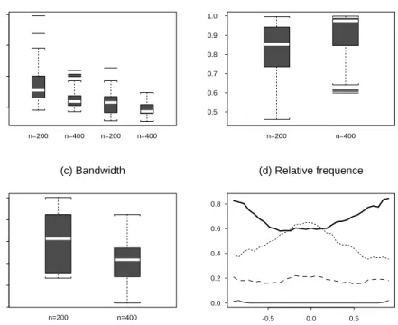
Figure1: SimulationresultsforExample1. (a)The boxplotsof themeanabsolutedeviationerror E

MAD

. The two panels on theleft are based on the estimated ,and the two panels on the right are basedon the true . (b)The boxplots of the absolute innerproduct j

T b

j. (c)The boxplots of selected bandwidths. (d)The plotsofthe relative frequencies ofdeletionof locally insignicant terms at z againstz: thinsolid line| fortheintercept; dotted line| forX

t1

,thicksolid line| forX

t2

,and dashed line|forX t3

.

Example 1. Letusconsidertheregression model

Y t = 3expf Z 2 t g+0:8Z t X t1 +1:5sin(Z t )X t3 +" t ; (5.2) with Z t = 1 3 (X t1 +2X t2 +2X t4 ); where X t (X t1 ;:::;X t4 ) T

, for t 1, are independent random vector uniformly distributed on

[ 1;1] 4

,and f" t

gisa sequenceofindependentstandardnormal randomvariables. It iseasyto see

thattheregressionfunctionintheabovemodelisintheformof(3.3)withd =4,= 1 3

(1;2;0;2) T

,

and thecoeÆcient functions

g 0 (z)=3e z 2 ; g 1 (z)=0:8z; g 2 (z)0; and g 3 (z) =1:5sin(z):

We nowapplythealgorithmdescribedinx3.2.5to estimateparametersinthismodel. We conduct

two simulationswith sample size200 and 400 respectively, each with 200 replications. The CPU

are summarized in Fig. 1. Fig. 1(a) displays the boxplots of the mean absolute deviation errors.

Wealsoplotthemeanabsolutedeviationerrorsobtainedusingthetruedirection. Thedeciency

due to unknown decreases when the sample size increases. Fig. 1(b) shows that the estimator b

derived fromthe one-stepiterative algorithm is closeto thetrue with highfrequencies inthe

simulationreplications. Theaverageiterationtimeinsearchforis14.43forn=400and18.25for

n=200. MostoutliersinFig.1(a)andFig.1(b)correspondtothecaseswherethesearchfordid

notconverge within30iterations,whichistheupperlimitsetinthesimulation. Fig.1(c)indicates

that theproposed bandwidthselector describedin x2.2.3 seems quite stable. We also appliedthe

methodinx2.2.4 to choosethelocalsignicant variablesat the31 regulargrid pointsintherange

from -1.5 to 1.5 times of thestandard deviationsof T

X. The relative frequencies of deletionare

depicted in Fig. 1(d). There is overwhelming evidence to include the `intercept' g 0

(z) =3e z

2 in

themodelforallthevaluesofz. Incontrast, wetendto deletemostoften thetermX t2

whichhas

`coeÆcient' g 2

(z)0. There isstrong evidence to keepthe termX t3

inthemodel. Note thatthe

termX t2

islesssignicant,themagnitudeof its`coeÆcient' g 1

(z)=0:8z beingsmaller thanthose

of bothg 0

(z) and g 3

(z).

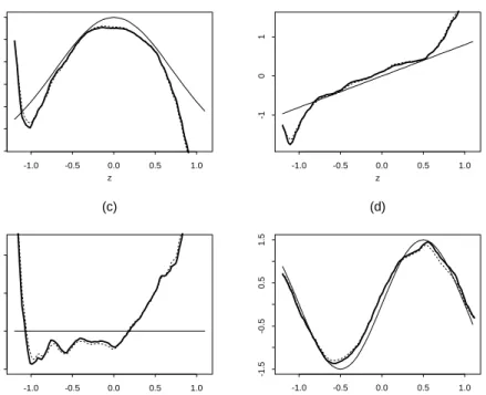
Fig. 2presentsa typicalexampleof theestimatedcoeÆcient functions. The curvesareplotted

on the range from -1.5 to 1.5 times of the standard deviation of T

X. The typical example

was selected in such a way that the corresponding E MAD

is equal to its median among the 200

replicated simulations withthe sample size n=400. For thisexample, the selected bandwidthis

0.597, T

b

= 0:946. For the sake of comparison, we also plot the estimated functions obtained

usingthetrue index. The deciencyduetounknown isalmostnegligibleonce b

isreasonably

accurate. Note thatthe biasesof estimatorsforthe coeÆcient functions g 0 ();g 1 () andg 2 () (but

notnecessarilyforg()) arelargenearto boundaries. We believethatthisisduetothecollinearity

ofvariablesX 1

;;X 4

andsmalleectivelocalsamplesizenearthetails. ThecoeÆcientfunctions

are notsoeasilyidentiedlocally inthose areas. However, there is no evidence that thisproblem

willdistorttheestimationforthetarget functiong(x).

Example 2. We nowconsidera timeseriesmodel

Y t = Y t 2 exp( Y 2 t 2 =2)+ 1 1+Y 2 t 2 cos(1:5Y t 2 )Y t 1 +" t ; (5.3) where f" t

gis a sequence of independent normalrandom variableswithmean 0 and variance0.25.

If we regard X t (Y t 1 ;Y t 2 ) T

as the regressor, (5.3) is of the form of model (3.3) with d = 2,

=(0;1), and g 0 (z)= zexp( z 2 =2); g 1 (z)=cos (1:5z)=(1+z 2 ):

Toillustratetheapplicationofouralgorithmtothismodel,weconducttwosimulationswithsample

size 200 and 400 respectivelywith 200 replications. For each replication, we predict the 50

post-sample pointsand compare them with thetrue values. One realizationwith samplesize 400 lasts

(a)

z

-1.0

-0.5

0.0

0.5

1.0

0.0

0.5

1.0

1.5

2.0

2.5

3.0

(b)

z

-1.0

-0.5

0.0

0.5

1.0

-1

0

1

(c)

z

-1.0

-0.5

0.0

0.5

1.0

-0.5

0.0

0.5

1.0

(d)

z

-1.0

-0.5

0.0

0.5

1.0

-1.5

-0.5

0.5

1.5

Figure 2: Simulationresults forExample1 (n =400). The plot of estimated coeÆcient functions (thick line), true functions (thin line), and estimated functions with true index (dotted line). (a)g 0 (z)=3e z 2 ;(b) g 1 (z)=0:8z; (c)g 2 (z)=0;(d)g 3 (z)=1:5sin(z).

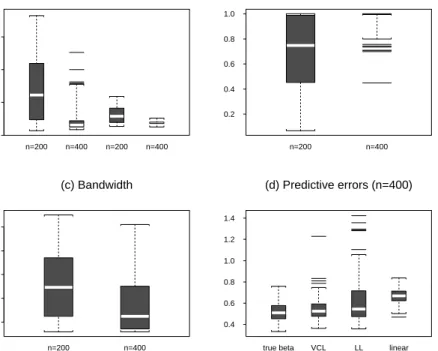
aPentiumII350MHzPC.TheresultsaresummarizedinFig.3. Fig.3(a)displaystheboxplots of

themeanabsolutedeviationerrors. Forsamplesizen=400,themediumsofE MAD

withestimated

and true areabout the same, although the distribution of E MAD

with b

hasa long tail on the

right. Fig.3(b) shows that the estimator b

derived from the one-step iterative algorithm is close

to the true with high frequencies in the simulation replications. The average iteration time in

search for is7.80 forn=400 and 17.62 forn=200. In fact, thesearchdid notconvergewithin

30 iterationsfor 21 out of 200 replications withn =200, and forone out of 200 replications with

n=400. Fig.3(c) is theboxplotof theselected bandwidths.

Wealso compared predictionperformanceofvariousmodelsinthesimulation withthesample

size n = 400. For each of 200 realizations, we predict 50 post-sample points from four dierent

models,namely thettedvarying-coeÆcientmodelswithtrue andestimated ,apurely

nonpara-metricmodel basedon locallinear regressionof Y t

on (Y t 1

;Y t 2

) withthebandwidthselected by

theGCV-criterion, and alinear autoregressive modelwith theorder (2) determinedbyAIC.In

oursimulation,AICalwaysselectedorder2inthe200replications. Fig.3(d)presentstheboxplots

of the average absolute predictive errors. The varying-coeÆcient models withtrue and estimated

arethetwo best predictorssincethey specifythecorrectform ofthetrue model(see Fig.3(d)).

Themedianofthepredictiveerrors fromthenonparametricmodelbasedonlocallinearregression

isaboutthesameasthatfromthevarying-coeÆcientmodel. Butthevarianceismuchlarger. The

Fig.4 presents a typical example of the estimated coeÆcient functions with the sample size

n=400. The curves are plottedon therange from -1.5 to 1.5 times of the standard deviation of

T

X. Forthecase withn=400, theselectedbandwidthis0.781, and T b =0:999. (Themedian of T b

inthesimulation of200 replications withn=400 is0.999.)

0.0

0.5

1.0

1.5

n=200

n=400

n=200

n=400

(a) Absolute deviation

0.2

0.4

0.6

0.8

1.0

n=200

n=400

(b) Inner product

0.5

1.0

1.5

2.0

2.5

n=200

n=400

(c) Bandwidth

0.4

0.6

0.8

1.0

1.2

1.4

true beta

VCL

LL

linear

(d) Predictive errors (n=400)

Figure3: SimulationresultsforExample2. The boxplotsof (a)themeanabsolutedeviationerror E

MAD

(the twopanelson theleftarebasedon b

,andthetwo panelsontherightarebased onthe true ), (b) the absolute inner product j

T b

j, (c) the selected bandwidths, and (d) the average absolutepredictiveerrorsofthevarying-coeÆcientmodelswithtrueand

b

,nonparametricmodel based onlocallinearregression, andlinear AR-modeldetermined byAIC(fromleft to right).

(a)

z

-1.5

-1.0

-0.5

0.0

0.5

1.0

1.5

-0.6

-0.4

-0.2

0.0

0.2

0.4

0.6

(b)

z

-1.5

-1.0

-0.5

0.0

0.5

1.0

1.5

-0.5

0.0

0.5

1.0

Figure4: SimulationresultsforExample2. TheplotofestimatedcoeÆcientfunctions(thickline), true functions (thin line). (a) g

0 (z) = ze z 2 =2 ; (b) g 1 (z) =cos (1:5z)=(1+z 2

). The sample size n=400.

Y t = 3exp ( Z 2 t +X t1 )+(Z t +X 2 t1 )X t1 log (Z 2 t +X 2 t1 )X t2 +1:5sin(Z t +X t1 )X t3 +" t ; withZ t = 1 2 (X t1 +X t2 +X t3 +X t4 ); wherefX t1 ;:::;X t4 gandf" t

garethesameasinExample1. Obviously,theregression functionin

theabovemodelisoftheform(4.1)withd=4,= 1 2 (1;1;1;1) T ,V t =X t1

andthetwo-dimensional

coeÆcient functions g 0 (z;v)=3e z 2 +v ; g 1 (z;v)=z+v 2 ; g 2 (z;v)= log (z 2 +v 2 ); g 3 (z;v)=1:5sin(z+v);

whichareplottedinFig.5. AssumingthedirectionofV t

=X t1

isgiven,wenowapplythealgorithm

described inx3.4 to estimate thecoeÆcient functions. We conduct three simulationswith sample

size200, 400 and 600 respectively,each with 100 replications. The CUPtime foreach realization,

inaSunUltra-10 300MHzWorkstation,isabout18 secondsforn=200, 1minuteand 20seconds

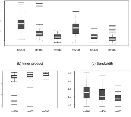
for n =400 and 3 minutes and 10 seconds for n = 600. Fig. 6(a) shows that the mean absolute

deviation errordecreaseswhen n increases. For thesake of comparison,we also presentthe mean

absolutedeviationerroroftheestimatorbasedontruevalueof. Fig.6(b)displaystheboxplotsof

theabsolute innerproductj T

b

j, whichindicates thatthe one-step iterationalgorithm described

inx3.2 worksreasonablywell. Theboxplotsof bandwidthsselected bytheGCV-methodstatedin

x3.3 aredepictedinFig. 6(c).

-1.5

-1

-0.5

0

0.5

1

1.5

z

-0.5

0

0.5

1

v

0

2

4

6

8

(a)

-1.5

-1

-0.5

0

0.5

1

1.5

z

-0.5

0

0.5

1

v

-2

-1

0

1

2

3

(b)

-1.5

-1

-0.5

0

0.5

1

1.5

z

-0.5

0

0.5

1

v

-2

0

2

4

6

8

(c)

-1.5

-1

-0.5

0

0.5

1

1.5

z

-0.5

0

0.5

1

v

-1.5

-1

-0.5

0

0.5

1

1.5

(d)

Figure 5: The coeÆcient functions of Example 3. (a) g 0 (z;v) = 3e z 2 +v , (b) g 1 (z;v) = z+v 2 , (c)g 2 (z;v)= log(z 2 +v 2 ),and (d)g 3 (z;v)=1:5sin(z+v).

0.6

0.8

1.0

1.2

1.4

n=200

n=400

n=600

n=200

n=400

n=600

(a) Absolute deviation

0.4

0.5

0.6

0.7

0.8

0.9

1.0

n=200

n=400

n=600

(b) Inner product

0.5

1.0

1.5

2.0

2.5

n=200

n=400

n=600

(c) Bandwidth

Figure 6: Thesimulationresults forExample3. The boxplots of (a) themean absolute deviation error E

MAD

, (b) the absolute inner product j T

b

j, and (c) the selected bandwidths. The three panelson theleftin(a)arebased onthe estimated,and thethree panelsontheright arebased on thetrue . Thethree panelson theleft in(a) arebased on theestimated ,and the three on theright arebased onthe true.

5.2 Real data examples

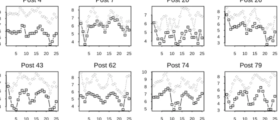
Example4. Theannualnumbersofmuskratsandminkcaughtover82trappingregionshavebeen

recentlyextractedfromthe recordscompiledbythe HudsonBayCompanyonfursalesat auction

in1925-1949. Fig. 7indicates the82 posts wherefurswerecollected. Biological evidence suggests

that mink is a key predator on muskrat (Errington, 1961, 1963). Fig. 7(b) plots the time series

of the mink and the muskrat (on the natural logarithmic scale) from 8 posts selected randomly

among the 82 posts. Most seriesexhibit cycles with a period of around 10 years. There exists a

clearsynchronybetweentheuctuationsofthetwospecieswithadelayofaboutone ortwoyears.

Since there is a general lackof data on bothprey and predator from thesame area and over the

same time period,this data set oers a unique opportunity for quantitative analysis aiming at a

deeperunderstandingof theinteractionbetweenprey(i.e. muskrat)and predator(i.e. mink). As

astartingpoint,weintroduceanecologicalmodelto describethemink-muskratinteraction. Based

(PutFig.7(a) here)

Post 4

5

10

15

20

25

4

5

6

7

8

9

Post 7

5

10

15

20

25

4

5

6

7

8

Post 20

5

10

15

20

25

4

5

6

7

Post 26

5

10

15

20

25

3

4

5

6

7

8

Post 43

5

10

15

20

25

4

5

6

7

8

Post 62

5

10

15

20

25

4

5

6

7

8

Post 74

5

10

15

20

25

5

6

7

8

9

10

Post 79

5

10

15

20

25

3

4

5

6

7

8

(b) Mink-muskrat time series from 8 posts

Figure7: (a) A mapof82 posts forthe minkand themuskrat inCanadain1925 {1949. (b)The timeseriesplots ofthemink and themuskrat datafrom 8 randomlyselected posts. Solidlines | mink;dashed lines| muskrats.

model to describethepredator-prey interaction,namely 8 < : X t+1 X t = a 0 ( t ) a 1 ( t )X t a 2 ( t )Y t ; Y t+1 Y t = b 0 ( t ) b 1 ( t )Y t +b 2 ( t )X t ; (5.4) where X t and Y t

denote the population abundances, on a natural logarithmic scale, of muskrat

and mink respectivelyat time t, a i

() and b i

() are non-negative functions, and t

is an indicator

representing the regime eect at time t, which is determined by X t

and/or Y t

. The term `regime

eect'collectivelyreferstothenonlineareectdueto,amongothers,thedierenthunting/escaping

behaviororthedierentreproductionratesofanimalsatdierentstages ofpopulationuctuation

(Stensethetal.,1999). Biologicallyspeaking, a 1 ( t )andb 1 ( t

)reectthewithinspeciesregulation

whereasa 2 ( t ) andb 2 ( t

)reectthefoodchaininteractionbetweenthetwospecies,anda 0 ( t )and b 0 ( t

) arethe intrinsicratesof changes. A simpleoptionwhich facilitates statisticaldata analysis

isto use athresholdvariable to denetheregime eect which switchesbetweentwo regimes. The

model implied,with addedrandomnoise,could have theform 8 < : X t+1 = (a 10 +a 11 X t +a 12 Y t )I(X t r 1 )+(a 20 +a 21 X t +a 22 Y t )I(X t >r 1 )+" 1;t+1 ; Y t+1 = (b 10 +b 11 Y t +b 12 X t )I(X t r 2 )+(b 20 +b 21 Y t +b 22 X t )I(X t >r 2 )+" 2;t+1 ; (5.5)

where we choose muskrat variable X t

as the threshold variable. It is easy to see from (5.4) that

botha 12

and a 22

shouldbe non-positive,andbothb 12

andb 22

shouldbe non-negative. The model

(5.5) assumesthepopulationsmuskrat andmink arepiecewiselinearfunctions oftheirimmediate

lagged values. Note that each time series has only 25 points, which imposes intrinsic diÆculties

for statistical data analysis even with simple nonlinear models such as (5.5). Yao et al. (1998)

and theother sixpostson itsrightinFig.7;thewesternareaconsistingofthe30 posts ontheleft

in Fig. 7 (i.e. post 17 and those on its left); and the centralarea consisting of theremaining 43

postsin themiddle. Yao etal. (1998) tted model (5.5) to each ofpooleddata sets and reported

some interesting andecologically interpretablendings.

(a) Mink model for central area

z

-1

0

1

-0.6

-0.4

-0.2

0.0

0.2

0.4

0.6

(b) Muskrat model for central area

z

-3

-2

-1

0

1

2

3

-1.0

-0.5

0.0

0.5

1.0

(c) Mink model for western area

z

-2

-1

0

1

2

-1.0

-0.5

0.0

0.5

1.0

(d) Muskrat model for western area

z

-1

0

1

2

-1.0

-0.5

0.0

0.5

1.0

(e) Mink model for eastern area

z

-1

0

1

-1.0

-0.5

0.0

0.5

1.0

1.5

(f) Muskrat model for eastern area

z

-2

-1

0

1

2

0.0

0.5

1.0

1.5

Figure 8: Estimated coeÆcient functions for Canadian mink-muskrat data. (a), (c) & (d): thick solid lines | g x (); solid lines | g y (); dashed lines | g 0

(). (b), (d) & (f): thick solid lines | f y (); solidlines| f x ();dashed lines| f 0 ().

Clearly,themodel(5.5)simpliesthenonlinearinteractioninto twostates(foreach ofmuskrat

or mink models) with a prescribed threshold variable X t . Note that X t X t 1 is the muskrat

population growth rate. It is biologically interesting to nd out which would be an appropriate

`threshold'variable to denethe regime eect among X t ,X t X t 1 ,Y t and Y t Y t 1 . Withthe

8 < : X t+1 = f 0 (Z t )+f 1 (Z t )Y t 1 +f 2 (Z t )Y t +f 3 (Z t )X t 1 +" 1;t+1 ; Y t+1 = g 0 (Z t )+g 1 (Z t )Y t 1 +g 2 (Z t )Y t +g 3 (Z t )X t 1 +" 2;t+1 ; (5.6) whereZ t = 1 Y t 1 + 2 Y t + 3 X t 1 + 4 X t with( 1 ; 2 ; 3 ; 4 ) T

selected bydata. Comparing

with(5.4)and(5.5),weincludefurtherlaggedvaluesX t 1

and Y t 1

intotheabovemodel. We will

applythelocalvariableselectiontechniqueinx2.2.4todetectanyredundantvariablesat31regular

gridpointsovertherangefrom-1.5to1.5timesofstandarddeviationofZ t

. Toeliminatetheeect

ofdierentsamplingweightsindierentregionsand fordierent species,we rststandardizedthe

mink series and muskrat series separately for each post. Since there are some missing values in

the data from post 15, we exclude it from our analysis. The sample size for eastern, central and

western areas aretherefore 207,989 and 667 respectively. Wedenote R MSE

theratioof themean

squareserrors fromthetted model over thesample variance ofthevariable to betted.

First,weusethesecondequationof(5.6)tomodelminkpopulationdynamicsinthecentralarea.

Theselected is(0:424;0:320;0:43 2;0:7 33 ) T

,theselected bandwidthis0.415, andR MSE

=0:449.

The local variable selection indicates that X t 1

is the least signicant variable over all, for it is

signicant at only7outof 31 grid points;see x2.2.4. Byleavingitout, we reduce to themodel

Y t+1 =g 0 (Z t )+g y (Z t )Y t +g x (Z t )X t +" 2;t+1 ; (5.7) whereZ t = 1 Y t + 2 X t + 3 Y t 1

. Our algorithm selected

Z t =(0:540Y t 0:634Y t 1 )+0:553X t ; (5.8)

which suggests that thenonlinearityis dominatedbythegrowth rateof mink and thepopulation

of muskrat inthe previousyear. The estimated coeÆcient functions are plottedin Fig.8(a). The

coeÆcient function g x

() is positive, which reects the fact that a large muskrat population will

facilitate the growth of the mink population. The coeÆcient function g y

() is also positive, which

indicatesanaturalreproductionprocessofminkpopulation. Bothg y

()andg x

()areapproximately

increasingwithrespecttothesumofgrowthrateofminkandpopulationofmuskrat;see(5.8). But

the`intercept' g 0

() drops sharplyafterZ t

reaches athresholdaround 1. This mightbe relatedto

thefact that mink populationcould suer from its over-sizedgrowth rate dueto the competition

for food and living environment among mink themselves. All the terms in the model (5.7) are

signicant inmost places; the number of signicant grid points for `intercept', Y t

and X t

are 21,

31 and 26(out of 31intotal). The selected bandwidthis0.597 and R MSE

=0:461.

Fitting the rst equation of (5.6) to muskrat dynamics in the central area, we obtained b = (0:632;0:308;0:21 0;0:6 80 ) T , b h=0:346 and R MSE

=0:518. The overall least signicantvariable is

Y t 1

whichis onlysignicantin 9outof 31 grid points. By leave itout, themodelisreducedto

X t+1 =f 0 (Z t )+f y (Z t )Y t +f x (Z t )X t +" 1;t+1 ; (5.9) whereZ t = 1 Y t + 2 X t + 3 X t 1

. Theresultsfromttingareasfollows: Z t =0:542Y t +0:720X t + 0:435X t 1 , b h=0:498 andR MSE

coeÆcient functionf y

()isalwaysnegative,whichreectsthefactthatminkisthekeypredatorof

muskratinthiscoreoftheborealforestinCanada. ThecoeÆcientf x

()ispositive,aswell-expected.

Werepeatedtheaboveexerciseforpooleddatainthewesternarea,andobtainedsimilarresults.

In fact, the model (5.7) appears appropriate for mink dynamics with Z t = 0:469Y t +0:723X t + 0:507Y t 1 , R MSE =0:446, b

h =0:415, and theestimated coeÆcient functions plotted inFig. 8(c).

Themodel(5.9)appearsappropriateformuskratdynamicswithZ t =0:419Y t +0:708X t +0:569X t 1 , b h=0:415, R MSE

=0:416, andthe estimatedcoeÆcient functionsplottedin Fig.8(d).

Finally,we tthedataintheeasternarea. Theresultsareradicallydierentfromthose ofthe

central and the west stated above. To t the mink dynamics with the second equation of (5.6),

we discovered that both X t

and X t 1

are signicant only in smallportions of the sample space.

After leavingoutX t 1

, the ttingwiththe model (5.7) give Z t =0:173Y t 0:394X t +0:901Y t 1 , b h = 0:597 and R MSE

= 0:681. The local variable selection indicates that out of 31 grid points,

the `intercept', Y t

and X t

are signicant at 15, 31 and 4 points respectively. There is clear

auto-dependenceinminkseriesfY t

gwhilemuskratdatafX t

gcarry littleinformationaboutmink. The

estimatedcoeÆcients, depictedinFig.8(e),areconsistentwiththeaboveobservations. Thetting

ofthemuskratdynamicsshowsagainthatthereseemslittleinteractionbetweenminkandmuskrat

inthisarea. Forexample, thetermY t

inthemodel(5.9) isnotsignicantat allthe31 gridpoints

tested. The estimated coeÆcient functionf y

() is plottedas thethick curve inFig. 8(f), which is

alwaysclose to 0. We t thedatawitha furthersimpliedmodel

X t+1 =f 0 (Z t )+f x (Z t )X t +" 1;t+1 :

Theresultsareasfollows: Z t =0:667X t 0:745X t 1 , b h=0:498andR MSE =0:584. Theestimated

coeÆcient functions are superimposed on Fig. 8(f). Note thedierent rangesof z-values are due

to dierent Z 0 t

s areused intheabove modeland themodel (5.9).

Insummary,wehavefacilitatedthedataanalysisofthebiologicalfoodchaininteractionmodel

ofStensethetal. (1997) byportrayingthenonlinearitythroughvarying-coeÆcientfunctions. The

selection of the index inour algorithm is equivalent in this context to the selection of the regime

eect indicator, which in itself is of biological interest. The numerical results indicatethat there

is a strong evidence of predator-prey interaction between mink and muskrat in the central and

western areas. However, no evidence forsuch an interactionexists inthe easternarea. In light of

what isknownintheeasternarea,thisisnotsurprising. Thereisalargerarrayof prey-speciesfor

the mink to feedon, making it less dependent on muskrat. It has been also observed that foxes

have amuch more pronouncedinuenceon theentiresystem ofthisarea (Elton,1942).

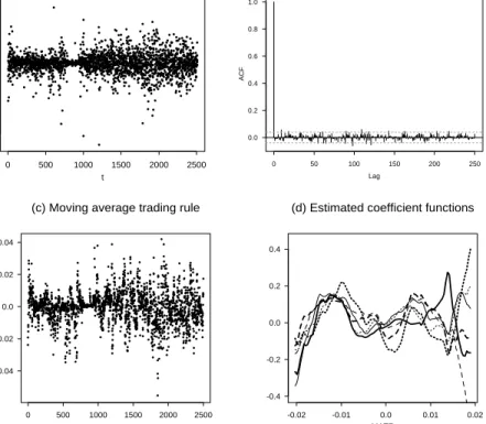
Example 5. This exampleconcerns thedaily closing bidprices of thepoundsterling interms of

USdollarfrom2January1974to30December1983,whichformsatimeseriesoflength2510. The

previousanalysisofthis`particularlydiÆcult'datasetcanbefoundinGallant,HsiehandTauchen

(1991) and the references within. Let X t