Porto Institutional Repository
[Doctoral thesis] Simplicial Data Analysis: theory, practice, and algorithms
Original Citation:
Alice, Patania (2017).Simplicial Data Analysis: theory, practice, and algorithms. PhD thesis Availability:
This version is available at :http://porto.polito.it/2670783/since: May 2017 Published version:
DOI:10.6092/polito/porto/2670783 Terms of use:
This article is made available under terms and conditions applicable to Open Access Policy Article ("Public - All rights reserved") , as described athttp://porto.polito.it/terms_and_conditions. html
Porto, the institutional repository of the Politecnico di Torino, is provided by the University Library and the IT-Services. The aim is to enable open access to all the world. Pleaseshare with ushow this access benefits you. Your story matters.
Doctoral Program in Mathematics (29 cycle)
Simplicial Data Analysis
theory, practice and algorithms
By
Alice Patania
******
Supervisor(s):
Prof. Francesco Vaccarino, Supervisor Dott. Giovanni Petri, Co-Supervisor
Doctoral Examination Committee:
Prof. Ginestra Bianconi , Referee, Queen Mary University of London, U.K. Prof. Annalisa Marzuoli, Referee, Universitá di Pavia, Italy
Prof. Federica Galluzzi, Universitá di Torino, Italy Prof. Gianfranco Casnati, Politecnico di Torino, Italy Prof. Emilio Musso, Politecnico di Torino, Italy
Politecnico di Torino 2017
I hereby declare that, the contents and organization of this dissertation consti-tute my own original work and does not compromise in any way the rights of third parties, including those relating to the security of personal data.
Alice Patania 2017
* This dissertation is presented in partial fulfillment of the requirements for
I strongly believe that there is no way that I would have made it to this point without fantastic people that dedicated their time and expertise to make me the researcher I am today.
Before I start a little disclaimer for all of you that supported me emotionally during these parst 4 years. I will pour my heart out to you at the end of this thesis. For now, allow me to thank the individuals without whose help and dedication this work would have never been written.
First and foremost, I cannot thank enough my supervisors Prof. Vaccarino and Dott. Petri, for their continuous support and constructive critique. They have encouraged me to take chances with my research and gave me countless opportunities which made me grow not only as a scientist, but as a pers on. Thank you, your advice on both research as well as on my career have been priceless. I would also like to thank my collaborators: Jean-Gabriel Young, Prof. Lloyd, Dott. Rebentrost for their invaluable assistance. Applying mathematical methods in so many different fields can be challenging, and their support was fundamental for the success of my work. I would like to thank the I.S.I. Foundation and the project S3: "Steering Socio-technical Systems" from Compagnia di San Paolo who financed my Ph.D. Fellowship and have given me so many fantastic opportunities, enabling me to carry out my research without any financial worry. I am eternally grateful to Prof. Mario Rasetti and the I.S.I. Foundation for the fantastic environment they were able to create, surrounding myself by absolutely fantastic people who have made the last four years completely splendid. I want to thank all the researchers that have been part of the I.S.I. family during my time there. You have all been a tremendous inspiration, and i will always be grateful for all the fun we have had in the
last four years. Lastly, I would like to acknowledge the valuable comments and suggestions of the reviewers, which have improved the quality of this thesis.
Simplicial complexes store in discrete form key information on a topological space, and have been used in mathematics to introduce combinatorial and discrete tools in geometry and topology. They represent a topological space as a collection of ‘simple elements’ (such as vertices, edges, triangles, tetrahedra, and more general simplices) that are glued to each other in a structured manner. In the last 20 years, they have been a basic tool in computer visualization and topological data analysis. Topological data analysis has been used mainly as a qualitative method, the problem being the lack of proper tools to perform effective statistical analysis. Coming from well established techniques in random graph theory, the first models for random simplicial complexes have been introduced in recent years, none of which though can be used effectively in a quantitative analysis of data. We introduce a random model which fixes the size distribution of facets and can be successfully used as a null model. Another challenge is to successfully identify a simplicial complex which can correctly encode the topological space from which the initial data set is sampled from. The most common solution is to build nesting simplicial complexes, and study the evolution of their features. A recent study uncovered that the problem can reside in making wrong assumption on the space of data. We propose a categorical reasoning which enlightens the cause leading to these misconceptions. The construction of the appropriate simplicial complex is not the only obstacle one faces when applying topological methods to real data. Available algorithms for homological features extraction have a memory and time complexity which scales exponentially on the number of simplices, making these techniques not suitable for the analysis of ‘big data’. We propose a quantum algorithm which is able to track in logaritmic time the evolution of a quantum version of well known homogical features along a filtration of simplicial complexes.
Introduction 1
1 Simplicial Complexes in Data Analysis 6
1.1 Abstract simplicial complex . . . 7
1.2 Constructing Simplicial Complexes from data . . . 11
1.2.1 Metric case . . . 12
1.2.2 Non-metric case . . . 16
1.3 Random simplicial complexes . . . 18
1.3.1 Generative models . . . 19
1.3.2 Descriptive models . . . 25
2 Simplicial Configuration Model 28 2.1 Configuration model for pure simplicial complexes . . . 28
2.2 Simplicial configuration model . . . 33
2.2.1 Correctness of the model . . . 34
2.2.2 Empirical results . . . 38
2.3 Generating random simplicial complexes . . . 44
2.3.1 Constraints on the sequences . . . 44
2.4 Future work . . . 49
3 Weighted graphs and P-Persistent homology 52
3.1 Basic Notions . . . 54
3.1.1 The category of topological spaces . . . 54
3.1.2 The category of simplicial complexes . . . 57
3.1.3 The categories of graphs . . . 58
3.2 P-weighted graphs and P-persistent objects . . . 60
3.2.1 Equivalence . . . 61
3.2.2 Adjunctions . . . 63
3.3 Application to homology: multi-persistent homology . . . 69
3.3.1 Considerations on topological strata . . . 75
3.3.2 Conclusions . . . 77
4 Quantum algorithm for persistent homology 78 4.1 Persistent Homology . . . 80
4.1.1 Expliciting homology maps . . . 81
4.2 Quantum construction of a simplicial complex . . . 84
4.2.1 Quantum notation . . . 84
4.2.2 Simplex quantum state . . . 85
4.3 Quantum algorithm for persistent homology . . . 88
Conclusions 93
References 96
[...]a theory that does not lead to the solution of concrete and interesting problems is not worth having. Conversely, any really deep problem tends to stimulate the development of theory for its solution.
Sir Michael Atiyah, Advice to a Young Mathematician
Throughout history, mathematics has been providing a language capable of making difficult problems understandable and manageable, and for these reasons it has become an efficient source of concepts and tools constituing the backbone of all scientific disciplines. Moreover abstract concepts from logic, algebra, and geometry have found new concrete use with the advent of the computer and the birth of programming. In this thesis we are going to focus on the application to computer science of one of the most versatile algebraic tools of the last centuries: the simplicial complex. Simplicial complexes were first introduced in 1895 by Poincaré in his seminal work "Analysis Situs" [87] as a simplicial decomposition (triangulation) of a manifold, and they are now not only a fundamental construction in combinatorial topology, but also the secret behind every 3D rendering and image recognition software [59, 90].
Simplicial complexes are elementary objects built from such simple polyhedra as points, line segments, triangles, tetrahedra, and their higher dimensional analogues glued together along their faces. Since the late 1800s they have been used to store in discrete form key information on a topological space and
to transform complicated topological problems into more familiar algebraic ones with the introduction of simplicial homology (we refer to Aleksandrov [2] for a beautiful account on the birth of combinatorial topology). Their use in computer science has changed drastically with the advent of Topological Data Analysis [41–43, 38, 21, 19, 20], which uses techniques from computational and algebraic topology to extract information from high-dimension, incomplete and noisy data-sets.
In this work we are going to focus on the theory (chapter 3), practice (chapter 2) and algorithms (chapter 4) of the application of simplicial complexes to data analysis. For each aspect, we are going to introduce original results and insights which are able to shade light on underdeveloped applications for TDA, and further advance the available tool set.
Outline of the thesis
The main intuition of TDA is that data is sampled from a topological space, and the shape of this space is important to better understand the data. To study the shape of the underlying space of data, TDA methods aim to construct a simplicial complex or a filtration of simplicial complexes from the original data, which encodes information on the shape of the underlying space. In Chapter 1 we define the concept of a simplicial complex, and introduce the basic mathematical constructions of simplicial complexes. We then proceed to survey the most suitable methods of construction, distinguishing if the data set can be considered sampled from a metric, or a non-metric space. These topological tools allow for a new type of explorative analysis of data which is able to reveal structures that were unobtainable through other approaches. The
field of topological data analysis has been growing rapidly in the last fifteen years, and its applications have led to discoveries in various fields: genomics [76, 83], sensor analysis [31, 30, 29, 47], brain connectomics [48, 49], fMRI data [84, 65], network science [85, 86], just to name a few.
With the increasing popularity of topological analysis it has become nec-essary to build sounder statistical foundations. Therefore, the first original contribution in this thesis is to develop a null model1 of simplicial complexes
capable of differentiating between meaningful results and random noise. In re-cent years, researchers have introduced the first proposals for random simplicial complexes coming from well established techniques in random graph theory: the Erdös-Renyi random graph model [61, 67, 55, 62, 56, 57, 27], preferential attachment [13–15], the exponential random graph model [96], configuration model [28, 94]. Even though these models are good for theoretical studies, they present some shortcomings when used as null models of real data sets, which we present extensively in chapter 1 before introducing in chapter 2 the first original contribution of this thesis: the simplicial configuration model.
The simplicial configuration model builds on the work by Courtney and Bianconi [28] where the authors introduced a configuration model for simplicial complexes, which uses the intuition that the one-mode projection of a bipartite graph can be encoded as a simplicial complex. In their paper, Courtney and Bianconi analyzed in detail the ensemble of the configuration model for simplicial complexes with constant facet size. Our contribution generalizes their approach to general simplicial complexes. Moreover, we show how our
1In this context, by null model we mean an instance of a random simplicial complex which
random generative model can be used successfully as a null model for the size distribution of maximal facets in a general simplicial complex.
It is easy to see how the analysis we just introduced are significative if and only if we can safely assume that the starting simplicial complex successfully incorporates the features of the dataset. However, there is seldom a way to un-equivocally test whether a simplicial complex correctly encodes the topological space from which the initial data set is sampled from. For this reason, the most common approach is to build nesting simplicial complexes from the data set, and study the evolution of their features across the filtration [42, 43, 38, 19]. This technique is known as persistent homology, and in recent years has become one of the prominent tools in TDA.
Following the example of many researchers [17], that in recent years worked on using category theory to build a stronger foundation for topological data analysis and highlighten its faults, in chapter 3 we start exploring the concept of persistence, and prove the adjuctions and categorical equivalences that dictate the relationships between the categories involved in topological data analysis (topological spaces, graphs, simplicial complexes) [78]. We show how these results dissuade from using the intrinsic metric of graphs (shortest path length metric) for constructing simplicial complexes, backing the empirical results in [86].
In the last chapter of this thesis, we dive into the computational problems that might arise when applying these methods to real data. In fact, the construction of an appropriate simplicial complex is not the only obstacle one faces when applying topological methods to real data. Available algorithms for homological features extraction have a memory and time complexity which
scales exponentially on the number of simplices, making these techniques not suitable for the analysis of ’big data’. With an eye to this problem, we formulated an approach based on quantum computation [81]. Expanding on a method by Lloyd et al. [63], we propose a quantum algorithm which is able to track in logarithmic time the evolution of a quantum version of well known homological features along a filtration of simplicial complexes.
Simplicial Complexes in Data
Analysis
In this chapter we introduce some basic notions from classical algebraic topology that are widely used in topological data analysis. We define the most common types of simplicial complexes (sec. 1.1), and how to construct them from data (sec. 1.2). Finally in section 1.3 we give a thorough introduction to existing
models for random simplicial complexes.
Unless otherwise stated, we consider to be working on a field k, that we
sup-pose to be algebraically closed. Moreover, we supsup-pose all the algebras to be associative and all the modules to be left module if not otherwise specified.
1.1
Abstract simplicial complex
Simplicial complexes are one of the most intuitive concepts in mathematics. They are built from such simple polyhedra as points, line segments, triangles, tetrahedra, and their higher dimensional analogues glued together along their faces. Even if their intuition is very geometric, they can easily be generalized to abstract mathematical objects. Anabstract simplicial complex X is a
collection of finite sets such that for every σ ∈ X then for all τ ⊆σ, τ ∈ X.
The sets in X are called simplices, the dimension of a simplex σ ∈ X is
dim(σ) =card(σ)−1; the dimension of X is the maximum dimension of the
simplices it contains.
The proper subsets of a simplex are called its faces and, if τ is a proper face
of σ, then σ is a proper coface of τ. A facet is any simplex in a simplicial
complex that is not a face of any other simplex. A simplicial complex is called
pureif all its facets have the same dimension. The vertex set ofX is the union
of all the simplices it contains, V =∪σ∈Xσ.
Examples of abstract simplicial complexes
We now introduce some concepts related to simplicial complexes which will be useful in the future chapters.
Subcomplex AsubcomplexX′ ofXis an abstract simplicial complex such
that the vertex set of X′ is contained in the vertex set of X, and, for every
simplex σ inX′,σ belongs to X as well. An important type of subcomplex is
of dimension at most k in X, X(k) = {σ|dimσ ≤ k}. In particular, the 1
-skeleton of a simplicial complex can be considered as an undirected graph, since it contains only 1-simplices (edges) and 0-simplices (vertices); from this moment onward we will then refer to X(1) as the underlying graph of X. It
is easy to see how the 1-simplices and 0-simplices contained in any simplex in
X, form cliques (complete subgraphs) inX(1). Beware that the opposite it is
not necessary true, that is, a clique in the underlying graph of X is not always
a representation of a simplex in X. The simplicial complexes for which this
property is verified are called flag complexes.
Clique complex It is easy to see how to use this definition to construct flag
complexes from graphs. Given a graph G, the clique complexCl(G) is the
simplicial complex whose simplices are all the cliques contained in G. A set
of vertices S ∈ V(G) of a graph is said to be independent, if for all v, w∈S
the edge (v, w)∈/ E(G). It is easy to see that the independent sets of G are
the cliques in the graph complement of G, i.e. the graph that has the same
vertices as Gand all the edges (v, w)such that (v, w)∈/ G. The independent complexInd(G)of a graph Gis the clique complex of the graph complement
of G.
Simplicial complex subdivisions The simplicial complexes we introduced
above are used in practice to describe the structural composition of the original simplicial complex. There might be the need in practice to construct a simplicial complex which has the same geometry and topology of the original one, but with a finer resolution. That is, a simplicial complex which contains all the simplices of the original one. A simple example of such a construction is the
stellar subdivision. Let σ be a simplex of X, the stellar subdivision of
X at σ is the abstract simplicial complex SdX(σ), where the set of vertices
V(SdX(σ)) =V(X)∪σˆ whereσˆ is the new vertex indexed byσ. Ifσ is already
a vertex we have thatσˆ =σ and no new vertex is introduced. Every simplex
that does not contain σ as a subset is still a simplex in SdX(σ). Otherwise, if
a simplex τ in X containsσ as a subset then η∪ {σˆ} ∈SdX(σ), where η is the
difference as sets between τ and σ.
The stellar subdivision is a construction which acts locally on the simplices that contain σ. A global construction of a finer complex is the barycentric
subdivision. The barycentric subdivision of X is an abstract simplicial
complex Bd(X), where the set of vertices in Bd(X) is indexed by the non
empty simplices inX, and
Bd(X) ={{σ1, . . . , σt}|σ1 ⊃ · · · ⊃σt, σi ∈X, t≥1} ∪ {∅} (1.1.1)
It is easy to observe that Bd(X) is a flag complex.
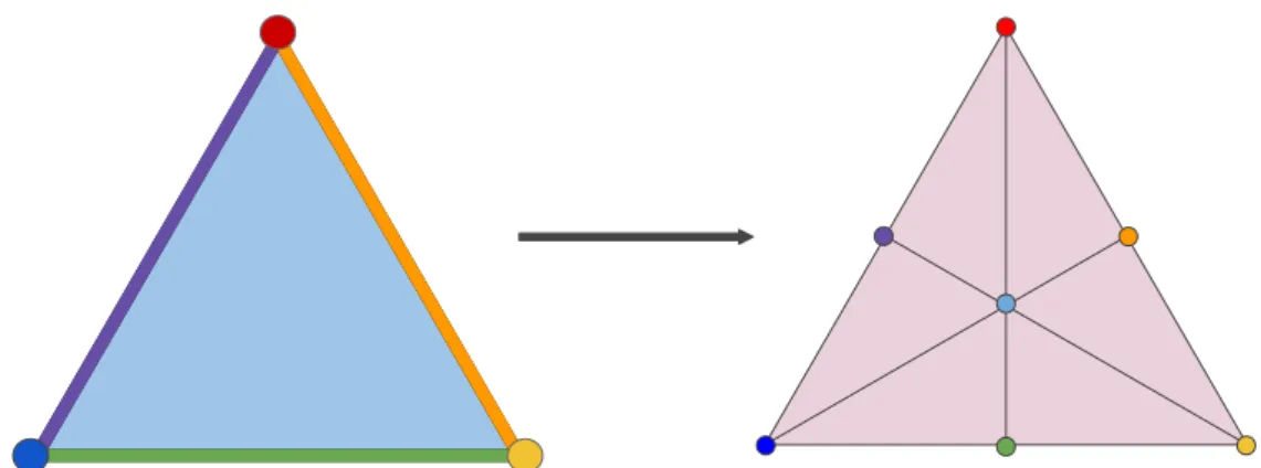
Fig. 1.1 Baricentric subdivision of a 2-simplex.
A typical application of this refinement process is in 3D imagining, when trying to increase the level of details in a picture. It can be proved that
taking the barycentric subdivision can be accomplished by a sequence of stellar subdivisions, which are performed locally and thus provide a computationally more economic construction.
Order Complex A partial ordered set, or poset, is a set P endowed with a
binary relation ≤ which is reflexive (for all a∈P,a ≤a), antisymmetric (for
all a, b∈P, if a≤b and b ≤a then a=b), and transitive (for alla, b, c∈P,if a≤ b and b ≤ cthen a ≤c). An abstract simplicial complex X can then be
considered a poset, since the inclusion of simplices is a partial order relation on
X. One can also construct a simplicial complex from any poset P, considering
as simplices all finite chains (i.e. finite totally ordered subsets) of P. The
simplicial complex defined in this way is calledorder complexofP. To better
clarify the concept, we give some examples of order complexes:
1. The order complex of a totally ordered set A is a simplex ∆(A).
2. Let n∈N and let Bn be the set of all subsets of n partially ordered by
inclusion. One can see that the order complex ∆(Bn) is isomorphic to
the barycentric subdivision of an (n−1)-simplex.
3. An abstract simplicial complex X can then be considered a poset, since
the inclusion of simplices is a partial order relation on X. Then, the
barycentric subdivision of X is the order complex of X considered as a
poset.
In chapter 3 we will go in more detail on the key role the order complex plays when analysing data with topological methods.
1.2
Constructing Simplicial Complexes from data
There are two main applications for simplicial complexes in data analysis: the representation of relations, and the discretization of data spaces. In the former, representing relational data, the vertices of the complex are the data points and ak−simplex represents a relation between the k+ 1vertices it contains.
In this application, the structure of the simplicial complex comes directly from the dataset itself. In the latter, objects are a topological discretization of the underlying space of data, that is, an object that is topological equivalent to the space from which we sampled the data.
In this section we will show some common simplicial complexes constructed from point clouds, distinguishing the cases in which the dataset is supposed to be sampled from a metric space and those in which it is not.
Before going on with the explanation, we introduce the nerve of an open cover, a construction at the core of the techniques we are going to describe in this section. Let X be a paracompact topological space, that is a topological
space in which to every open coverU one can associate a new coverV ofX with
a locally finite index set, such that every set inV is contained in some set in U. To each open cover U ={Uα}α∈A of X, we can associate an abstract simplicial
complex N(U) called the nerve of U. The simplicial complex is constructed in the following way: there is a vertex vα for each open set Uα in cover. A set
of k+ 1 vertices spans a k-simplex whenever the k + 1 corresponding open
sets Uα have non empty intersection. Obviously the simplicial complex thus
The following theorem gives the motivation for which the nerve is such a common tool for constructing simplicial complexes from data. Under appro-priate hypothesis, the nerve of and open cover has the same homotopy as the underlying topological space, that is, intuitively, it has the same "shape".
Theorem 1.2.1 (Nerve Theorem,[Hatcher, §4G.3]). Let X be a topological
space and U ={Uα}α∈A a countable open cover of X.
If, for every ∅ ̸= S ⊆ A, ∩s∈SUs is contractible or empty then N(U) is
homotopically equivalent to X.
1.2.1
Metric case
In applications it is quite common to work with large sets of points sampled from a metric space X. For example, to scan surfaces in 3D one uses
time-of-flight cameras which compute the nearest point on the surface from the sensor position along a given direction. A 3D scan may then be composed by a very large set of points corresponding to different directions from the sensor and different sensor positions.
In this section we will consider the data points as sampled from a metric space (X, m), where m is a metric, bestowed with the standard topology where
the baseB is made of open balls of radiusε centered in v ∈X,B= {Bε(v)|ε∈
R+, v ∈X} where Bε(v) ={u∈X|m(u, v)< ε}.
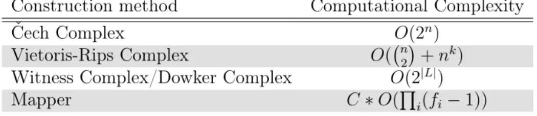
Čech Complex The Čech Complex is the nerve of an open covering of the
data set where the open sets are open balls Bε(v)of radius ε centred in v ∈X.
If we denote V as the set of v ∈ X such that Bε(v) ∈ U then we can write
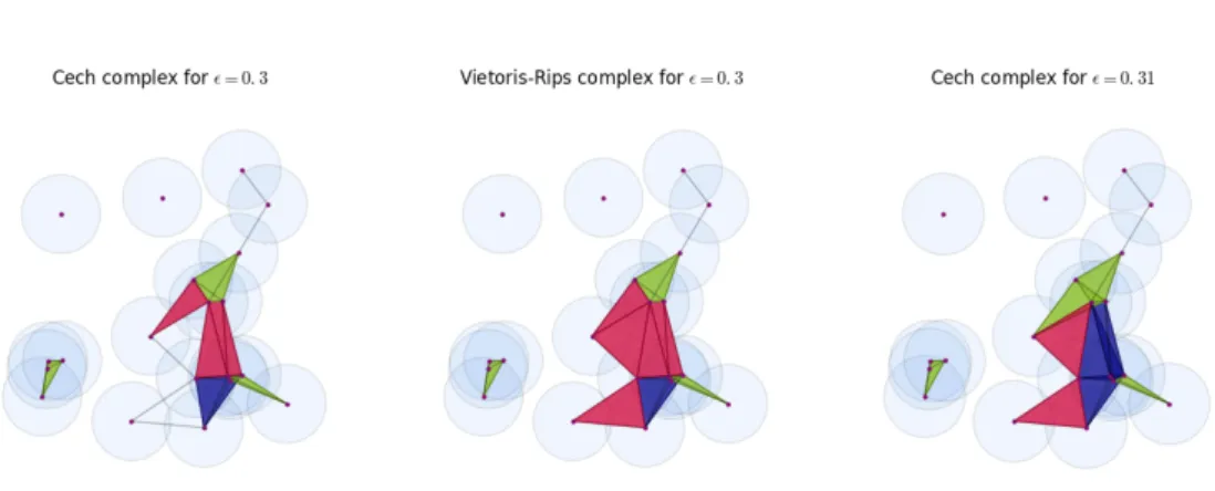
Fig. 1.2 A vizualization of the relation between Čech and Vietoris Rips at different scales described by proposition 1.2.2.
is called Čech complex Cˇ(V, ε). More concretely, the vertices of the Čech
complex are the points inV andk+ 1points spans ak-simplex if all theε-balls
centred in them have non-empty intersection. Since open balls are contractible, from Theorem 1.2.1 follows that the Čech complex captures the topology of the covering.
It is important to notice though that the resulting shape of the covering, and thus that of the Čech complex, depends on the choice of the radius of the open balls that form the covering. When the parameter is very small, smaller than the minimum distance between the points, the corresponding Čech complex is only composed by the points of V. Conversely, when the parameter value
is larger than the cloud diameter the corresponding complex contains all the possible subsets of V. The supposition here is that for a parameterε¯the open
cover of the dataset is also and open cover of the space X underlying the data
satisfying 1.2.1. Finding the optimal radiusε for which this happens is very
difficult. In recent years, new methods in topological data analysis have been introduced to avoid taking this decision, which we will look at in detail in Chapter 3.
Vietoris-Rips complex The Čech complex is a very good discretization of
the space X, but it is rarely used in practice because it is computationally
heavy to construct. This is due to the fact that its construction requires the computation of2|A| intersections, where |A| is the number of open sets in the
considered cover, which is equal to the number of vertices. Even though the computational complexity can be reduced with clever algorithms, the process is still a very expensive one. This is why less precise but more computational efficient simplicial complexes were introduced.
The Vietoris-Rips complex is popular in topological analysis thanks to the ease of its construction in every dimension. It is not a nerve as the other previously presented complexes, but it is the clique complex of a particular graph. Let X be a metric space with metric d, a Vietoris-Rips complex
V R(X, ε) is the simplicial complex which has as vertex setX and such that
{x0, . . . , xk}spans ak-simplex if and only if d(xi, xj)≤εfor all0≤(i−j)≤k.
Proposition 1.2.2 ([60]). Let X be a metric space with metricd, the following inclusions are satisfied :
ˇ
C(X, ε)⊆V R(X,2ε)⊆Cˇ(C,2ε) (1.2.1)
This proposition justifies the use of the Vietoris-Rips complex as a good-enough substitute of the Čech Complex. Applying this technique solves the computational problems, since it only requires to check if the distances are below a certain threshold for each pair of data points, and there are n
2
such matchings.
Witness complexes The methods introduced above produce simplicial
com-plexes whose vertex set has the same size as the underlying set of point cloud data. When working with big data sets, these constructions produce simplicial complexes which are untreatable. In 2004 De Silva and Carlsson, using ideas motivated by the usual Delaunay complex in Euclidean space, introduced a new method [29], the witness complex, which produces topologically equivalent simplicial complexes with a smaller vertex set.
Let X be a metric space, ε >0 a parameter and lets suppose we have a
finite subsetL ⊆X that we denote aslandmark set. For everyx∈X let mx
be the minimum distance between xand the set L, we shall define the strong witness complex as the complex Ws(X,L, ε)which has as vertex set L and
{l0, . . . , lk} spans a k simplex if and only if there existsx∈X (called witness)
such thatd(x, li)≤mx+ε ∀i.
This definition is too constraining creating a very small set of strong witnesses, in order to obtain a finer simplicial complex a weaker version of this construction was introduced. Let X be a topological space, point setL ⊆ X,
Λ ={l0, . . . , lk}finite subset of L. Thenx∈X is called aweak witness for
Λ, if for all i = 0, . . . , k, d(x, l)≥d(x, li) for all l ∈ L\Λ. Moreover for ε≥ 0
we will say that x is an ε-weak witness for Λ if d(x, l) +ε ≥ d(x, li) for all
i= 0, . . . , k and l ∈ L\Λ.
We can now construct the weak witness complex Ww(X,L, ε) and we
will say that Λ ={l0, . . . , lk}spans a k-simplex if and only ifΛ and all its faces
have a weakness ε. This complex depends on the choice of the landmark set.
There is no preferred way to choose an optimal landmark set. It is common practice to work with different set of landmarks and see if the results are
replicable. It is however one of the most popular constructions when working with large data sets since it contains a less simplices than the Vietoris-Rips complex, but it is as reliable in approximating the topology of the space.
1.2.2
Non-metric case
Depending on the data set we are working on, it is not always straight forward to know what metric the underlying space has, or whether a metric exists at all. In applications, we rarely have the certainty that the underlying space is a metric space. This is the reason why we introduce now two methods for constructing simplicial complexes which do not require the existence of a metric.
Dowker Complex The Dowker complex was first introduced in [24] and
named after C. H. Dowker [34] who compared two simplicial complexes con-structed from a binary relation. It is defined as follows: let L, W be two sets
and Λ :L×W →R be a function. Fora∈R consider the simplicial complex Dow(Λ, a) with vertex set Land simplices σ determined by:
∃ w∈W such that Λ(l, w)≤a for all l ∈σ (1.2.2)
Remark 1.2.2.1. The simplicial complexes introduced in Subsection 1.2.1 can all
be considered as examples of Dowker Complex where as functionΛis considered
the metric of the metric space to which the data belongs to, and the setsL, W
Remark 1.2.2.2. The Dowker complex can be seen as the nerve of the covering U ={Ul}l∈L whereUl ={w∈W|Λ(l, w)≤a} [24].
Chazal et al. show in [24] that Dowker’s theorem implies that for every
a ∈ R, Dow(Λ, a) and Dow(ΛT, a) have the same homotopy type, where
ΛT :W ×L; (w, l)7→Λ(l, w). On the stability of Dowker complexes we refer
the reader to [24].
Mapper Algorithm Mapper was first introduced by Singh, Mémoli, and
Carlsson in [89, 88] as part of an algorithm for 3D Object Recognition. Since then it has become one of the most used topological analysis method, and it is at the core of all the software products developed by Ayasdi (www.ayasdi.com).
Mapper is a computational method for extracting simplicial complexes from high-dimensional data sets, it does so combining the notion of the nerve complex with a partial clustering of the data guided by a set of functions. The power of this method comes from the fact that is not dependent on any particular clustering algorithm. Let X and Y be two topological spaces, f :X →Y be a
continuous map. Consider a coveringU = {Uα}α∈A be a finite open cover of Y.
The Mapper construction arising from these data is defined to be the nerve
simplicial complex of the pullback cover: M(U, f) = N({f−1(U
α)}). This
construction is quite general. It encompasses both the Reeb graph and merge trees at once [89]. In the past year a number of theoretical improvements have been achieved: the stability of the mapper was proved in late 2015 [22], and a multiscale version was introduced early this year [32].
1.3
Random simplicial complexes
Leveraging the constructions introduced in the previous section, topological analysis can give qualitative information about data sets, which is not readily available by other means. In classic data analysis, the information gathered from explorative methods is used to develop hypotheses and tests that can interpret these data in a more rigorous manner. This step is usually achieved through the construction of random models able to model a specific feature of the data, that can be used to construct characteristic null hypothesis. In recent years, many researchers have tried developing such a random model for simplicial complexes and develop a statistical framework in the context of topological data analysis [55–57, 15, 13, 14, 28, 67, 61, 62, 22, 32].
In this section we review the existing models of random simplicial complexes. All these models use ideas from random graph theory, but do this coming from two different perspectives which we divide as generative or descriptive.
Generative models are algorithms which describe how to generate a network using some probabilistic rules for connecting the nodes. These models are also called growing network models, because the algorithm can be devided in steps in which a node or an edge is added to the existing network. The simplest and most studied example is the Erdös-Rényi random graph(ER), or standard random graph: given n nodes, edges are added to the graph with
probabilityp. Another prominent example is the preferential attachment model:
a node is added to the graph at time t and connected to one of the existing
nodes with a probability dependent on the node degree. These ER models are the inspiration for the two categories of random simplicial complexes model
which we will describe in section 1.3.1. Generative models can help understand the fundamental organizing principles behind real networks and explain their qualitative behaviour, because they provide a mechanistic rule to build the network.
A descriptive model is explicitly defined as an ensemble (G,Pθ), where G is
a set of graphs and Pθ is the joint probability distribution on G parametrized
by a vector of parameters θ, inferred from the observed network data. Any
generative model gives rise to an ensemble(G,P), where G is the set of all the graphs the model can generate, and Pis the probability distribution on G; it is
usually very difficult to find a closed-form expression for it, and so the ensemble is then sampled using the network generating algorithm. A descriptive model gives a closed-form expression forPθ which can be used for further statistical
inference. The most studied descriptive model in the network science commu-nity is the exponential random graph, orp⋆ model. In 1.3.2 we will describe the
only descriptive model available for the study of simplicial complexes, the ERSC.
1.3.1
Generative models
Standard random models
We define as standard random models, the random simplicial complex which tried to extend to higher dimension the concepts behind the Erdös-Rényi graph, also known as the standard random graph model; these includes the random d-complexes by Linial and Meshulam [62, 61, 67], the random clique comple by Kahle [57, 56, 55], and the multi-parameter model by Costa and Farber [27].
Random d-complexes Linial and Meshulam initiated the topological study
of random simplicial complexes in [61], introducing a method to construct random pure simplicial complexes of dimension 2. Each random simplicial complex constructed with the model has a complete graph of sizenas underlying
graph. Then each of the possible 2-simplices is included independently with
probability p.
The Linial-Meshulam model can be generalized to d-dimensional pure
simplicial complexes [67]. In this model, they start with the simplicial complex that has the complete graph as underlying graph, and everyd-clique is a facet of
the simplicial complex, thend-cofaces are added independently with probability p.
Random clique complexes By random clique complexes we intend the
study of clique complexes constructed from random graphs. This kind of approach has been very popular in recent years [55–57]. The most common random graph used as 1-skeleton is the Erdös-Rényi graph, first introduced
in [55]. This approach improves on the Linial-Meshulam model, since the simplicial complex generated this way has no constriction on the dimension of its facet. However, using clique complexes to model real-world relational data can be misleading, as it is not always true that ak-clique in a network
represents ak-order relation in the data set. Moreover, the randomness of the
simplicial complex is induced completely from the underlying graph, the Erdös-Rényi random graph, whose degree distribution is well approximated by the Poisson distribution, which is very unlikely to come across in real networks [73]. These facts make this model a good theoretical tool, but not very interesting in practice.
Multi-parameter random simplicial complex There is a natural
multi-parameter model which generalizes all of the models discussed so far which was first studied in [27]. For every every d = 1, ... let pi ∈ [0,1] ⊂ R. Then
define the multi-parameter random complex as follows. Start with n vertices.
Insert every edge with probabilityp1, producing an Erdös-Renyi random graph
G(n, p1). Then for every 3-clique in the graph, insert a2-face with probability
p2, and so on.
This random model is more general and more flexible than the ones intro-duced above, since in general it does not produce neither a clique, nor a pure simplicial complex. Moreover, it is easy to see that the previous models can be interpreted as particular cases of the multi-parameter model. However, the randomness of this model is induced by the underlying Erdös-Renyi graph. Therefore, as for the case of random clique complex, the resulting degree distri-bution is still unrealistic, making this model unsuitable for modeling real-world simplicial complexes.
Preferential attachment models
The are a lot of networks that have a scale-free structure. In the late 1990s there was a lot of studies in understanding why. An undirect explanation is that scale-free networks are very robust to link/node deletion. The Barabasi-Albert model [3], inspired from preferential attachment, is the first model able to reproduce this characteristic in random networks.
As in the previous paragraph, we call preferential attachment models those models which use the concept of preferential attachment to generate random simplicial complexes. These models were first introduced in [93] and then
extended and used by Bianconi and Rahmede to describe the evolution of quantum network states [13–15].
Bianconi-Rahmede model The Bianconi-Rahmede model is a
grow-ing model which constructs pure simplicial complexes of dimension d adding
simplices of dimension d to(d−1)-simplex already in the complex. The
sim-plicial complex thus created displays non-trivial geometric properties which were studied rigorously in [13]. In the paper, the authors introduce the notion of saturated simplex as a simplex of dimension d−1 which is face of m d-simplices, where m is a parameter of the network which can be either a
natural number or infinite. In the latter case no (d−1)-simplex can ever
become saturated.
In [15] Bianconi and Rahmede introduce the concept of generalized degree
of aδ-simplexσ in a simplicial complex X,kδ(σ) is the number of co-faces ofδ
of dimension d.
The growing process is initialized at time t= 1 from a simplicial complex
containing only one d-simplex. At each time a d-simplex is added to an
unsaturated (d−1)-simplex σ in the simplicial complex with probability pσ
given by:
pσ =
aσξσ(1 +nσ)
Z (1.3.1)
where aσ = 1 ifσ is a (d−1)-simplex already in the complex, and0 otherwise;
ξσ = 1 if σ in unsaturated, and 0 otherwise; nσ = kδ(σ)−1. The linking
probability depends on nσ, unsaturated simplices with a higher number of
than the others. In the simplicial complexes produced this way, the number of facets scales as the number of nodes.
Bianconi-Rahmede model with flavor In [15] the authors proposed an
extension to the Bianconi-Rahmede model were they introduced the flavor variable s= 1,0,−1 of the model.
As before the process is initialized at time t = 1 simplicial complex is
formed by a single d-simplex. At time t >1 d-simplex is added to an existing
(d−1)-simplex σ in the simplicial complex with probability pσ given by:
p[σs] = (1 +s nσ)
Z[s](t) (1.3.2)
where Z(t) is the normalization factor at time t.
This model generates discrete manifolds withs =−1, becausep[σ−1] ≥0and
therefore nσ = 0,1, this implies that we can glue a new simplex only to faces
that has degree 0. The model generates more general simplicial complexes for the other two flavors. For s = 0, p[0]σ = Z[0]1(t) where Z
[0](t) is the number of
d-simplices at step t, this will produce a uniform attachment model. For s= 1, 1 +nµ=kd,d−1(µ), i.e. the generalized degree of the face, therefore producing
a preferential attachment according to the generalized degree. For further information on this process and on the study of the associated generalized degree distributions, we advice reading [15].
Bianconi-Rahmede model with link energy In [13] the authors
intro-duce an extension to the BR model inspire by the Bianconi-Barabasi model [12] which allows for a weight or energy influencing the evolution of the network.
They assign to each node i an energywi. The energy of the node is assigned
when the node is first added to the complex from a distribution g(w), and does
not change during the evolution of the network. An energy ϵσ is assigned to
each (d−1)-face of the simplicial complex given by the sum of the energy of
the nodes that belong to σ.
ϵσ =
X
i∈σ
wi (1.3.3)
The process is defined as for the BR model with flavor, at time t = 1simplicial
complex is formed by a single d-simplex. At time t > 1 d-simplex is added
to an existing (d−1)-simplex σ in the simplicial complex with probability pσ
given by:
pσ =
e−βϵσ(1 +n
σ)
Z (1.3.4)
Following the approach on networks in [12, 58, 71, 72], each network evolution can be considered as a possible quantum network state. In [14] the authors showed, for the case of discrete manifolds s = −1, that the average of the
generalized degrees of theδ-faces with energyϵfollows different statistics
(Fermi-Dirac, Boltzmann or Bose-Einstein statistics) depending on the dimensionality
δ of the faces and on the dimensionality d of the simplicial complex.
Even though this model has a more realistic generalized degree distribution, it generates only pure simplicial complexes, which can be sometimes limiting. For example in the case of a collaboration data set, where each paper can be described by a simplex and its authors as vertices, restricting one-self to only d-dimensional simplices would mean to limit one-self to only paper with 3
authors. We will now introduce a more general model for random simplicial complexes.
1.3.2
Descriptive models
Exponential random simplicial complexes
Exponential random simplicial complexes are a generalization of exponential random graph models first introduced in [96].
Exponential random graph Let Gn be the set of graphs with n nodes,
x1, . . . , xr be functions on Gn called the graph observables. Let x¯1, . . . ,x¯r be
the values of the observables for a network of interest G¯ ∈ Gn.
Pθ(G) = expHθ(G) Z(θ) with Hθ(G) = r X i=1 θixi(G) (1.3.5)
Hθ(G) is the hamiltonian of the graph, and Z(θ) the partition function (the
normalization function), andθ = (θi, . . . , θr) is a vector of model parameters
which satisfy: x¯i =−∂ln∂θiZ.
Exponential random simplicial complexes Let Cn be the set of all
sim-plicial complexes onn vertices which can be represented as a tensor product:
Cn= n
O
d=1
ad (1.3.6)
where ad is a boolean symmetric tensor of order d with zeros on all its
diago-nals. These condition requires that ai1,...,id is constant for any permutation of
subindices i. The only requirement on ⊗n
d=1ad is the following compatibility
conditions with Cn: aid = 1⇒bid = d Y k=1 aiˆk d = 1 (1.3.7)
where iˆkd is the(d−1)-long multi-index obtained fromid by omitting index ik.
For a simplicial complex C ∈ Cn the previous condition define ad as what Zuev
et al. call an adjacency tensor, whereaid = 1 if {id} ∈C and zero otherwise.
Let S ⊂ Cn a subset of Cn, {x1, . . . , xr} a set of real valued functions on S,
and{xˆ1, . . . ,xˆr}a set of real numbers. An exponential random simplicial
complex (S,{xi},{xˆi}) is a maximum-entropy ensemble that requires the
observables xi to have expected values xˆi in the ensemble, i.e. a pair (S,P),
where P is the probability distribution that maximizes the entropy S(P) =
−P
C∈SP(C)lnP(C), and such that:
EP[xi] = X CS xi(C) P(C) = ˆxi (1.3.8a) X C∈S P(C) = 1 (1.3.8b)
This model has as special cases the models introduced before in this chapter. Even if the formalism for ERSC is well developed, its application to the pro-duction of general simplicial complexes with statistically independent simplices appears to be intractable. For a thorough discussion on the matter and a more detailed introduction to the model please refer to [96].
Conclusions
In this chapter we introduced the concept of abstract simplicial complex. After a brief presentation on the most common simplicial complexes in mathematics, we illustrated how to successfully approximate the topology of the space underlying a data set using simplicial complexes. According to the nature of the space, we defined different methods available for the construction of simplicial complexes
from different data sets. In the last section we focused on random simplicial complexes and their importance to fully develop a topological analysis of data. We showed how the models currently available either restrict themselves to construct particular kind of simplicial complexes (pure complexes [62, 61, 13– 15], clique complexes [55]), or their application to general simplicial complexes is intractable [96], or generates structures [27] difficult to encounter in reality. None the less, the need for a functional null model for simplicial complexes has become more pressing in recent years. To fill this gap, in the next chapter we introduce a new random generative model which constructs simplicial complexes with fixed size distribution. The simplicial configuration model generalizes the configuration models for simplicial complexes by Courtney and Bianconi Courtney and Bianconi [28], and we will show empirically that it can be used successfully to model real world simplicial complexes.
Simplicial Configuration Model
2.1
Configuration model for pure simplicial
com-plexes
As seen in the previous chapter, one of the reasons why the Erdös-Renyi graph generates unrealistic graphs is the degree distribution which is Poisson distributed when the graph is sparse. The preferential-attachment produces graphs with a scale-free degree distribution which is power law distributed. While it has been shown many times how degree distributions in real world networks are scale-free, the same cannot be said for real-world simplicial complexes and their generalized degree sequences. For this reason Courtney and Bianconi [28] , using the configuration model, developed a method which could generate a simplicial complex with a fixed general degree sequence.
Configuration model The configuration model [69, 11] is a generative model
degree of each vertex in the graph is fixed. This implies that the number of nodes n and the number of edges in the network m = 1
2
P
iki are fixed.
Suppose to haven vertices with fixed degrees ki for i= 1, . . . , n, the random
graph is constructed in the following way. Each vertex i is provided with ki
edge ’stubs’, there are therefore P
iki = 2 m stubs. Uniformly at random two
stubs are chosen and an edge is created connecting the two of them, until no free stubs are left in the graph. The end result is a graph whose every vertex has the desired degree. The model thus generates a matching between stubs. Each matching can be created with equal probability.
The issue with this model is that the created graph might contain multiple edges or self-loops, or both. Indeed nothing in the generative process prevents two stubs from the same vertex to be paired together, or a pairing of stubs to be chosen more than once. The average number of self-edges and multiedges in the configuration model is a constant as the number of vertices increases, which means that their density tends to zero in the large size limit, we refer the interested reader to Newman [73, §13.2] for a more detailed introduction to the model.
We are now going to introduce the concepts of bipartite graph and show how simplicial complexes can be encoded as "one-mode" projections of bipartite graphs.
Bipartite graph A graph is called bipartite if its vertex set can be partitioned
into two disjoint sets F, V such that no two vertices within the same set are
adjacent in the graph. Some important properties to recognize if a graph is bipartite In many cases, bipartite graphs are actually studied by projecting them
down onto one set of vertices or the other, called “one-mode” projections.
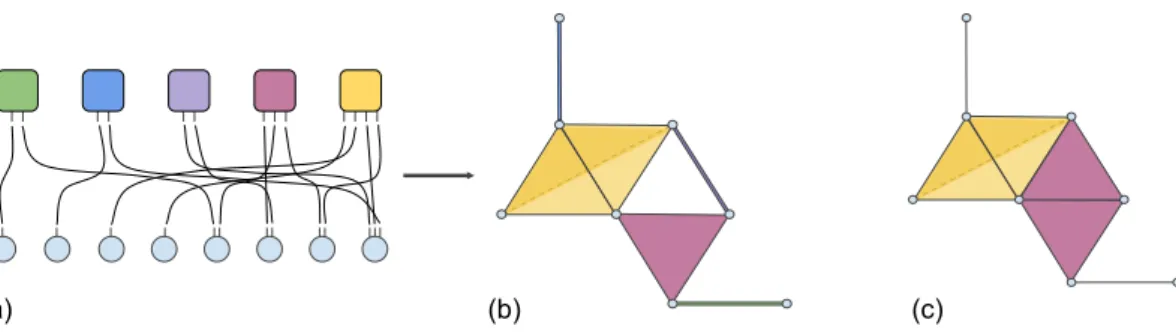
In such a projection, two nodes are considered connected if they are second neighbours in the bipartite graph. This construction simplifies the study of the relationships involved in the data, at the cost of discarding some of the information contained in the original bipartite graph. First, each neighbourhood of a node that is removed during the projection forms a clique in the new graph, but the projection graph does not hold any information on which node it represents. Second, it is not always true that a clique in the projection graph is representing a node that was removed from the original bipartite graph. To retain this information we can associate to every "one-mode" projection a simplicial complex.
(c) (b)
(a)
Fig. 2.1 We can see how projecting the bipartite graph in figure (a), we obtain the simplicial complex in figure (b). This is not a flag complex since the 3-clique[4,5,6] is not a simplex of the complex. In figure (c) we can see the clique complex of the underlying graph.
Theorem 2.1.1. Let G be a bipartite graph with vertex sets {F, V}, GV its
one-mode projections onto the vertex set V. Then it exists a simplicial complex
Σ whose underlying graph is GV.
Proof. Each neighbourhood of a node that is removed during the projection
forms a clique in the new graph, each removed node can be represented as a simplex. The one-mode projection can be seen as substituting one set of
vertices with the simplices that each of them spans, constructing a simplicial complex.
Note that this process does not necessary produce a flag complex since there can be cliques in the one-mode projection whose vertices are not the neighbourhood of a removed vertex, as it is shown in the example in Figure 2.1. Moreover, this process can be inverted, i.e. any simplicial complex can be seen as the one-mode projection of a bipartite graph.
Theorem 2.1.2. For every simplicial complex Σ exists a bipartite graph G
such that one of its two one-mode projections GV is the underlying graph of Σ.
Moreover, the facet size sequence of Σ is equal to the degree sequence of F.
Proof. Consider a graph G with vertex set V ∪F where V is the vertex set of
Σ and cardinality of F is equal to the number of facets in Σ. For each facet
σ ∈ Σ, σ = [v0, . . . , vk], we associate to it a node fσ ∈F, and connect fσ to
the nodesv0, . . . , vk. By construction the projection ofG onto the vertex set
V will give the desired graph.
Courtney-Bianconi model Courtney and Bianconi [28] introduced a
con-figuration model for pure simplicial complexes generalizing the approach on hypergraphs introduced by [45]. Their algorithm generates a pured-simplicial
complex with fixed generalized degree sequence {kr}r≤N, where kr = kd,0(r)
is the number of d-simplices incident on node r, and F = d+11 PN
r=1kr is the
number ofd-simplices or facets of the pure complex (Figure 2.2). The main idea
behind their approach is to introduce a set of F auxiliary nodes representing
Fig. 2.2 A simple example of the construction of a simplicial complex according to the Courtney-Bianconi model. Each auxiliary node has the same number of stubs which are randomly matched with the stubs in the original node set. One can then obtain a regular simplicial complex by projecting the resulting bipartite graph onto the original node set.
Their algorithm then proceeds defining a configuration model for bipartite graphs as follows:
1. kr stubs are placed on each noder = 1, . . . , V, and d+ 1stubs are placed
in each auxiliary nodeµ= 1, . . . , F. At this step each stub is unmatched.
2. a set ofd+1unmatched random stubs of the nodes is chosen with uniform
probability. Without loss of generality we assume that the stubs belong to the set of nodes(r0, . . . , rd).
3. if the nodes(r0, . . . , rd)are all distinct, and no auxiliary nodeµis matched
with the same set of nodes, then with uniform probability an unmatched auxiliary node µ¯ is chosen and matched with the nodes (r0, . . . , rd).
Otherwise the process is re-initialized.
4. if all stubs are matched, then a simplicial complex is constructed projecting the auxiliary nodes onto the original node set.
The rejection procedure step executed at step 3 of the algorithm guarantees that there are no spurious correlations in the structure of the simplicial complex.
In [28] the authors treated in detail the configuration model and the canoni-cal ensemble of simplicial complexes, following the approach used on exponential random simplicial complexes, computing analytically the entropy of the ensem-bles [96]. We refer the reader to [28] for a more detailed study of the statistical mechanics feature of these ensembles.
2.2
Simplicial configuration model
In this section we introduce the simplicial configuration model (SCM) as the maximally random ensemble that generates simplicial complexes with a fixed sequence of maximal clique sizes⃗s={si}i=1,..,F and nodes total degrees
⃗
d={di}i=1,..,N; by a node total degree we mean the number of maximal cliques
that contain that node.
We now show that the random bipartite ensemble of [75] can be re-interpreted as generating simplicial complexes with high probability when
N → ∞. The general idea is to generate a bipartite graph with a vertex set F ∪ V whereF ={f1, ..., fF} represents the set of maximal cliques (or facets)
and whereV ={v1, ..., vN} represents the vertex set of the simplicial complex.
We then assign stubs (half-edges) to each face and vertex according to⃗s and d⃗.
A random matching of the stubs can then be often interpreted as a simplicial complex. That is, it will contain multi-edges with vanishing probability. By multi-edge, we mean that there is two edges or more connecting a node-vertex
vi ∈ V to a node-facefj ∈ F. Moreover it is not always true that the facets size
distribution f⃗. That is, it will contain fully contained neighbourhoods with
vanishing probability, once some amendment to the construction procedure are applied. By fully contained neighbourhoods, we mean that the neighbourhood N(fi)of a node-face fi is completely included in the neighbourhood N(fj) of
node-face fj.
The stub matching scheme can be implemented as follows: 1.a Generate a list of lengthm= PN
i=1di where vi appears di times, for each
i= 1, .., V;
1.b Generate a list of lengthm =PF
i=1si where fi appearssi times, for each
i= 1, .., F;
2 Generate two random permutations, Xv and Xf, of each list;
3 Connect Xv i to X
f
i fori= 1, ..., m;
4 If both the inclusion and multi edges constraints are satisfied, accept the graph, otherwise go back to step 2.
The resulting bipartite graph G(V,F;E) is then interpreted as a simplicial
complex: The neighbours N(fi)of fi are the vertices that form the maximal
simplexfi, for each i, or equivalently, the neighboursN(vi) of vertexvi are the
facets in which nodevi appears.
2.2.1
Correctness of the model
We will now show that with high probability the simplicial complex constructed by our model has facet size distribution⃗s, and total degreed⃗.
We will start proving that with high probability, the simplicial complex will not contain multi-edges following the work by Newman on the configuration model of bipartite graphs [74]. This is a standard calculation that will serve to illustrate the principles that we will apply in the more involved analysis of the next sections.
Theorem 2.2.1. The simplicial complex constructed with the simplicial con-figuration model will not contain multi-edges.
Proof. The probability that there exist an edge(fi, vj) inE is
Pr[(fi, vj)∈E] =
sidj
m , (2.2.1)
since there is a uniform probabilitydj/m of finding vertex vj at any position
in Xv, and there is si occurrences of fi in Xf. More generally, there is a
probability
Pr[(fi, vj)∈E|(fi, vj)ℓ ∈E] =
(si −ℓ)(dj−ℓ)
m−ℓ , ℓ <min{si, dj} (2.2.2)
of having the edge(fi, vj)∈E, provided that is has been already observed ℓ
times. The probability that(fi, vj) appears ℓ times inE is therefore
Pr[(fi, vj)ℓ ∈E] = ℓ−1
Y
λ=0
Pr[(fi, vj)∈E|(fi, vj)λ ∈E] (2.2.3)
For instance forℓ = 2,
Pr[(fi, vj)2 ∈E] =
si(si−1)dj(dj−1)
meaning that the probability that any edge appears two times is Pr[∃ ℓ= 2 ∀(i, j)] = F X i=1 N X j=1 Pr[(fi, vj)2 ∈E] = X i,j si(si−1)dj(dj −1) m(m−1) = = (E[s 2]− E[s])(E[d2]−E[d]) (m−1) . (2.2.5) This goes to zero as 1/m with m → ∞. Since the ensemble is sparse in the infinite limit (fixed average degrees as N → ∞), N must scale linearly inm.
The probability above there goes to zero as1/N with N → ∞. Moreover, since
Pr[(fi, vj)ℓ+1 ∈E]≤Pr[(fi, vj)ℓ ∈E] (from Equation (2.2.3)), then triple (or
quadruple, etc.) edges are even less likely than double edges, and will vanish at least as rapidly as them.
For the constructed simplicial complex to have facet size distribution ⃗s.
This means that the cliques corresponding to the facet-nodes, in the one-mode projection onto the vertex set V, must not be contained into one another. We
show now that with high probability this will not happen.
Lemma 2.2.2. The probability of inclusion between two facets of dimension 2
in a random configuration goes to zero with m → ∞.
Proof. The probability of constructing a k−size simplex σk= [v1, . . . , vk] is
Pr[{fσ, v1), . . . ,(fσ, vk)} ∈E] =
k! Qk
i=1di
From the calculation above we can compute the probability that 2 different facets of size 2 are connected to the same nodes.
Pr[{fa, vi),(fa, vj)} ∈E] = 2 di(dj) m(m−1) (2.2.7) Pr[{fb, vi),(fb, vj)} ∈E|{fa, vi),(fa, vj)} ∈E] = 2 (di−1)(dj−1) (m−2)(m−3) (2.2.8)
The probability that b will be included in a is the following:
Pr[b ⊆a] =X i,j 4 di(di−1)dj(dj −1) m(m−1)(m−2)(m−3) = 4 m(m−1)(m−2)(m−3) 1 2[ X i di(di−1)][ X j dj(dj −1)]− X i d2i(di−1)2 ! = 4 m(m−1)(m−2)(m−3) 1 2(E[d 2]− E[d])2−E[(d2−d)2] (2.2.9) This goes to zero as m−4 with m → ∞. This probability upper bounds the probability of inclusion in a random configuration, which then will also go to zero with m→ ∞.
Theorem 2.2.3. For every σ, τ maximal simplices of size sσ, sτ respectively,
with sσ ≤sτ; we have that
Pr[σ ⊆τ] (2.2.10)
goes to zero as m→ ∞.
2.2.2
Empirical results
Sampling the from SCMThe generalized line-graph representation of simplicial complexes will be the most useful for discussing the sampling algorithm. In this representation, one associates a vertex vi ∈ V to each vertex of the complex, as well as a vertex
fj ∈ F to each of its maximal facets; an edge connectsvi andfj ifvi ∈fj. Each
vi in this line-graph has degree di (the number of facets in which it partakes),
and each vertex representing a facet has degree si (the facet’s size). To each of
these degrees, one may associate labeled stubs, i.e., distinguishable half-edges stemming from the associated node. We have defined the support of the SCM as anysimplicial matching of these labeled stubs, i.e., a matching that yields no multiple memberships of a node to a facet, and no inclusion (a facet containing all the vertices of another facet). For incidence degree and size sequences of finite, a random matching of stubs will often contain at least one inclusion or multiple memberships. An efficient sampler is thus necessary to avoid these culprit. We now show how to sample efficiently from this support with the Metropolis-Hasting algorithm.
Metropolis-Hasting algorithm
The Metropolis-Hasting allows the construction of an ergodic Markov chain over the support of the SCM. One can therefore sample from this chain at regular interval in lieu of sampling constructing random instances of the model from scratch. To ensure ergodicity, a move from a matching X to another
matchingX′ must be accepted with probability a= min ( 1,g(X →X ′) g(X′ →X) P(X′;d, ⃗⃗ s) P(X;d, ⃗⃗ s) ) (2.2.11) where g(X →X′)is the probability of proposing a move from matching X to
matching X′, and P(X;d, ⃗⃗ s)is the likelihood of matching X under the SCM of
degree and size sequences d⃗and ⃗s.
Our proposal distribution is the following: We pick two random edges from the set ofm edges, say, (vi, fj)and (vk, fℓ) and replace them by edges (vi, fℓ)
and (vk, fj). However, if the matching leads to a non-simplicial configuration,
then we give this particular proposal a probability of zero. This means that
g(X →X′) = 1
L(X) , (2.2.12)
where L(X) is the number of “legal” configuration in the neighborhood of
matchingX. Thus, a random move will always be accepted with probability
1, and this move consists of reconnecting two stubs such that the resulting
configuration is simplicial. The resulting chain is, again, ergodic by construction. It is somewhat costly to verify that a matching is simplicial as a whole. One must check that no pair of facet is included, and even clever comparison method will have complexity of the order ofO(f). It is, however, much simpler
to check that a move does indeed lead to a simplicial matching, provided that the base matching is itself simplicial. Indeed, the new matching will only differ in two places, such that one only has to check the facets in which vertices vi
andvj are involved. More specifically, if vertex vi is disconnected from facet fk
of the di facets {f(vi)} of vi will lead to an inclusion of fℓ. If |fℓ| ≥ |f(vi)|,
then an inclusion will occur if
f(vi)−fℓ ={vi}, (2.2.13)
where the minus sign denotes the set difference. If |fℓ| ≤ |f(vi)|, then an inclusion will occur if
fℓ−f(vi) ={vj}. (2.2.14)
A similar condition obviously holds for the facets of vj. Since computing the
set difference is a linear operation, the condition is testable inO(E[d]E[s])time,
which is much more efficient, especially in sparse complexes.
The data sets
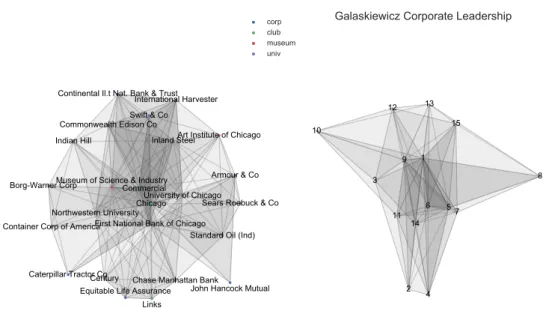
We applied the simplicial configuration model to the randomization of two data sets depicting the corporate leaderships in Chicago [5], and in Minneapolis-St.Paul [44].
The first example data set we consider is the affiliation data set of corporate directors from 1962 in the Chicago area studied by Barnes and Burkett [5]. This data set contains the affiliation between 24 companies and 20 people in a leadership position in those companies. To construct the simplicial complex we considered as vertices the companies and each facet represents a person in a leadership position in the companies represented by the vertices.
As another example, we considered the affiliation data set of club and board memberships of corporate executive officers studied by Galaskiewicz [44] as part of his research on the urban grants economy in Minneapolis-St.Paul. We followed the approach adopted by Faust [39] and focused on a subset of 26 CEOs and 15 clubs/boards from Galaskiewicz’s data. We then constructed a second simplicial complex in as done for the Barnes-Burkett data set. The simplicial complexes from these data sets are represented in figure 2.3.
Chicago
John Hancock Mutual Container Corp of America
Art Institute of Chicago Inland Steel
Northwestern University Commercial
Sears Roebuck & Co International Harvester
Museum of Science & Industry
Chase Manhattan Bank Equitable Life Assurance
University of Chicago Continental Il.t Nat. Bank & Trust
Armour & Co Caterpillar Tractor Co Links Century Borg-Warner Corp Indian Hill Swift & Co
First National Bank of Chicago Standard Oil (Ind) Commonwealth Edison Co
corp club museum univ
Barnes-Burkett Corporate Leadership
1 2 3 4 5 6 7 8 9 10 11 12 13 14 15
Galaskiewicz Corporate Leadership
Fig. 2.3 Visualization of the simplicial complex generated from the Barnes-Burkett data set (left), and the Galaskiewicz data set (right). Each simplex (in gray) represents a person in a leadership position in the companies represented by the vertices of the complex.
To further study the structure of the simplicial complexes we constructed from data, we computed its homological cycles. We will introduce in detail the concept of homology in the next chapter (sec. 3.3). We will give now a practical idea of the concept.
Homology of dimensionk is a functor that assigns to each simplicial complex
a vector spaceHk. The generating elements of the vector space Hk are called
the homological k-cycles. In low dimensions the homological cycles can be
interpreted easily as particular features of the simplicial complex: the 0-cycles represent the connected components, the 1-cycles are cordless cycles not closed by triangles, the 2-cycles are voids closed by a triangle tessellation. These structure can be meaningful in understanding particular features of a data set. These assumptions can then be validated comparing it with the empirical probability distribution of the ensemble generated by our model.
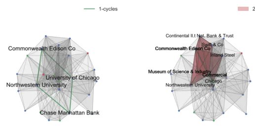
For each constructed simplicial complex we computed its homological cycles (javaPlex library [91]). In Figure 2.4 we show the1 and2 dimensional cycles
of the simplicial complex constructed from the Barnes-Burkett data sets. The
1-dimensional cycle can be interpreted a set of institutions or corporations for
which corporate interlock is not as tightly bound as in the rest of the data set. the only two universities in the data set are present in this cycle. Furthermore, we detected three2-dimensional cycles in the simplicial complexes. These voids
can be interpreted as a set of institutions or corporations for which there is no single person in a leadership position in all of them. It is interesting to notice that these voids are connected to each other through and edge or a triangular face, as shown in figure 2.4.
To validate these results we sampled the ensemble generated by the simplicial configuration model with facet size and incidence degree sequences fixed by the Barnes-Burkett, and the Galaskiewicz data sets. We sampled the two ensembles with the algorithm described above, and computed the homology of each sampled simplicial complex.
Commonwealth Edison Co
Chase Manhattan Bank Northwestern UniversityUniversity of Chicago
1-cycles
Barnes-Burkett Corporate Leadership
Commonwealth Edison CoSwift & Co
Museum of Science & Industry Commercial Continental Il.t Nat. Bank & Trust Commonwealth Edison Co
Commercial Museum of Science & Industry
Northwestern University Commonwealth Edison Co Inland Steel Commercial Chicago 2-cycles
Barnes-Burkett Corporate Leadership
Fig. 2.4 Visualization of the 1-dimensional cycle (in green) and of the 2-dimensional cycles (in red) of the simplicial complex generated from the Barnes-Burkett Corporate Leadership data set.
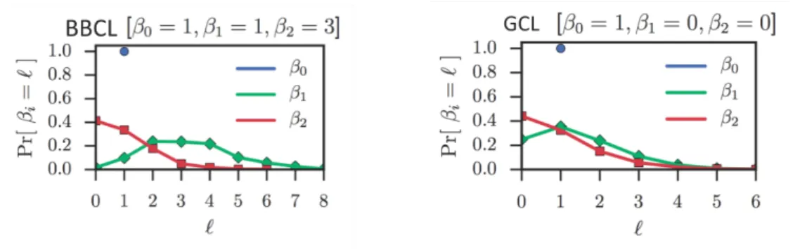
In figure 2.5 we show the sampling distribution of the number of cycles in a simplicial complex, called Betti number, for the two ensembles. We can see that in both cases the probability to generate a simplicial complex with only one connected component is 1, which might depend on the small sizes
of the data sets we considered. Moreover, we can notice how unlikely is the emergence of 1 and 2- dimensional cycles in the configuration generated from
the Barne-Burkett data set, validating our findings. On the other hand, from the sampling distribution obtained on the Garlaskewicz data’s ensemble we can deduce that the absence of homology in the real simplicial complex is quite probable. Meaning that, in this case, homology might not be the best tool to analyse the data.
Fig. 2.5 Sampling distribution for the Betti number (dimensions 0,1, and2) of two different ensembles of simplicial complexes generated with the simplicial configuration model. On the left, the ensemble with fixed size distribution and incidence degree distribution from the Barnes-Burkett Corporate Leadership data set, whose real Betti numbers are β0 = 1, β1 = 1, β2 = 3. On the right, the ensemble with fixed size distribution and incidence degree distribution from the Galaskiewicz data set, whose real Betti numbers are β0= 1, β1 = 0, β2 = 0.
2.3
Generating random simplicial complexes
The simplicial configuration model can be used to generat