approximation techniques and a
continuous-time resource selection
method
Yi-Shan Wang
A thesis submitted in partial fulfilment of the requirements for the degree of Doctor of Philosophy
The University of Sheffield
Faculty of Science
School of Mathematics and Statistics
Firstly, I would like to express my gratitude to my supervisor, Dr Potts, for the continuous support of my PhD study, for his guidance and patience. His detailed comments on my writing helped me transform my obscure sentences into understandable paragraphs.
Besides my supervisor, I would like to thank Prof Blackwell for his support on statistical inference, and thank Dr Merkle for providing the mule deer data. I also would like to thank Ministry of Education of Taiwan for financial support. My sincere thanks also goes to friends from Christ Church Fulwood in Sheffield. They constantly asked me about my progress and prayed for me.
Finally, I would like to thank my family: my husband, Caleb, our kids, my mum and my brother for their love and support.
This thesis consists of two parts. First, I investigate the effect of using three partial differential equation (PDE) techniques on analysing some simple animal movement models. Results of examining a biased random walk show that an old approach from Patlak’s work in 1953 can give a very poor approximation even in this very simple case, while more recent methods correctly describe the movement process. By analysing central-place foraging models and movement in heterogeneous landscapes, I show that more recent PDE techniques can provide more accurate approximations of space use patterns when the kernel describing the movement is sufficiently smooth. However, for non-smooth movement kernels, all methods can result in quantitatively misleading approximations. This analysis provides an insight into the conditions under which the PDE methods might perform better.
Second, I present two continuous-time modelling frameworks for analysing animal movement depending on selection of resources over the whole landscape or in the surrounding area. The models are parameterised by a Markov chain Monte Carlo (MCMC) algorithm, allowing for movement decisions made at any time. Based on these frameworks, I generate simulations in various situations, including mi-gration and foraging in patchy or rasterised landscapes. Analysis of simulated trajectories reveals that the inference algorithm can successfully capture the pa-rameter values used in simulations in most cases. I also fit the migration model to spring migration data of some mule deer (Odocoileus hemionus). The re-sults imply that migration might be explained by the trade-off between resources and travel distance. This work addresses some limitations of methods relying on discrete-time movement models and therefore provides an advanced tool for understanding movement driven by environmental factors.
1 Introduction 1
1.1 A comparison of approximation techniques . . . 3
1.2 A continuous-time resource selection method . . . 6
1.2.1 Previous approaches . . . 10
1.3 Thesis outline . . . 13
2 Partial differential equation techniques for analysing animal move-ment 15 2.1 Movement kernel analysis . . . 16
2.1.1 Hyperbolic Scaling method . . . 17
2.1.2 Moment Closure method . . . 18
2.1.3 Patlaks approach . . . 19
2.2 Comparison between the PDE techniques . . . 20
2.2.1 Evaluation of short-term estimation . . . 21
2.2.2 Evaluation of long-term estimation . . . 22
2.3 An analytic example: a biased random walk . . . 23
2.4 A central-place foraging model with discontinuous mean velocity . 26 2.4.1 Analysis of movement kernel k1 τ(z|x) by the PDE techniques 27 2.4.2 Numerical analysis of movement kernel k1 τ(z|x) . . . 29
2.5 A central-place foraging model with continuous mean velocity . . 31
2.5.1 Analysis of movement kernel k2 τ(z|x) by the PDE techniques 32 2.5.2 Numerical analysis of movement kernel kτ2(z|x) . . . 35
2.6 A central-place foraging model with differentiable mean velocity . 35 2.6.1 Analysis of movement kernel k3 τ(z|x) by the PDE techniques 38 2.6.2 Numerical analysis of movement kernel k3 τ(z|x) . . . 40
2.7 Movements on heterogeneous landscapes . . . 42
2.8 Summary . . . 50
3 Resource selection analysis by continuous-time movement mod-els 51 3.1 Modelling framework . . . 52
3.2 Inference by Markov chain Monte Carlo . . . 54
3.3 Migration models . . . 58
3.3.1 Simulations . . . 59
3.3.2 Inference from simulations . . . 61
3.4 Resource depletion-renewal models in a patchy landscape . . . 69
3.4.1 Simulations . . . 69
3.4.2 Inference from simulations . . . 71
3.5 Resource depletion-renewal models in a raster landscape . . . 75
3.5.1 Simulations . . . 75
3.5.2 Inference from simulations . . . 76
3.6 Discussion . . . 83
4 Analysis of movements following a resource gradient 86 4.1 Modelling framework . . . 86
4.2 Inference by Markov chain Monte Carlo . . . 89
4.3 Simulations . . . 90
4.4 Inference from simulated data . . . 91
4.5 Discussion . . . 98
5 A case study of mule deer data in the Greater Yellowstone Ecosys-tem 100 5.1 The data and models . . . 101
5.1.1 The movement and resource data . . . 101
5.1.2 Three models for resource selection . . . 101
5.2 Inference from data . . . 102
5.3 Discussion . . . 107
6 Discussion and Conclusions 110 6.1 Comparison of three PDE approximation methods . . . 111
6.2 The modelling framework for analysing movement responses to resources . . . 114
6.2.1 Comparisons with previous work . . . 115
6.2.2 Possible future directions . . . 116
6.3 Summary . . . 118
A Measuring distance between distributions by Euclidean distance121 B A comparison between continuous-time discrete-space models
3.1 The overall performance of the inference method method when analysing simulations in Chapter 3 . . . 78
5.1 The comparison of models for the mule deer data, where all 3 models can be fitted . . . 105 5.2 The comparison of models for the mule deer data, where all 3
models can be fitted . . . 106 5.3 The comparison of models for the mule deer data, where 1 or 2
models can be fitted . . . 107
1.1 Mean velocity functions of central-place foraging models . . . 5
1.2 Examples of heterogeneous resources . . . 5
1.3 A landscape with five food patches to choose from . . . 7
1.4 A simulated trajectory in a patchy landscape . . . 8
1.5 A simulation of movement following a local resource gradient . . . 9
1.6 Migration data of a mule deer and relevant resource data . . . 11
2.1 An analytical example of using the PDE methods . . . 26
2.2 An example of a discontinuous mean velocity function . . . 27
2.3 Discontinuous mean velocity movement model . . . 30
2.4 An example of a continuous mean velocity function . . . 33
2.5 Continuous mean velocity movement model . . . 36
2.6 Continuous mean velocity movement model . . . 37
2.7 An example of a differentiable mean velocity function . . . 38
2.8 Differentiable mean velocity movement model . . . 41
2.9 Differentiable mean velocity movement model . . . 42
2.10 More examples of using the PDE methods . . . 48
2.11 Movements in a landscape with smooth resource change . . . 49 viii
3.1 Augmentation of a subset of observed data . . . 56 3.2 A simulation of migration . . . 60 3.3 Trace plots of MCMC chains . . . 61 3.4 Posterior distributions derived when analysing a simulation of
mi-gration . . . 62 3.5 The relationship between iterations before converging and
param-eters in simulations of migration . . . 63 3.6 The log ratios between sample means and real values when
apply-ing MCMC inference on simulations of migration . . . 65 3.7 The relationship between the efficiency of the MCMC algorithm
and κ . . . 66 3.8 The relationship between the accuracy of the MCMC algorithm
and κ . . . 67 3.9 The number of iterations before converging when using different
initial values in MCMC inference on a simulation of migration . . 68 3.10 A simulated trajectory in a patchy landscape with the resource
depletion-renewal model . . . 70 3.11 Posterior distributions derived when analysing a simulation of
move-ment in a patchy landscape with the resource depletion-renewal model . . . 71 3.12 The relationship between iterations before converging and
param-eters in simulations of movements depending on resource depletion or renewal in a patchy landscape . . . 72 3.13 The log ratios between sample means and real values when
apply-ing MCMC inference on simulations of movements dependapply-ing on resource depletion or renewal in a patchy landscape . . . 73 3.14 The number of iterations before converging when using different
initial values in MCMC inference on a simulation of movements dependent on resource depletion or renewal in a patchy landscape 74
3.15 A simulated trajectory in a raster landscape with the resource depletion-renewal model . . . 75 3.16 Posterior distributions derived when analysing a simulation of
move-ment in a raster landscape with the resource depletion-renewal model 76 3.17 The relationship between iterations before converging and
param-eters in simulations of movements depending on resource depletion or renewal in a raster landscape . . . 77 3.18 The log ratios between sample means and real values when
apply-ing MCMC inference on simulations of resource depletion-renewal models in a raster landscape using different b . . . 79 3.19 The log ratios between sample means and real values of when
applying MCMC inference on simulations of resource depletion-renewal models in a raster landscape using different v . . . 80 3.20 The log ratios between sample means and real values when
apply-ing MCMC inference on simulations of resource depletion-renewal models in a raster landscape using different β . . . 81 3.21 The number of iterations before converging when using different
initial values in MCMC inference on a simulation of movements dependent on resource depletion or renewal in a raster landscape . 82
4.1 Neighbouring patches used to determine resource gradient in a rasterised landscape . . . 88 4.2 a simulation of movement following a resource gradient . . . 90 4.3 Posterior distributions derived when analysing a simulation of
move-ment following a resource gradient . . . 92 4.4 The relationship between the efficiency of the MCMC algorithm
and κ for the gradient-following movement model . . . 92 4.5 The relationship between the accuracy of the MCMC algorithm
4.6 The number of iterations before converging when using different initial values in MCMC inference on a simulation of movements following local resource gradient . . . 94 4.7 The relationship between iterations before converging and
param-eters in simulations of movements following local resource gradient 95 4.8 The log ratios between sample means and real values when
apply-ing MCMC inference on simulations of gradient-followapply-ing move-ments using different values for the drift coefficient . . . 96 4.9 The log ratios between sample means and real values when
apply-ing MCMC inference on simulations of gradient-followapply-ing move-ments using different values for the diffusion coefficient . . . 97
5.1 A case study of mule deer data . . . 102 5.2 Inference from mule deer data using NDVI and integrated NDVI . 103 5.3 Inference from mule deer data using IRG . . . 104 5.4 A simulated trajectory of mule deer migration . . . 104 5.5 Distance between winter range centres and days between departure
dates . . . 109
A.1 Discontinuous mean velocity movement model (Euclidean distance) 122 A.2 Continuous mean velocity movement model (Euclidean distance) . 123 A.3 Continuous mean velocity movement model (Euclidean distance) . 124 A.4 Differentiable mean velocity movement model (Euclidean distance) 124
B.1 Simulated trajectories of movement following a local resource gra-dient . . . 128 B.2 The density of estimated α obtained using R package ctmcmove . 129 B.3 The posterior distributions derived from analysing the simulated
Introduction
Animal movement plays a central role in understanding relationships and patterns in ecosystems. For instance, population distribution or space use patterns can be regarded as the consequence of movements (B¨orger et al., 2008). Movements can also stem from conspecific and interspecific interactions as well as interactions between animals and the environments (Lewis and Murray, 1993; Chetkiewicz and Boyce, 2009; Vanak et al., 2013).
By analysing animal movements, researchers have attempted to derive spatial pat-terns, including the formation of home ranges and territories (Moorcroft et al., 1999; B¨orger et al., 2008; Bateman et al., 2015; Potts and Lewis, 2016b; Merkle et al., 2017), utilisation distributions (Benhamou, 2011; Signer et al., 2017; Wil-son et al., 2018), the space use patterns resulting from competition (Potts and Petrovskii, 2017) and the influence of spatial attributes (Forester et al., 2009). Furthermore, studies of movement are also key to our insight into other aspects of the living world because movement governs not only the life of individuals but also patterns at scales from population, community to ecosystem (Nathan et al., 2008). In addition, the advance in tracking technology has enabled the collection of high-resolution data, which considerably improves our knowledge of the underlying mechanisms, causes and consequences of movement (Kays et al., 2015).
Behind the great importance of the analysis of movement in understanding the 1
living world, some challenges make it difficult to analyse movement data. Some major problems arise from behavioural changes, autocorrelation between obser-vations and observation errors in data (Gurarie et al., 2009). The change of movement behaviour can stem from the heterogeneity of the environment and different activities in life and may have a greater impact on scaling up individual movement to space patterns than environmental factors do (Morales and Ellner, 2002). Much research has been devoted to the identification of behavioural modes in order to capture the scenario of animals’ life such as migration more precisely (Gurarie et al., 2009; Bunnefeld et al., 2011; Pedersen et al., 2011; Fleming et al., 2014a; Bastille-Rousseau et al., 2016). The autocorrelation in position and ve-locity comes from the fine scale of data collection and can be incorporated in movement models such as a discrete-time correlated random walk (CRW) and a continuous-time stochastic movement model (e.g. the Ornstein-Uhlenbeck pro-cess). Beyond the consideration of autocorrelation in a movement model, Fleming et al. (2014b) and Fleming et al. (2017) developed methods to facilitate the use of continuous-time models to efficiently deal with autocorrelated data. For tackling the complexity caused by observation errors, a promising tool is a state-space model (Patterson et al., 2008; Albertsen et al., 2015), which uses a model to explicitly incorporates observation errors in addition to a model for movement process. Although this thesis will not focus on resolving these issues, they could be taken into account in future research based on the work of this thesis.
This thesis is composed of two topics related to the derivation of spatial patterns from animal movements. The first is to compare the accuracy of approximation methods for predicting population space use patterns from individual movement rules. The second introduces two modelling frameworks and an algorithm for inference to infer the preferences of animals for resources from movement data in two separate situations. In one case, an animal is assumed to assess the resources across the landscape when making movement decisions, similar to Ford (1983) and Mitchell and Powell (2004), whereas the other modelling method considers only the resources in the immediate vicinity of the animal’s location, similar to Preisler et al. (2013). Real situations may reside in between these two extremes.
§1.1 A comparison of approximation techniques
The first topic discussed in this thesis focuses on methods for analysing individual movement mechanisms, represented by a function termed amovement kernel. In this part of the thesis, I will only consider models in a 1-dimensional space and not involving direction. A movement kernel kτ(z|x) describes the probability of
an animal moving to a place z in a (typically small) period of time τ, given its current location x. This probability can be affected by factors such as distance to the destination from the animal’s position, environmental conditions and in-teractions between animals and these factors can be integrated into an extended movement kernel (Potts, Mokross and Lewis, 2014). Thus it is convenient to use a movement kernel to describe individual movement rules, as the studies in Rhodes et al. (2005), where movements depend on the location of the animal’s home range.
However, a movement kernel only represents the probability of selecting a position in a relatively short period of time compared to an animal’s lifetime. On the other hand, understanding an ecosystem often involves long-term patterns at population level, described by some key information such as the distribution and abundance of a species. Therefore, techniques are necessary to scale up the decision-making process at individual level, described by a movement kernel, to space use patterns at population level. To scale up individual movement to long-term patterns, it is conceptually straightforward to use the Master Equation (ME), which propagates the movement kernel forward in time and is commonly used (Moorcroft and Barnett, 2008; Potts, Bastille-Rousseau, Murray, Schaefer and Lewis, 2014; Merkle et al., 2018):
u(x, t+τ) = Z ∞
−∞
kτ(x|y)u(y, t)dy, (1.1)
where the function u(x, t) is the probability density of the animal’s position x at time t. In practice, it requires the iteration of Equation (1.1) until the difference between distributionsu(x, t) andu(x, t+τ) is sufficiently small to obtain the long-term distribution at steady state. However, calculating this integral repeatedly can be computationally demanding, so more efficient approximation methods are
favoured.
Some techniques have been developed to approximate the long-term distribution by converting the ME to a partial differential equation (PDE) (e.g. Codling et al. (2008), Section 2.2). Using the solution to a PDE at steady state to estimate the long-term distribution is much more efficient than iterating the ME. Nevertheless, these approximation techniques usually require particular assumptions such as omitting higher order moments in the system to make it tractable. The extent to which these approximations are reliable is unknown. For instance, a second-order moment closure assumes that moments at orders higher than two can be expressed by only the first and second moments. However, such a closure can make a poor approximation of spatially structured populations if the spatial features involve much information at higher orders (Murrell et al., 2004). Therefore, my first object was to investigate the accuracy of the approximations using three such techniques, all of which are formulated in PDEs, and draw a comparison between them. This investigation was performed by examining either long-term or steady-state distributions in various example cases, described in detail below.
The oldest method was developed in the mid-20th century by Patlak (1953) and popularised in the context of animal movement by Turchin (1991). Hillen and Painter (2013) reviewed two more recently developed methods, namely the Hyper-bolic Scaling and Moment Closure methods. Potts et al. (2016) used these three methods to examine animal distributions near a habitat edge in a one-dimensional interval composed of two segments featuring different spatial attributes. In this thesis, I consider the application of these PDE methods on the whole 1D real line as well as a finite interval in several situations.
First, I compared the three approximate methods by using them to examine a biased random walk, biased towards a fixed direction and simple enough that the PDEs involved can be solved analytically. This shows Patlak’s method gives a poor approximation, while the other methods provide an exactly correct pre-diction. Since Patlak’s approach can fail even a very simple example, it may also produce misleading results when analysing a more complicated movement. Therefore, it needs further consideration to understand the effect of the three methods on the steady-state distribution when examining more general cases.
(a) (b) (c)
Figure 1.1: Mean velocity functions of central-place foraging models with different levels of con-tinuity. (a) A discontinuous mean velocity function. (b) A continuous mean velocity function, having non-differentiable points (c) A differentiable mean velocity function.
Subsequently, I investigated cases where the PDEs derived could be solved an-alytically at steady state to obtain the long-term distributions. Such examples considered include three types of central-place foraging movement models. With the central place being located at the origin, the mean velocity functions of these models have different levels of continuity: the first type has a discontinuous point at the central place (e.g. Figure 1.1a), the second is continuous over the real line but has two non-differentiable points near the central place (e.g. Figure 1.1b) and the last is differentiable everywhere (e.g. Figure 1.1c). These three central-place foraging models were examined to reveal how changes in velocity affect the results of using the approximate methods.
(a) (b)
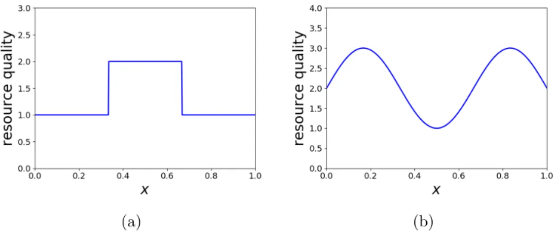
Figure 1.2: Examples of heterogeneous resources. (a) Resource quality with discontinuous jumps. (b) Resource quality which changes smoothly.
heterogeneous resources of two types, one of which has discontinuous jumps (e.g. Figure 1.2a) and the other changes smoothly (e.g. Figure 1.2b). These two types of resources were considered to understand the impact of changes in resources on the approximation of long-term distribution. This is similar to the strategy which examines central-place foraging models with different level of smoothness. In general, the results of examining these cases indicate that the PDE methods can provide poor approximations if the movement kernel is non-smooth and better estimates if the movement kernel is sufficiently smooth.
§1.2 A continuous-time resource selection method
The second part of the thesis introduces tools for analysing animals’ movement responses to resources changing over time. As animals use resources in space selectively, understanding how they make selection decisions is central to gaining insight into underlying movement mechanisms (Cagnacci et al., 2010). A widely used tool for representing the selection of resources is the resource selection anal-ysis (RSA), often relying on a resource selection function (RSF) (Manly et al., 2002), which takes values proportional to the probability of using a resource unit. When applying an RSF, a used resource unit is often compared to some other resource units which are available but not used. However, it may not be straight-forward to define the availability of a resource unit and may not be realistic to assume that every unit across the land is equally available.
This problem of defining the availability of a resource unit has been resolved by step selection analysis (SSA) (Fortin et al., 2005; Forester et al., 2009; Thurfjell et al., 2014). Instead of considering the selection of locations in space, SSA examines the selection of ‘steps’, defined by linking two consecutive observed points. Each used step is compared to some random steps starting from the same beginning position of the used step. In this way, the availability of a step is naturally constrained by the animal’s mobility, which can be described by the probability of moving from the starting to end points of the step. Furthermore, SSA has been extended to allow simultaneous estimation of the parameters of resource selection and movement, since movement traits such as velocity may be
influenced by resource selection. This extension of SSA is termed integrated step selection analysis (iSSA) (Avgar et al., 2016).
Although SSA and iSSA have successfully enhanced the analysis of resource selec-tion by considering mobility, there are some drawbacks of SSA and iSSA because they rely on a time movement modelling framework. Since a discrete-time movement model requires data to be collected with fixed discrete-time intervals, this makes it difficult to manage data irregular in time (McClintock et al., 2014). Moreover, SSA and iSSA are based on the assumption that the animal decides to move exactly at points observed and never changes its mind between two ob-servations. As a result, when applying SSA or iSSA, the time scale needs to correspond to decisions to move to reach a correct conclusion (Thurfjell et al., 2014). Only a few types of discrete-time movement models are robust enough to be adjusted to match the temporal scale to movement processes (Schl¨agel and Lewis, 2016).
Figure 1.3: A landscape with five food patches to choose from. The blue star is the animal’s location and circles A1 to A5 are food patches. The animal is assumed to choose its target
patch by comparing the attractiveness of patches and selecting the most attractive patch.
To take advantage of incorporating movements into RSA yet circumvent the prob-lems of using a discrete-time model, I embed a resource weighting function, which reflects the preferences of the animal, into a continuous-time movement model. For example, in Figure 1.3, there are five food patches in the landscape and I as-sume the animal decides which patch to move towards by comparing the patches’ attractiveness, which is evaluated by a resource weighting function. After deter-mining the destination, a continuous-time movement model is fitted to describe
(a) (b)
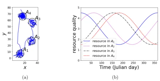
Figure 1.4: A simulated trajectory in a patchy landscape. (a) A simulation of migration gener-ated on the assumption that the animal moves in response to the change of resource qualities in food patches. The animal was attracted to patchA1 in the beginning and subsequently moved
to patches A2, A3 and A4. At last, it travelled back to patch A1 (b) Resource qualities in the
patches in Figure 1.4a.
how the animal approaches its target place. A simulated trajectory generated on these assumptions is shown in Figure 1.4a along with the resource qualities in food patches, given in Figure 1.4b. This scenario forms the basis of my first modelling framework, where the animal moves relying on complete knowledge of its envi-ronment. This strategy is the first to be able to consider movements triggered by factors in remote areas rather than being limited to decision-making at the scale of observation, although the idea of taking places far away into consideration has been mentioned in Bastille-Rousseau et al. (2018).
The second modelling framework assumes that animals move in response to lo-cal clues instead of considering resources across the land. This represents the situation where the dependence on perception predominates over the reliance on memory (cf. Bracis and Mueller (2017)). In this case, an animal is assumed to move in the direction up local resource gradient, which is calculated by evaluating the resource quality of nearby areas using a resource weighting function. Figure 1.5 gives an example. This is similar to movements with a drift term described by a potential function (Brillinger, 2010) and my modelling framework also allows for redirection by reassessing local resource qualities at any time.
Figure 1.5: A simulation of movement following a local resource gradient. The patch colours, yellow, light green and dark green, represent low, medium and high resource qualities, assumed to be fixed in this example. The star is one of the simulated locations and the arrow points the direction up the resource gradient, determined by the resource qualities in patches AN, AS,
AE and AW, where N, S, E, W stand for north, south, east and west. The animal is assumed
to move in the direction up the resource gradient with some uncertainty.
into account the reality that movement decisions can be made at any time by aug-menting the data with points where decision-making might occur, similar to the imputation of paths in Hanks et al. (2015). Moreover, my method is an advance in RSA as it is able to consider resource selection beyond the observation scale. The inference algorithm has been applied on both simulated and real data and the results show that the inference method is reliable at simultaneously param-eterising a resource selection function and a movement process from movement data in a wide range of scenarios.
The simulated data examined consists of examples generated from the two mod-elling frameworks, one of which compares resource units across the landscape and the other only assesses local resources. For the former framework, three dif-ferent situations were considered. In the first situation, I simulated movement in a landscape with several food patches. The resource qualities in the patches were assumed to change seasonally and be independent of the foraging activities of animals. This was used to simulate the scenario of migration and Figure 1.4 shows such an example. The second situation also used patchy landscapes but assumed the opposite for resource qualities. In this case, the resource qualities were depleted or renewed dependent on the time the animal spends in a resource patch. This can resemble movements of an animal in its home range. The third
situation was a raster-landscape version of the second. That is, simulated tra-jectories were generated in a rasterised landscape on the assumption that the resource in a cell was consumed as a result of the animal’s presence in that cell and grew otherwise. Here, every food patch in a patchy landscape and every cell in a raster landscape is a resource unit, whose quality is assessed when deciding the target place of movement.
Simulated trajectories generated from the other modelling framework were in raster landscapes and the decision on movement direction only involved the four neighbouring cells in the north, south, east and west of the animal’s current position (Figure 1.5). These simulated trajectories model movement relying on the perception of local clues, in contrast to the first modelling framework, which assumes a movement decision is made by assessing every resource unit, both far and near, in the landscape.
I applied the first modelling framework to analyse the spring migration data of 28 mule deer (Odocoileus hemionus) in the Greater Yellowstone Ecosystem to demonstrate the methodology and give a possible explanation for factors driving migration. The time and location data of individuals were collected every 2 hours from March to August 2016. The data points in the winter and summer ranges formed distinguishable clusters as the distance travelled from winter to summer ranges was about 75 kilometres on average. For some individuals, there were also small clusters of data points along the migration path. To represent resource qualities, I used the normalised difference vegetation index (NDVI) and instantaneous rate of green-up (IRG) over the area where the mule deer were observed. In addition, I also considered resource qualities defined by the integral of NDVI from a time of observation to the end of summer. Figure 1.6 shows the migration data of a mule deer along with resource qualities in recognised foraging patches.
1.2.1 Previous approaches
The goal of the second part of the thesis is to develop a tool for RSA by integrat-ing a RSF into a continuous-time movement model rather than a discrete-time
(a)
(b)
(c) (d)
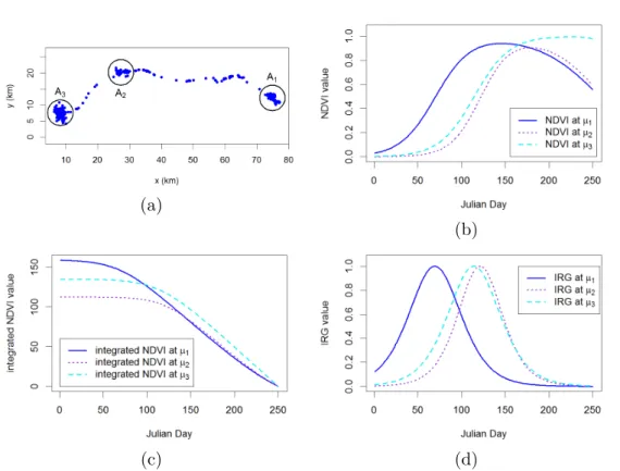
Figure 1.6: Migration data of a mule deer and relevant resource data. (a) The location data collected from March to August 2016 in the Greater Yellowstone Ecosystem. The circles A1,
A2 and A3 are identified patches with centres µ1, µ2 and µ3 respectively. The deer migrated
from patch A1 to patch A3 via patch A2. Resource data were daily values from Julian day 1
to day 250 in 2016: (b) NDVI values at patch centres; (c) integrated NDVI at patch centres; (d) IRG values at patch centres.
movement model. In this review, I will focus on the modelling framework for considering resource selection across the whole space since this framework is the major achievement of the thesis. Here, I give a short review of a commonly used continuous-time movement model, the Ornstein-Uhlenbeck (OU) process, to ex-plain why this is an ideal choice for my modelling framework. In addition, I briefly introduce some previous work on continuous-time movement models and how they relate to RSA to show gaps my work intends to close.
An OU process describes a biased random walk towards a centre of attraction and has been used for studying animal movement for a while. For instance, Dunn and Gipson (1977) studied the estimation of home range by using an OU pro-cess to represent movements attracted to a central place. Building on the idea
of Dunn and Gipson (1977), where individual movement is described by only a single OU process, Blackwell (1997) generalised the OU model by using differ-ent OU process for differdiffer-ent situations. These differdiffer-ent situations may stand for different locations of interest or different behavioural states such as resting and feeding. With a mixture of movement processes and assuming animals switch between these processes while moving, Blackwell (1997) has used such a model, termed a switching OU model, to describe more general space use patterns such as (i) movement with two centres of attraction, (ii) movement with large-scale excursions and (iii) movement with different behavioural states. These exam-ples provide an initial step to model movement decisions made according to the selection of resources, which can be nearby or far away.
Parameterisation of the models is achieved by Bayesian inference strategies (Black-well, 2003) and subsequent studies have extended the OU modelling framework to include heterogeneous spatial conditions (Harris and Blackwell, 2013; Blackwell et al., 2016). Since the OU models are ready to incorporate both heterogeneous landscapes and different behavioural states, it has great potential to strengthen the analysis of resource selection by inserting a RSF into an OU model. This was a direction for further research suggested by Schick et al. (2008) that the incor-poration of a RSF in a movement model would provide a better understanding of the link between the environment, behavioural states and movement decisions. In particular, when using a switching OU model, a RSF can be used to identify the place where the animal intends to approach and thus can determine which OU process to follow at a specific moment. The incorporation of RSA into the OU framework in this way is the primary purpose of the second part of this thesis. The use of an OU process in RSA has been proposed by Johnson et al. (2008). In Johnson et al. (2008), an OU process describes the probability of moving from one fix to the next to represent the density of available resources. However, they did not include possible decision changes between observations.
Apart from the switching OU model, there are several studies devoted to incor-porating resource selection into a continuous-time movement model. An example is Horne et al. (2007), which introduced the Brownian bridge movement model (BBMM), which links pairs of two successive observations to estimate movement
paths. Estimation of movement paths can bring about the identification of places which are frequently used and then these areas can be related to environmental conditions to understand the selection of resources (Horne et al., 2007). However, as a Brownian bridge connecting two observations assumes a higher frequency of use in the extending area over the straight line between the two locations, that is, a step in SSA, it may also lead to misinterpretation of resource selection as SSA may do. For example, for cases other than crossing a road as in Horne et al. (2007), this approach may miss the situation where the animal aims at an area in the distance and have to pass a certain place which is in fact not of great interest. In addition, Horne et al. (2007) did not consider changes of movement decision along the path.
Hanks et al. (2015) proposed a model where the movement path is discretised and a resource selection function is embedded in the transition rate between neighbouring cells. However, it only focuses on transitions within a local area and implicitly assumes that the decision-making process is coincident with the scale of observation. It does not consider the situation where movement might be motivated by a long-term goal such as the migration between seasonal ranges. Therefore, there is a lack of a model for simultaneously representing movement depending on resource selection at large scales in continuous time and considering decisions made between observations. On the other hand, the combination of a switching OU model and a RSF in this thesis provides a useful tool in this regard.
§1.3 Thesis outline
In Chapter 2, I investigate the accuracy of three partial differential equation (PDE) methods for estimating location redistributions by comparing approxima-tions with actual distribuapproxima-tions arising from movement kernels. I demonstrate the performance of the PDE methods on different assumptions for movement strate-gies and in different spatial conditions. Most of the contents in this chapter has been published in Wang and Potts (2017).
To understand how animals move in response to environmental conditions, Chap-ter 3 introduces a modelling framework for resource selection analysis using
continuous-time movement models. I use a resource selection function to identify the attraction centre of movement in space and a switching Ornstein-Uhlenbeck (OU) process to describe movements drifting to the most attractive place in the landscape.
Chapter 4 uses similar strategies as Chapter 3 but describes movements in a dif-ferent situation, where only local information is considered. I describe movements using a random walk in the direction up the local resource gradient, which is de-termined by comparing the value of the resource selection function in the vicinity of the animal’s position.
The movement modelling framework in Chapter 3 is applied to mule deer (Odocoileus hemionus) data in Chapter 5. I fit a migration model built on the framework in Chapter 3 to the migration data, using Bayesian inference techniques.
Partial differential equation
techniques for analysing animal
movement
Most contents of this chapter has been published in Wang and Potts (2017). Animal movement contributes to population distributions and the formation of space use patterns. By assuming all individuals move according to the same rule, the probability of an individual being at a certain position at a given time can represent the population density (Turchin, 1991). A movement rule can be represented by a movement kernel, which describes how an animal moves, for example, by explicitly giving the probability of the animal moving to a location in a fixed period of time given its current position. The strategy to convert individual movement kernels to patterns at population level dates back to Patlak (1953), which considers movement rules incorporating persistence in direction and bias caused by external factors. Patlak’s work was later explained and popularised by Turchin (1991) and Turchin (1998). Recent examples include Rhodes et al. (2005), where animals’ preference for a habitat is contained in a movement kernel to model habitat selection. It is also straightforward to incorporate other factors influencing movements such as interactions with the environment into a movement kernel (Potts, Mokross and Lewis, 2014).
To predict the population-level space use pattern from a movement kernel, par-tial differenpar-tial equation (PDE) techniques provide an efficient tool to accomplish this task. This chapter gives a comparison between three such techniques to show under which conditions these techniques would provide more accurate ap-proximations. The three techniques are the Hyperbolic Scaling method (Hillen and Painter, 2013), the Moment Closure method (Hillen and Painter, 2013) and Patlak’s approach (Patlak, 1953).
§2.1 Movement kernel analysis
In this chapter, a movement kernel is denoted by kτ(z|x), representing the
prob-ability of an animal arriving at position z in time τ given its current location x. A movement kernel can be related to a random walk by giving the location density after one time step. For example, the classical simple random walk model in 1-D assumes that in time τ, the walker can move a distance ∆ either right or left with equal probability (Othmer et al., 1988; Codling et al., 2008). This simple random walk can be expressed by a movement kernel defined by
kτ(z|x) = 1 2 if z =x±∆, 0 otherwise. (2.1)
By considering the position distribution after time t=nτ for a large n∈N and taking the limit ∆, τ → 0 such that δ2/τ = constant, the simple ransom walk model brings about the density function, which is the solution to the diffusion equation ∂ ∂tu(x, t) = ∆2 2τ ∂2 ∂x2u(x, t), u(x,0) = δ(x), (2.2)
where u(x, t) is the population density at position x and time t and δ(x) is the Dirac distribution (Othmer et al., 1988; Codling et al., 2008). The diffusion equation (Equation 2.2) associated to the simple random walk can be derived by analysing the movement kernel in Equation 2.1 using the methods introduced below in Sections 2.1.1-2.1.3.
In this section, I will briefly introduce three methods, used in Potts et al. (2016) to transform a movement kernel into long-term space use distribution. These methods rely on different assumptions. The first technique, the Hyperbolic Scal-ing method, assumes that the major component of movement is the drift rather than diffusion term (Othmer et al., 1988; Hillen and Painter, 2013). The second method, the Moment Closure method, assumes that it is sufficient to describe movements using only the first and second moment while higher moments are at equilibrium and sufficiently small to be neglected (Hillen and Painter, 2013). In general, it is also possible to include the third, fourth or higher moments in a moment closure method, but this is beyond the scope of this chapter and will not be discussed here. The last method is Patlak’s approach, which is based on similar assumptions about higher moments, but also assumes a slow change of movement kernel across space (Patlak, 1953).
2.1.1 Hyperbolic Scaling method
Here, I assume an animal is moving in a one-dimensional space according to a movement kernel, kτ(z|x), and denote the probability density function of an
animal’s location distribution at timet byuH(x, t) with the subscript “H”
stand-ing for “Hyperbolic Scalstand-ing”. Then the PDE arisstand-ing from the Hyperbolic Scalstand-ing method is (Hillen and Painter, 2013; Potts et al., 2016)
∂ ∂tuH(x, t) = τ 2 ∂2 ∂x2[D(x)uH(x, t)]− ∂ ∂x[c(x)uH(x, t)]+ τ 2 ∂ ∂x c(x)dc(x) dx uH(x, t) , (2.3) where c(x) = 1 τ Z ∞ −∞ (z−x)kτ(z|x)dz, (2.4) and D(x) = 1 τ2 Z ∞ −∞ (z−x)2kτ(z|x)dz−c(x)2. (2.5)
Here, c(x) is the advection coefficients, representing the mean distance moved over time τ, that is, the mean drift velocity of the animal, and D(x) is the diffusion coefficient, describing the variance of this velocity.
The long-term population distribution can be represented by the solution to the PDE in Equation (2.3) at steady state (Smouse et al., 2010). Setting the left-hand side of Equation (2.3) to 0, Equation (2.3) becomes an ordinary differential equation (ODE) as follows:
τ 2 d2 dx2[D(x)u ∗ H(x)]− d dx[c(x)u ∗ H(x)] + τ 2 d dx c(x)dc(x) dx u ∗ H(x) = 0 (2.6)
where u∗H(x) is the steady-state distribution. Imposing a zero-flux assumption at the steady state that
τ 2 d dx[D(x)u ∗ H(x)]−[c(x)u ∗ H(x)] + τ 2 c(x)dc(x) dx u ∗ H(x) = 0, (2.7)
Equation (2.6) can be solved to give
u∗H(x) = CH D(x)exp 1 τ Z x 0 2c(s)−τddcsc(s) D(s) ds ! , (2.8) where CH = " Z Ω 1 D(x)exp 1 τ Z x 0 2c(s)−τddcsc(s) D(s) ds ! dx #−1
is a normalising constant and Ω is the domain where u∗H(x) is defined. Note that this expression relies on the assumption that Ω is connected in R and contains 0. This normalising constant is essential, since u∗H(x) is a probability density function, so must integrate to 1 across Ω.
2.1.2 Moment Closure method
Similar to the Hyperbolic Scaling method, I begin with a PDE in 1D when apply-ing the Moment Closure method to estimate the steady-state distribution from a movement kernel. The PDE derived using the Moment Closure method is (Hillen and Painter, 2013; Potts et al., 2016)
∂ ∂tuM(x, t) = τ 2 ∂2 ∂x2[D(x)uM(x, t)]− ∂ ∂x[c(x)uM(x, t)], (2.9)
where uM(x, t) is the probability of location distribution with the subscript “M”
referring to “Moment Closure”. Here, c(x) and D(x) are defined by Equations (2.4) and (2.5) in the same way as using the Hyperbolic Scaling method. To solve the PDE in Equation (2.9) at steady state, I denote the steady-state distribution by u∗M(x) and assume the zero-flux condition
τ 2 d dx[D(x)u ∗ M(x)]−[c(x)u ∗ M(x)] = 0. (2.10)
Based on this assumption, the steady-state distribution u∗M(x) is obtained by solving the following ODE,
τ 2 d2 dx2[D(x)u ∗ M(x)]− d dx[c(x)u ∗ M(x)] = 0. (2.11)
The solution to the ODE in Equation (2.11) is
u∗M(x) = CM D(x)exp 2 τ Z x 0 c(s) D(s)ds , (2.12) where CM = Z Ω 1 D(x)exp 2 τ Z x 0 c(s) D(s)ds dx −1
is a normalising constant and Ω is the domain of definition of the distribution, u∗M(x).
2.1.3 Patlaks approach
The PDE considered when using Patlak’s approach in a 1D space is given by (Patlak, 1953; Potts et al., 2016)
∂ ∂tuP(x, t) = ∂2 ∂x2 M2(x) 2τ uP(x, t) − ∂ ∂x M1(x) τ uP(x, t) (2.13) with M1(x) = Z ∞ −∞ (z−x)kτ(z|x)dz, (2.14)
and
M2(x) = Z ∞
−∞
(z−x)2kτ(z|x)dz, (2.15)
where the subscript “P” refers to Patlak’s approach, M1(x) and M2(x) are the first and second moments of the distance moved in timeτ respectively. Unlike the Hyperbolic Scaling and Moment Closure methods, where the diffusion coefficient, defined by Equation (2.5), is in proportion to the variance of the distance moved in time τ, the diffusion coefficient, M2(x), in Equation (2.15) here is proportional to the second moment of the mean displacement in time τ.
To solve the PDE in Equation (2.13) at steady state, the term ∂t∂uP(x, t) is set
to 0 to obtain the following ODE d2 dx2 M2(x) 2τ u ∗ P(x) − d dx M1(x) τ u ∗ P(x) = 0, (2.16)
where u∗P(x) is the steady-state distribution. Assuming the ODE in Equation (2.16) satisfies the condition
d dx M2(x) 2τ u ∗ P(x) − M1(x) τ u ∗ P(x) = 0 (2.17)
and solving Equation (2.16) give the solution to the original PDE in Equation (2.13) at steady state as follows:
u∗P(x) = CP M2(x) exp Z x 0 2M1(s) M2(s) ds (2.18) with CP = Z Ω 1 M2(x) exp Z x 0 2M1(s) M2(s) ds dx −1
a normalising constant and Ω the domain of definition.
§2.2 Comparison between the PDE techniques
Section 2.1 introduces the formulae for the PDEs and their steady-state solutions for scaling up individual movement processes to population distributions. This
section gives two approaches for assessing the capacity of the PDE methods of giving accurate approximation to real distributions arising from the underlying movement kernel. One approach is to inspect short-term distributions arising from the movement kernel, while the other considers long-term distributions.
2.2.1 Evaluation of short-term estimation
For some particular movement kernels, it is possible to solve the PDEs in Equa-tions (2.3),(2.9),(2.13) at a transient state. In this case, the transient distribuEqua-tions derived from the PDEs can be used to approximate the location distribution and be compared to the movement kernel directly. As a movement kernel describes the underlying process by which an animal moves, a good approximation should feature little discrepancy when comparing to the kernel.
Here I suppose a movement kernel,kτ(z|x), is considered and the PDE used in the
approximation procedure (Equations 2.3,2.9,2.13) can be solved to give u(x, t), a distribution approximating the animal’s location distribution at time t. I also assume no long-term correlation in the model, that is, the probability of moving to a location in time τ solely depends on the present condition. The notation kτ(z|x) indicates the probability of an animal moving from its current position,
x, to position z in a small period of time τ. Meanwhile, u(x, t) represents the probability of the animal being at some location, x, at time t. Therefore, assuming the animal is currently at position x0, meaning the initial condition is given by u(x,0) =δ(x0), where δ(·) is the Dirac delta function, the probability of observing the animal at position x in time τ, u(x, τ), should equal kτ(x|x0). That is, a precise approximation of kτ(x|x0) given by u(x, τ) should have
u(x, τ) = kτ(x|x0). (2.19) On the other hand, if an approximation cannot accurately capture the move-ment kernel, which controls the short-term movemove-ments, then the approximation method is more likely to provide misleading long-term estimations. That is, the cumulation of differences in each short step may result in large errors over a long period of time.
2.2.2 Evaluation of long-term estimation
Evaluation of the long-term approximation is less straightforward. The first step is to construct the “actual” space use distribution arising from a given movement kernel, kτ(z|x). A technique that can be used to achieve this is the Master
Equation. In general, the Master Equation describes the time evolution of the population density u(x, t), given that T(x, y) represents the probability of a jump from location y to x and a transition rate λ, as follows:
∂
∂tu(x, t) =−λu+λ Z
Ω
T(x, y)u(y, t)dy, (2.20)
where the first term on the right hand side of Equation 2.20 describe the rate of leaving position x and the second term gives the rate of arriving at x from all other locations in the domain Ω (Othmer et al., 1988). Equation 2.20 also applies to models of velocity jump processes, where transition between velocities is considered (Othmer et al., 1988).
Here, I will employ an alternative form for the Master Equation, which is also commonly used (Moorcroft and Barnett, 2008; Potts, Bastille-Rousseau, Murray, Schaefer and Lewis, 2014; Merkle et al., 2018):
uI(x, t+τ) =
Z ∞
−∞
kτ(x|y)uI(y, t)dy, (2.21)
where uI(x, t) is the probability density of the animal’s position at time t and
the subscript “I” stands for “Integral”. As time t increases to infinity, Equation (2.21) becomes u∗I(x) = Z ∞ −∞ kτ(x|y)u∗I(y)dy, (2.22) where u∗I(x) = lim t→∞uI(x, t). This distribution, u ∗
I(x), is the long-term
pop-ulation distribution propagated from the movement kernel. Nonetheless, it is often impossible to solve Equation (2.22) analytically, so it is necessary to it-erate Equation (2.21) numerically to obtain the long-term distribution. (For an exception, see Barnett and Moorcroft (2008).) Therefore, in this chapter, I will numerically integrate Equation (2.21) to derive the desired real long-term distribution. To decide when to stop the iteration, I measure the difference
be-tween distributions by Kullback-Leibler divergence (KL-divergence; Kullback and Leibler (1951)), which is commonly used to evaluate information loss when ap-proximating a model (Horne and Garton, 2006). Applying the KL-divergence, however, requires caution for situations where the probability density is 0. Once the KL-divergence from uI(x, t+nτ) to uI(x, t+ (n−1)τ) is less than 10−6, I
set u∗I(x) =uI(x, t+nτ).
Having derived the real long-term distribution, u∗I(x), the next step is to eval-uate the distance between u∗I(x) and the estimated distributions given by the three PDE methods introduced in Section 2.1 (Equations 2.8, 2.12, 2.18). The approximate distribution with the smallest KL-divergence to u∗I(x) is regarded as the best approximation of the long-term distribution emerging from the move-ment kernel (Horne and Garton, 2006). For an alternative measuremove-ment, I use Euclidean distance, which leads to very similar conclusions of the performance of the PDE methods (see Appendix A). This suggests that the comparison between methods is not sensitive to the metric used.
§2.3 An analytic example: a biased random walk
After introducing three PDE techniques for estimating population distribution and approaches to comparing them (Sections 2.1 and 2.2), here I start with a simple example to illustrate the comparison of the three PDE methods. This example is a movement kernel for which the PDEs in Equations (2.3),(2.9),(2.13) have analytical solutions at transient states, so the solutions can be compared to the movement kernel as explained in Section 2.2.1. The results reveal that Patlak’s approach fails to provide a distribution corresponding to the movement kernel even for this simple case, whereas the Hyperbolic Scaling and Moment Closure methods are proven to be successful.
Assuming an animal is moving on an infinite 1D line, I consider a movement kernel that describes a biased random walk using the normal distribution with mean µ and variance σ2, given by
kτ(z|x) = 1 √ 2πσexp − (z−x−µ)2 2σ2 . (2.23)
When using the Hyperbolic Scaling and Moment Closure methods, I calculate the mean velocity in Equation (2.4) and variance in Equation (2.5) with the movement kernel in Equation (2.23) to give
c(x) = µ
τ, (2.24)
D(x) = σ 2
τ2. (2.25)
Since the mean velocity function, c(x), in Equation (2.24) is a constant, the derivative of c(x) is 0 and the last term of the PDE in Equation (2.3) vanishes. Hence the Hyperbolic Scaling and Moment Closure methods give rise to the same PDE as follows: ∂ ∂tuM(x, t) = σ2 2τ ∂2 ∂x2uM(x, t)− µ τ ∂ ∂xuM(x, t), (2.26) which is an advection-diffusion equation with constant coefficients. Given the initial condition u(x,0) = δ(x0), where δ(·) is the Dirac delta function, the solution to this PDE at time t=τ is (Codling et al., 2008)
uM(x, τ) = 1 √ 2πσ2 exp − (x−x0−µ)2 2σ2 . (2.27)
Note that in this case, uH(x, τ) =uM(x, τ).
Meanwhile, the first and second moments of the distance moved in time τ in Equations (2.14) and (2.15) are calculated for Patlak’s approach:
M1(x) =µ, (2.28)
M2(x) = σ2+µ2. (2.29)
∂ ∂tuP(x, t) = ∂2 ∂x2 σ2+µ2 2τ uP(x, t) − ∂ ∂x hµ τuP(x, t) i . (2.30) With the initial condition u(x,0) =δ(x0), solving this PDE and calculating the probability density at time τ result in
uP(x, τ) = 1 p 2π(σ2+µ2)exp −(x−x0−µ)2 2(σ2 +µ2) . (2.31)
Comparing Equations (2.27) and (2.31) to the movement kernel kτ(x|x0) shows that uH(x, τ) = uM(x, τ) =kτ(x|x0) but uP(x, τ)6= kτ(x|x0). Thus the Hyper-bolic Scaling and Moment Closure methods successfully represent the movement kernel, whereas Patlak’s approach fails even in this simple example.
The contrast between Patlak’s approach and the other two methods stems from the different diffusion terms in Equations (2.26) and (2.30). Patlak’s approach brings about a diffusion coefficient proportional to the second moment of velocity, while the diffusion coefficient derived by the other methods is proportional to the variance. Consequently, Patlak’s approach would overestimate the variance in a transient probability distribution and the error becomes greater when the drift term rises (see Figure 2.1).
Note that for cases such as the example given in Equation 2.23 that the reloca-tion is determined by a normal distribureloca-tion, all PDE methods lead to solureloca-tions (Equations 2.27 and 2.31) allowing for infinite propagation, which is not realistic in a biological context.
In general, the Hyperbolic Scaling and Moment Closure methods would provide better predictions of population distribution than Patlak’s approach does. This is because in an advection-diffusion equation with constant coefficients, the diffu-sion term represents the variance over time rather than the second moment. As revealed in this example, Patlak’s formulation could be highly inaccurate except when the drift term is very small compared to the diffusion term.
(a) (b)
Figure 2.1: Errors arising from Patlak’s approximation are corrected by the (more recent) Moment Closure approach. Here, we show the movement kernel from Equation (2.23) with values of mean, µ, and standard deviation, σ, as given in the panels, together with solutions of the PDEs for Patlak’s approximation (uP(x, τ) ; Equation 2.31) and the Moment Closure
method (uM(x, τ) ; Equation 2.27), given at time τ. Progressing from the left panel to the
right, we see that a higher µ leads to a greater difference between the two methods, but the Moment Closure method always gives the correct result.
§2.4 A central-place foraging model with discontinuous mean velocity
Section 2.3 shows that Patlak’s approach can give an inaccurate illustration of transient dynamics; hereafter, I investigate the performance of the three PDE techniques for estimating long-term population distributions. The steady-state solutions to the PDEs derived in the following examples do not require numerical integration, so they are helpful for the studies of steady state. The examples examined here are three central-place foraging models, differing by the smooth-ness of their mean velocity functions, and four models describing movements in a heterogeneous landscape.
The first central-place foraging model originates from the classical Holgate-Okubo model (Holgate, 1971; Okubo, 1980), which is the simplest model for home-ranging behaviour (B¨orger et al., 2008). Here, an animal is assumed to be moving on the real line with constant average velocity towards a central place, positioned at the origin x = 0 for convenience. This central place, for example, may be a place abundant in food or a den with young animals. The movement procedure
Figure 2.2: An example of a discontinuous mean velocity function, defined by Equation (2.33), derived from a central-place foraging model with the central place being located at 0 (Equation 2.32).
is defined by a movement kernel built on normal distributions as given below:
kτ1(z|x) = 1 √ 2πσexp − (z−x−µ)2 2σ2 if x <0, 1 √ 2πσexp −(z−x+µ)2 2σ2 if x >0, 1 √ 2πσexp −(z−x)2 2σ2 if x= 0, (2.32)
where the superscript “1” is used to refer to this model, µ > 0 and σ2 are the mean and variance of the distance the animal moves over a time τ.
2.4.1 Analysis of movement kernel k1
τ(z|x) by the PDE techniques
To apply the Hyperbolic Scaling and Moment Closure methods, the drift and diffusion terms in Equations (2.4) and (2.5) are calculated by inserting the move-ment kernel in Equation (2.32) to give
c1(x) = µ τ if x <0, −µ τ if x >0, 0 if x= 0, (2.33) and D1(x) = σ 2 τ2. (2.34)
x 6= 0. By comparing Equations (2.8) and (2.12), it is obvious that in this situation the steady state distribution obtained using the Hyperbolic Scaling method, denoted by u1
H(x), reduces to that using the Moment Closure method,
denoted by u1
M(x). That is, u1H(x) =u1M(x), so only the latter is calculated. Note
that because the mean velocity function, c1(x), is piecewise defined, the PDEs involved and the ODEs at steady state are thus piecewise defined. Therefore, I solve the ODE in Equation (2.11) for x > 0 and x < 0 separately and assume that the solution is continuous. Now placing expressions (2.33) and (2.34) into Equation (2.12) gives u1M(x) = CM1 1τ 2 σ2 exp 2µ σ2x if x <0, C1 M2 τ2 σ2 exp −2µ σ2x if x >0, (2.35)
where CM1 1 and CM1 2 are arbitrary constants. The continuity assumption implies that CM1 1 =CM1 2 must hold, because limx→0+u1M(x) = limx→0−u1M(x). To ensure
u1 M(x) integrates to 1, CM1 1 is given by CM1 1 = Z 0 −∞ τ2 σ2exp 2µ σ2x dx+ Z ∞ 0 τ2 σ2 exp −2µ σ2x dx −1 = µ τ2. (2.36) Placing Equation (2.36) into Equation (2.35) and settingu1M(0) = limx→0u1M(x) =
µ/σ2 result in u1M(x) = µ σ2 exp 2µ σ2x if x <0, µ σ2 exp −2µ σ2x if x≥0. (2.37)
This is the probability density function of a Laplace distribution with mean 0 and variance σ4/2µ2.
When using Patlak’s approach to derive the steady state distribution, the first step involves the computation of the first and second moments of distance moved over time τ. Inserting the movement kernel in Equation (2.32) into Equations (2.14) and (2.15) gives
M11(x) = µ if x <0, −µ if x >0, 0 if x= 0, (2.38) and M21(x) = σ2+µ2. (2.39) Equation (2.38) is also piecewise defined, so the steady state distribution, u1
P(x),
is calculated for x > 0 and x < 0 with the continuity assumption u1
P(0) =
limx→0+u1P(x) = limx→0−u1P(x). Substituting Equations (2.38) and (2.39) into
Equation (2.18) with the condition that u1
P(x) integrates to 1 yields u1P(x) = µ σ2+µ2 exp 2µ σ2+µ2x if x <0, µ σ2+µ2 exp − 2µ σ2+µ2x if x≥0, (2.40)
which is a Laplace distribution with mean 0 and variance (σ2 +µ2)2/2µ2. The variances of Equations 2.40 is (σ2 +µ2)2/σ4 times larger than the variance of Equation 2.37 when µ >0.
2.4.2 Numerical analysis of movement kernel kτ1(z|x)
Having obtained steady-state distributions by the three PDE techniques (Equa-tions 2.37 and 2.40), I now compare these distribu(Equa-tions to the actual long-term population distribution, given by Equation (2.22), to decide which PDE method performs better. As described in Section 2.2.2, the actual long-term population distribution, u1I(x), is represented by the integral of the ME in Equation (2.21), numerically computed given the moment kernel in Equation (2.32).
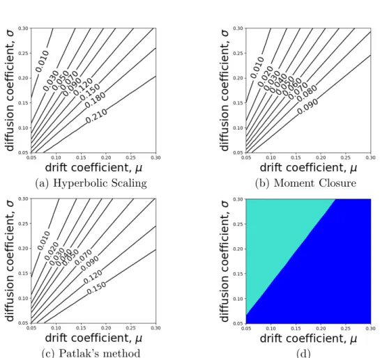
The movement kernel in Equation (2.32) contains two parameters, µand σ, hence I explore the parameter space to understand the impact of these parameters on the accuracy of approximations. The plots of contour lines of the KL-divergence on the µ−σ plane reveal that both the KL-divergence of u1I(x) from u1M(x) and the KL-divergence of u1I(x) from u1P(x) grow with increasing µ/σ (Figures
(a) Moment Closure (b) Patlak’s method
(c) 0.05≤µ≤0.2 , σ= 0.05 (d) µ= 0.05 , 0.05≤σ≤0.2
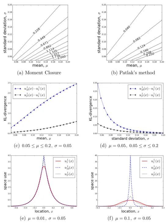
(e) µ= 0.01 , σ= 0.05 (f) µ= 0.1 , σ= 0.05 Figure 2.3: Discontinuous mean velocity movement kernelk1
τ(z|x) withµthe mean move length
in one step and σ the standard deviation of move length: The contours of the KL-divergence of the numerical solution, u1
I(x) , (a) from the analytic solution, u1M(x) (Equation 2.37), derived
using a moment closure technique, µ, σ ∈ [0.05,0.2] . (b) from the analytic solution, u1
P(x)
(Equation 2.40), derived using Patlak’s method, µ, σ∈[0.05,0.2] . (c) KL-divergence between
u1
M(x) and u1I(x) (N), and u1P(x) and u1I(x) (?) with 0.05 ≤ µ ≤ 0.2 and σ = 0.05 . (d)
KL-divergence between u1
M(x) and u1I(x) (N), and u1P(x) and u1I(x) (?) with 0.05≤σ≤0.2
and µ = 0.05 . (e) steady-state distributions with µ = 0.01 and σ = 0.05 . (f) steady-state distributions with µ= 0.1 and σ= 0.05 .
2.3a,b). Note that steady-state distribution u1H(x) equals to u1M(x) in this case (see Section 2.4.1).
Figures 2.3c,d show that the KL-divergence of u1I(x) from u1M(x) is greater than the KL-divergence of u1
I(x) from u1P(x), meaning u1P(x) is a better approximation
of u1
I(x). This implication is in opposition to the analytic analysis in Section 2.3,
which induces the conjecture that u1
M(x) might be closer to u1I(x) than u1P(x).
Nevertheless, neither of the two PDE methods captures the dynamics of the movement kernel properly. Both u1
M(x) and u1P(x) have sharp peaks at x = 0,
contrasting with the relatively smooth shape of u1
I(x), as shown in Figures 2.3e,f.
In addition, since µ/(σ2+µ2)< µ/σ2 for µ > 0, comparing Equations (2.37) and (2.40) reveals that u1P(0) < u1M(0) and the variance of u1P(x) is always greater than that of u1M(x) for µ > 0. This contributes to the smaller KL-divergence from u1
I(x) to u1P(x). That is, while all PDE techniques, including Patlak’s
approach, overestimate the probability density near the central place, Patlak’s approach also overestimate the variance, resulting in a flatter distribution closer to the real long-term distribution. However, note that the apparently greater variance of u1
P(x) observed in Figure 2.3f agrees with the analytic observations
of Section 2.3.
§2.5 A central-place foraging model with continuous mean velocity The movement kernel in Equation (2.32) in Section 2.4 describes movement to-wards an attraction centre with a fixed mean velocity, which is discontinuous at the central place, x = 0, as the direction changes. Results of analysing this movement kernel by the PDE methods show that there is a sharp spike in the steady-state distribution at the point where the mean velocity function is dis-continuous (Figures 2.3e,f). This sharp spike contrasts with the smooth shape of the actual long-term distribution derived from the ME in Equation (2.21). This means the distributions given by the PDE methods are very poor approximations to the actual long-term distribution. To understand how continuity of the mean velocity function affects the approximations, I consider another central-place for-aging model, where the mean velocity function is continuous over the real line.
Setting the central place at x= 0, the movement kernel studied here is kτ2(z|x) = 1 √ 2πσexp − (z−x−µ)2 2σ2 if x <−µ, 1 √ 2πσexp −z2 2σ2 if −µ≤x≤µ, 1 √ 2πσexp − (z−x+µ)2 2σ2 if x > µ. (2.41)
Here, the mean displacement over time τ is constant when the distance between the animal and the central place is greater than µ (i.e. |x−0|> µ), but equal to
|x| when the animal is located in the interval [−µ, µ], the vicinity of the central place.
2.5.1 Analysis of movement kernel kτ2(z|x) by the PDE techniques
When using the Hyperbolic Scaling and Moment Closure methods, the drift and diffusion coefficients are calculated by inserting the movement kernel in Equation (2.41) into Equations (2.4) and (2.5) to give
c2(x) = µ τ if x <−µ, −x τ if −µ≤x≤µ, −µ τ if x > µ, (2.42) and D2(x) = σ2 τ2. (2.43)
Here, the mean velocity function, c2(x), is continuous and the speed decreases as the animal approaches the central place when the distance to it is less than µ (Figure 2.4).
Although c2(x) is continuous, the derivative of c2(x) can only be defined piece-wise because c2(x) is not differentiable at points x=±µ. Therefore, I derive the steady-state distribution by substituting Equations (2.42) and (2.43) into Equa-tion (2.8) in three cases for x < −µ, −µ < x < µ and x > µ. Then assuming
Figure 2.4: An example of a continuous mean velocity function, defined by Equation (2.42), derived from a central-place foraging model with the central place being located at 0 (Equation 2.41).
continuity of the solution gives
u2H(x) = CH2 exp 2µ σ2x+ µ2 2σ2 if x <−µ, CH2 exp − 3 2σ2x 2 if −µ≤x≤µ, CH2 exp −2µ σ2x+ µ2 2σ2 if x > µ, (2.44) where CH2 = " σ2 µ exp −3µ 2 2σ2 + √ 2πσ √ 3 erf √ 3µ √ 2σ !#−1 (2.45) is a normalising constant ensuring that the distribution integrates to 1.
Applying the Moment Closure method to analyse the movement kernel in Equa-tion (2.41) is carried out in the same way. Placing EquaEqua-tions (2.42) and (2.43) into Equation (2.12) for x <−µ, −µ < x < µ and x > µ and assuming conti-nuity lead to the following steady-state distribution
u2M(x) = CM2 exp 2µ σ2x+ µ2 σ2 if x <−µ, CM2 exp −x 2 σ2 if −µ≤x≤µ, CM2 exp −2µ σ2x+ µ2 σ2 if x > µ, (2.46)
where CM2 = σ2 µ exp −µ 2 σ2 +√πσerfµ σ −1 (2.47) is a normalising constant. Here, since c2(x) (Equation 2.42) is non-constant for
−µ ≤ x ≤ µ and hence the derivative of c2(x) is non-zero on this interval, the integral in the steady-state solutions in Equations 2.8 and 2.12 are different on this interval. Consequently, the expressions for the solutions for −µ≤x≤ µ in Equations 2.44 and 2.46 are not the same and lead to different normalising terms (Equations 2.45 and 2.47).
To use Patlak’s approach, I calculate the first and second moments of displace-ment by placing the movedisplace-ment kernel in Equation (2.41) into Equations (2.14) and (2.15) to obtain M12(x) = µ if x <−µ, −x if −µ≤x≤µ, −µ if x > µ, (2.48) and M22(x) = ( σ2+µ2 if x <−µ orx > µ, σ2+x2 if −µ≤x≤µ. (2.49) Substitute Equations (2.48) and (2.49) into Equation (2.18) and assuming the distribution is continuous give the steady-state distribution derived by Patlak’s approach as follows: u2P(x) = CP2 (σ2+µ2)2 exp 2µ σ2+µ2x+ 2µ2 σ2 +µ2 if x <−µ, C2 P (σ2+x2)2 if −µ≤x≤µ, C2 P (σ2+µ2)2 exp − 2µ σ2+µ2x+ 2µ2 σ2 +µ2 if x > µ, (2.50) where CP2 = 1 µ(σ2+µ2) + arctan(µ/σ) σ3 + µ σ2(σ2+µ2) −1 (2.51) is a normalising constant.