Modeling Censored Data Using Mixture Regression
Models with an Application to Cattle Production Yields
Eric J. Belasco
Assistant Professor
Texas Tech University
Department of Agricultural and Applied Economics
eric.belasco@ttu.edu
Sujit K. Ghosh
Professor
North Carolina State University
Department of Statistics
Selected Paper prepared for presentation at the American Agricultural Economics Association Annual Meeting, Orlando, Florida, July 27 - 29, 2008
Copryright 2008 by Eric J. Belasco and Sujit K. Ghosh. All rights reserved. Readers may make verbatim copies of this document for non-commercial purposes by any means, provided that this copyright notice appears on all such copies.
Modeling Censored Data Using Mixture Regression Models with an
Application to Cattle Production Yields
Abstract:
This research develops a mixture regression model that is shown to have advantages over the classical Tobit model in model fit and predictive tests when data are generated from a two step process. Additionally, the model is shown to allow for flexibility in distributional assumptions while nesting the classic Tobit model. A simulated data set is utilized to assess the potential loss in efficiency from model misspecification, assuming the Tobit and a zero-inflated log-normal distribution, which is derived from the generalized mixture mdoel. Results from simulations key on the finding that the the proposed zero-inflated log-normal model clearly outperforms the Tobit model when data are generated from a two step process. When data are generated from a Tobit model, forecats are more accurate when utilizing the Tobit model. However, the Tobit model will be shown to be a special case of the generalized mixture model. The empirical model is then applied to evaluating mortality rates in commercial cattle feedlots, both independently and as part of a system including other performance and health factors. This particular application is hypothesized to be more apropriate for the proposed model due to the high degree of censoring and skewed nature of mortality rates. The zero-inflated log-normal model clearly models and predicts with more accuracy that the tobit model.
Modeling Censored Data Using Mixture Regression Models with an
Application to Cattle Production Yields
Censored dependent variables have long been a complexity associated with micro data sets. The most common occurrences are found in consumption and production data. Regarding con-sumption, households typically do not purchase all of the goods being evaluated in every time period. Similarly, a study evaluating the number of defects in a given production process will likely have outcomes with no defects. In both cases, ordinary least squares parameter estimates will be biased when applied to these types of regressions (Amemiya, 1984).
The seminal work by Tobin (1958) was the first to recognize this bias and offer a solution that is still quite popular today. The univariate Tobit model is extended, under a mild set of assump-tions, to include multivariate settings (Amemiya, 1974; Lee, 1993). While empirical applications in univariate settings are discussed by Amemiya (1984), multivariate applications are becoming more frequent (Belasco, Goodwin and Ghosh, 2007; Chavas and Kim, 2004; Cornick, Cox and Gould, 1994; Eiswerth and Shonkwiler, 2006). The assumption of normality has made the Tobit model inflexible to data generating processes outside of that major distribution (Bera et al., 1984). Additionally, Arabmazar and Schmidt (1982) demonstrate that random variables modeled by the Tobit model contain substantial bias when the true distribution is non-normal and has a high degree of censoring.
The Tobit model has been generalized to allow variables to influence the probability of a non-zero value and the non-zero value itself as two separate processes (Cragg, 1971; Jones, 1989), which are commonly referred to as the hurdle and double-hurdle models, respectively. Another model that allows for decisions or production output processes to be characterized as a two step process is the zero-inflated class of models.1
Lambert (1992) extended the classical ZIP model to include regression covariates, where covariate effects influence both ρ as well as the nonnegative outcome. Further, Li et al. (1999)
developed a multivariate zero-inflated Poisson model that is motivated to evaluate production pro-cesses involving multiple defect types. More recently, Ghosh et al. (2006) introduced a flexible class of zero-inflated models that can be applied to discrete distributions within the class of power series distributions. Their study also finds that Bayesian methods have more desirable finite sample properties than maximum likelihood estimation, with their particular model.
Computationally, a Bayesian framework may have significant advantages over classical meth-ods. In classical methods, such as maximum likelihood, parameter estimates are found through numerical optimization, which can be computationally intensive in the presence of many unknown parameter values. Alternatively, Bayesian parameter estimates are found by drawing realizations from the posterior distribution. Within large data sets the two methods are shown to be equivalent through the Bernstein-von Mises Theorem (Train, 2003). This property allows Bayesian methods to be used in place of classical methods, under certain conditions, which are asymptotically similar and may have significant computational advantages. In addition to asymptotic equivalence, Bayes estimators, in a Tobit framework, have been shown to converge faster than maximum likelihood methods (Chib, 1992).
In this study, we consider the use of a mixture model to characterize censored dependent variables as an alternative to the Tobit model. This model will be shown to nest the Tobit model, while major advantages include the flexibility in distributional assumptions and an increased effi-ciency in situations involving a high degree of censoring. For our empirical study, we derive the zero-inflated log-normal model from a generalized mixture model.
Data are then simulated to test the ability of each model to fit the data and predict out of
out by Gurmu and Trivedi (1996), hurdle and zero-inflated models can be thought of as refinements to models of truncation and censoring. Hurdle models typically use truncated-at-zero distributions, but are not restricted to truncated distributions. Cragg (1971) recommends the use of a log-normal distribution to characterize positive values. However, most applications of the hurdle model assume a truncated density function.
sample observations. Results from the zero-inflated mixture model will be compared to Tobit results through the use of goodness-of-fit and predictive power measures. By simulating data, the two models can be compared in situations where the data generating process is known.
In addition, a comprehensive data set will be used that includes proprietary cost and pro-duction data from five cattle feedlots in Kansas and Nebraska, amounting to over 11,000 pens of cattle during a 10 year period. Cattle mortality rates on a feedlot provide valuable insights into the profitability and performance of cattle on feed. Additionally, it is hypothesized that cattle mortality rates are more accurately characterized with a mixture model that takes into account the positive skewness of mortality rates, as well as allowing censored and non-censored observations to be modeled independently.2 In both univariate and multivariate situations, the proposed mixture model more efficiently characterizes the data.
Additionally, a multivariate setting is applied to these regression models by taking into ac-count other variables that describe the health and performance of feedlot cattle. These variables include dry matter feed conversion (DMFC), average daily gain (ADG), and veterinary costs per head (VCPH). Three unique complexities arise when modeling these four correlated yield mea-sures. First, the conditioning variables potentially influence the mean and variance of the yield dis-tributions. Since variance may not be constant across observations, we assume multiplicative het-eroskedasticity within our model and model conditional variance as a function of the conditioning variables. Second, the four yield variables are usually highly correlated, which is accommodated through the use of multivariate modeling. Third, mortality rates present a censoring mechanism where almost half of the fed pens contain no death losses prior to slaughter. This clustering of mass at zero presents biases when traditional least squares methods are used.
This paper provides two distinct contributions to existing research. The first is to develop a continuous zero-inflated log-normal model as an alternative modeling strategy to the Tobit model 2A zero-inflated specification is used rather than other mixture specifications, such as the Hurdle model, to more
and more traditional mixture models. This model will originate in a univariate case, then be ex-tended to allow for multivariate settings. The second contribution is to more accurately describe production risk for cattle feeders by examining model performance of different regression tech-niques. Mortality rates play a vital role in cattle feeding profits, particulary due to the skewed nature of this variable. A clearer understanding of mortality occurrences will assist producers as well as private insurance companies, who offer mortality insurance, in managing risk in cattle op-erations. Additionally, production risk in cattle feeding enterprises play a significant role in profit variability, but is currently uninsured by current federal livestock insurance programs. An accu-rate characterization of production risk plays an important role in addressing risk for producers or insurers.
The next section develops a generalized mixture model that is specified as a zero-inflated log-normal model and is used for estimation in this research. The univariate model will precede the development of a multivariate model. The following section simulates data based on the Tobit and given zero-inflated log-normal model to evaluate the loss in efficiency from model misspecifi-cation. This evaluation will consist of how well the model fits the data and the predictive accuracy. This will lead into an application where we evaluate data from commercial cattle feedlots in Kansas and Nebraska. Results from estimation using the Tobit and zero-inflated model will be assessed using both univariate and multivariate models. The final section provides the implications of this study and avenues of future research.
The Model
In general, mixture models characterize censored dependent variables as a function of two dis-tributions (Y =V B). First, B measures the likelihood of zero or positive outcomes, which have been characterized in the literature using Bernoulli and Probit model specifications. Then, the positive outcomes are independently modeled asV. A major difference between the mixture and
Tobit model is that unobservable, censored observations are not directly estimated. A generalized mixture model can be characterized as follows:
f(y|θ) = 1−ρ(θ) y=0
= ρ(θ)g(y|θ) y>0 (1)
whereR∞
0 g(y|θ)dy=1 ∀θ. This formulation includes the standard univariate Tobit model when
θ= (µ,σ),ρ(θ) =Φ µ σ , andg(y|θ) = φ( y−µ σ )
Φ(σµ) I(y>0). Notice that in the log-normal and Gamma
zero-inflated specifications to follow,ρis modeled independently of mean and variance parameter
estimates, making them more flexible than the Tobit model.
The above formulation may also be compared to a typical hurdle specification wheng(y|θ)is
assumed to be a zero-truncated distribution andρi(θ)is represented by a Probit model. The hurdle model as specified by Cragg (1971) is not limited to the above specification. In fact, the hurdle model can be generalized to include any standard regression model that takes on positive values for g(y|θ)and any decision model forρi(θ)that takes on a value between 0 and 1. In their generalized forms, both the hurdle and zero-inflated models appear to be similar, even though applications for each have differed.
Next, we develop two univariate zero-inflated models that include covariate variables, which then can be extended to allow for multivariate cases. Since only the positive outcomes are modeled through the second component, the log of the dependent variable can be taken. Taking the log of this variable works to symmetrize the dependent variable that was originally positively skewed. Using a log-normal distribution for theV random variable and allowing ρ to vary based on the
conditioning variables, we can transform the basic zero-inflated model into the following form that can be generalized to include continuous distributions. We start by deriving the normal distribu-tion to model the logarithm of the dependent variable outcomes, also known as the log-normal
distribution, of the following form f(yi|β,α,δ) = 1−ρi(δ) f or yi=0 = ρi(δ) 1 yiφ log(yi)−x0iβ σi otherwise (2) where ρi = 1 1+exp(x0iδ) (3) σ2i = exp(x0iα) (4)
which guarantees σ2i to be positive and ρi to lie between 0 and 1 for all observations and all parameter values. Notice that this specification is nested within the generalized version in equation (1) whereg(y|θ)is a log-normal distribution andθ= (δ,β,α).
In addition to deriving a inflated log-normal distribution, we will also derive a zero-inflated Gamma distribution to demonstrate the flexibility of the zero-zero-inflated regression models and perhaps improve upon modeling a variable that possesses positive skewness. Within a uni-variate framework, the sampling distribution can be easily changed by derivingV as an alternative distribution in much the same way as equation (2). Following is the specification for the zero-inflated Gamma distribution, where V is distributed as a Gamma distribution whereλiis the shape parameter, andηiis the rate parameter. This function can be reparameterized to include the mean of Gamma,µ, by substitutingλi=µiηi, whereηi=e(x
0
iκ)andµi=e(x0iγ). Within the Gamma
distri-bution specification, the expected value and corresponding variance can be found to beE(yi) =ρiµi andVar(yi) =ρi(1−ρi)µ2i +ρiηiµi, respectively. Both the Gamma and log-normal univariate spec-ifications allow for a unique set of mean and variance estimates to result from each distinct set of conditioning variables.
utilize the relationship between joint density and conditional marginal functions. More specifically, we utilize f(y1,y2) = f(y1|y2)f(y2) to capture the bivariate relationship when evaluatingy1 and y2, wherey1has a positive probability of taking on the value of 0 andy2is a continuous variable. In this case, f(y1,y2)is the joint density function ofy1andy2, f(y1|y2)is the conditional probability
ofy1, giveny2, and f(y2)is the unconditional probability ofy2. In order to compare this model to
that of the multivariate Tobit formulation, we derive a two-dimensional version ofy2, which can
easily be generalized to fit any size. However, this model restrictsy1to be one-dimensional under its current formulation.3
We begin by parameterizing, Z2i=log(y2), which will be distributed as a multivariate nor-mal, with mean,XiB(2), and variance,Σ22i. The assumption of log-normality is often made due to the ease in which a multivariate log-normal can be computed and its ability to account for skew-ness. This function can be expressed as Z2i∼N(XiB(2),Σ22i) where Z2i is an n x j dimensional matrix of positive outcomes. This formulation allows each observation to run through this mecha-nism, whereas the Tobit model runs only censored observations through this mechanism.
The conditional probability ofy1giveny2is modeled through a zero-inflated modeling mech-anism that takes into account the realizations fromy2such that
Y1|Y2=y2∼ZILN(ρi,µi(y2),σ2i(y2))where ZILN is a zero-inflated log-normal distribution,µi(y2)
is the conditional mean ofZ1i, which is defined asZ1i=log(y1), givenZ2i, andσ2i(y2)is the cor-responding conditional variance. More specifically,
µi(y2i) =XiB(1)+Σ12iΣ−221i
y2i−XiB(2)
andσ2i(y2i) =Σ11i−Σ12iΣ−221iΣ21i. This leads to the fol-lowing probability density function
3This will remain an area of future research. Deriving a model that allows for multiple types of censoring may be
very useful, particularly when dealing with the consumption of multiple goods. Using unconditional and conditional probabilities to characterize a more complex joint density function with multiple censored nodes would naturally extend from this modeling strategy.
f(Z1i|Z2i) = 1−ρi(δ) for y1i=0 = ρi(δ) 1 y1iφ Z1i−µi(y2i) q σ2i(y2i) for y1i>0 (5)
Ghosh et al. (2006) demonstrate through simulation studies that similar zero-inflated models have better finite sample performance with tighter interval estimates when using Bayesian pro-cedures instead of classical maximum likelihood methods. Due to these advantages, the previ-ously developed models will utilize recently developed Bayesian techniques. In order to develop a Bayesian model, the sampling distribution is weighted by prior distributions. The sampling distri-bution, f, is fundamentally proportional to the likelihood function,L, such thatL(θ|yi)∝ f(yi|θ)
where θ represents the estimated parameters, which for our purposes will include θ= (β,α,δ).
While prior assumptions can have some effects in small samples, this influence is known to di-minish with larger sample sizes. Additionally, prior assumptions can be uninformative in order to minimize any effects in small samples. For each parameter in the model, the following non-informative normal prior is assumed:
π(θ)∼N(0,Λ) (6)
such thatθ= (βk j,αk j,δkc)andΛ= (Λ1,Λ2,Λ3)fork=1, ...,K, j=1, ...,J, andc=1, ...,C, where
K is the number of conditioning variables or covariates, J is the number of dependent variables in the multivariate model, and C is the number of censored dependent variables.4 Additionally, Λ
must be large enough to make the prior relatively uninformative.5
Given the preceding specifications of a sampling density and prior assumptions, a full Bayesian 4The given formulation applies to univariate versions whenJ=1 andC=1.
5Λ is assumed to be 1,000 in this study, so that a normal distribution with mean 0 and variance 1,000 will be
model can be developed. Due to the difficulty in integrating a posterior distribution that contains many dimensions, Markov Chain Monte Carlo (MCMC) methods can be utilized to obtain sam-ples of the posterior distribution using WinBUGS programming software.6 MCMC methods allow for the computation of posterior estimates of parameters through the use of Monte Carlo simula-tion based on Markov chains that are generated a large number of times. The draws arise from a Markov chain since each draw depends only on the last draw, which satisfies the Markov property. As the posterior density is the stationary distribution of such a chain, the samples obtained from the chain are approximately generated from the posterior distribution following a burn-in of initial draws.
Predictive values within a Bayesian framework come from the predictive distributions, which is a departure from classical theory. In the zero-inflated mixture model, predicted values will be the product of two posterior mean estimates. Posterior densities for each parameter are com-puted from Markov Chain Monte Carlo (MCMC) sampling procedures using WinBUGS software. MCMC methods allow us to compute posterior density functions by sampling from the joint den-sity function that combines both the prior distributional information and the sampling distribution (likelihood function).7 Formally, prediction in the zero-inflated log-normal model is characterized by ˆyi=vibiwhereviandbiare generated from their predictive distributions.log(vi)is from a nor-mal distribution with mean (µi=x0iβˆ) and variance (σ2i =exp(x0iαˆ)), whilebi is from a Bernoulli distribution with parameter ρ(δˆ). Since many draws from a Bernoulli will result in 0 and 1
out-comes, the mean will produce an estimate that lies between the two values. To allow for prediction of both zero and positive values, the median of the Bernoulli draws was used for prediction, so that observations that contained more than 50% of 1 outcomes were given a 1 value and the rest were given 0. This allows for observations to fully take on the continuous random variable if more than 6Chib and Greenberg (1996) provide a survey of MCMC theory as well as examples of its use in econometrics and
statistics.
7WinBUGS will fit an appropriate sampling method to the specified model to obtain samples from the posterior
half of the time it was modeled to do so, while those that are more likely to take on zero values, as indicated by the Bernoulli outcomes, take on a zero value.
Comparison Using Simulated Data
This section will focus on simulating data in order to evaluate model efficiency for the two previ-ously specified models. The major advantage to evaluating a simulated set of data, is that the true form of the data generation process is known prior to evaluation. This will offer key insights into what to expect when evaluating an application involving the cattle production data set to follow. Additionally, we will evaluate data that come from Tobit and mixture processes, which will help to assess the degree of losses when the wrong type of model is assumed. This will assist in identify-ing the type of data that the cattle production data set most closely represents. In simulatidentify-ing data, there will be two key characteristics that will align the simulated data set with the cattle production data set to be used in the next section. First, cattle production yield variables have been shown to possess heteroskedastic errors. To accommodate this component error terms will be simulated based on a linear relationship with the conditioning variables. While the first set of simulations will consist of homoskedastic errors, the remaining simulations will use heteroskedastic errors. Second, we are concerned with simulated data that exhibit nearly 50% censoring to emulate the cattle production data set to be used as an application in the next section.
Past research has focused on modeling agricultural yields, while research dealing specifically with censored yields is limited. The main reason for the lack of research into censored yields is because crop yields are not typically censored at upper or lower bounds. However, with the emergence of new livestock insurance products, new yield measures must be quantified in order for risks to be properly identified. In contrast to crop yield densities, yield measures for cattle health possess positive skewness, such as the mortality rate and veterinary costs. Crop yield densities typically possess a degree of negative skewness as plants are biologically limited upward by a
maximum yield, but can be negatively impacted by adverse weather, such as drought. Variables such as mortality have a lower limit of zero, but can rise quickly in times of adverse weather, such as prolonged winter storms or disease. The simulated data set used for these purposes will possess positive skewness as well as a relatively high degree of censoring, in order to align with characteristics found in cattle mortality data for cattle on feed.
First, a simplified simulated data set will be examined with a varying number of observations. We assume in this set of simulations that that errors are homoskedastic. The simulated model will be as follows
y∗i = β0+β1x1i+β2x2i+εi (7)
εi ∼ N(0,σ2) (8)
yi = max(y∗i,0) (9)
In this scenario, the censored and uncensored variables come from the same data generation process.8 For each sample size, starting seeds were set in order to replicate results. Then, values forxiranged from 1 to 10, based on a uniform random distribution.9
Error terms are distributed as a normal, centered at zero with a constant variance set to σ.
y∗i is then computed from equation (7) and all negative values are replaced with zeros, in order to simulate a censored data set. The degree of censoring in these simulated data sets ranged from 49% to 62%.
While the first set of simulations provide a basis for evaluations, the assumptions of ho-moskedastic errors is a simplyfying assumption which has not been shown to hold in the applica-tion of cattle producapplica-tion yields. In order to more closely align with the given applicaapplica-tion, we now
8Simulated values are based on(β
0,β1,β2) = (2.0,3.7,−4.0)andσ2=1. 9Values forx
imight also be simulated using a normal distribution. A uniform distribution will more evenly spread
values ofxifrom the endpoints, while a normal distribution would cluster the values near a mean, without endpoints
(unless specified). Additionally, a uniform distribution will tend to result in fatter tails in the dependent variable due to the relatively high proportion of extreme values forxi.
move to simulate a data set containing heteroskedastic errors. Heteroskedasticity is introduced into this data by constructing εi by substituting equation (10) for equation (8) and accounting for the relationship between the error terms and the conditioning variables such that
εi ∼ N(0,σ2i) (10)
whereσ2i =exp(α0+α1x1i+α2x2i).10 These equations impose a dependence structure on the error term, where the variance is a function of the conditioning variables. This specification has been shown to better characterize cattle production yield measures (Belasco et al., 2006). Simulations were conducted in much the same manner as the previous set of simulations, with the addition of heteroskedastic errors.
Two thirds of this simulated data set is used for estimation, while the final third is used for prediction. This allows us to test both model fit measures as well as predictive power. In this study, Tobit regressions use classical maximum likelihood estimation techniques, while zero-inflated models use Bayesian estimation techniques. To derive measures of model fit we use the classical computation of Akaike’s Information Criteria (AIC) (Akaike, 1974) and derive a similar measure for Bayesian analysis, the Deviance Information criteria (DIC)(Spiegelhalter et al., 2002). DIC results are interpreted similar to AIC in that smaller values of the statistics reflect a better fit. A major difference is that AIC is computed based on the optimized value of the likelihood function where AIC=−2logL(βˆ,αˆ) +2P. In this case, P is the dimension of θ, which is 3 in the case
of homoskedastic errors and 6 with heteroskedastic errors. Alternatively, DIC is constructed by including prior information and is based on the deviance at the posterior means of the estimated parameters. A penalization factor for the number of parameters estimated is also incorporated into this measure. The formulation for DIC can be written as DIC=D¯ +pD where pD is the effective number of parameters and ¯Dis a measure of fit that is based on the posterior expectation of
10Simulated values are based on(α
deviance. These measures are specified as ¯D=E[−2logL(δ,β,α)|y]and pD=D¯+2logL(δ˜,β˜,α˜), which takes into account the posterior means, ˜δ, ˜β, and ˜α.
Robert (2001) reports that DIC and AIC are equivalent when the posterior distributions are approximately normal.11 Spiegelhalter et al. (2003) warns that DIC may not be a viable option for model fit tests when posterior distributions possess extreme skewness or bimodality. These concerns do not appear to be problematic in this study.
To measure the predictive power within a modeling strategy, we compute the Mean Squared Prediction Error (MSPE) associated with the final third of each simulated data set. MSPE allows us to test out of sample observations to assess how well the model predicts dependent variable values. MSPE is formulated as MSPE = m1∑mi=1(yˆi−yi)2 where m is some proportion of the full data sample, such thatm= nb. For our purposes,b=3, which allows for prediction on the final third, based on estimates from the first two thirds. This allows for a sufficient amount of observations available for estimation and prediction.
We estimate the simulated data set, given the above specifications, with the three models that have previously been formulated. MCMC sampling is used for Bayesian estimation with a burn-in of 1,000 observations and three Markov chains. WinBUGS uses different sampling methods, based on the form of the target distribution. For example, the zero-inflated Gamma distribution uses Metropolis sampling that fine tunes some optimization parameters for the first 4,000 iterations, which are not counted in summary statistics.
Results from Tobit regressions on the simulated data set with homoskedastic and heteroskedas-tic errors can be found in Table 1. Based on AIC/DIC criteria, the zero-inflated log-normal regres-sion model outperforms the Tobit model at all data sample levels. This is particularly interesting given the fact that simulation was based on a Tobit model. In cases where the degree of censoring is high, the parameter estimates that estimate the likelihood of censoring add more precision to the model. This impact is likely to diminish as the degree of censoring decreases and increases for
higher degrees of censoring.
The poor performance of the Gamma distribution highlights the problem associated with assuming an incorrect distribution. The Gamma distribution does particularly well with positive skewness, however, the degree of skewness in this model is not sufficient to overcome the incorrect distributional assumption.
Lower MSPE indicates that the prediction of the out of sample portion of the data set favors that of the Tobit model at all sample levels. MSPE penalizes observations with large residuals that tend to be more prevalent as the dependent variable value increases. Gurmu and Trivedi (1996) point out that mixture models tend to overfit data. By overfitting the data, model fit tests might improve, while prediction remains less accurate. This might explain part of the reason that mixture models appear to fit this particular set of simulated data better, while lacking prediction precision. Both zero-inflated models had particular trouble when predicting higher values ofy, resulting in high MSPE values. The wide spread of MSPE values is largely a result of simulating data that contains a high level of variability and a relatively small number of observations.
It is also important to point out that the Tobit model assumes positive observations are dis-tributed by a truncated normal distribution, while log-normal and Gamma distributions also take on only positive values but look very different than the truncated normal distribution. With roughly half of the sample censored, the density function from a truncated normal density would likely predict a larger mass near the origin, while the log-normal and Gamma distributions carry fatter tails.
As previously mentioned, another major difference between the hurdle and zero-inflated models in practice is the difference in modeling the binary decision variable using Probit and Bernoulli distributions, respectively. Based on the simulated data, the binary variables were com-puted using both methods did not appear to be significantly different.
As an alternative to the preceding simulation process, data can also be simulated using two separate data processes that emulate that of a mixture model more consistent with zero-inflated
models. The major distinction between this simulation and the previously developed Tobit-based data set, is that the probability of a censored outcome is modeled based on equation (3). Addi-tionally, outcomes that are described by a probability density function must be positive, which is achieved by taking the exponential of a normal distribution.12
Results from the second simulation can be found in Table 2. Once again, the results indicate a superior model fit with the zero-inflated model, relative to the Tobit model. Additionally, the zero-inflated models possess a substantially lower MSPE, indicating better out of sample prediction performance. Both zero-inflated formulations are capable of accounting for positive skewness. For the larger sample sizes, the Gamma formulation shows superior prediction ability, while the log-normal formulation is a better fit with the data. These results may come from the data generating process where the positive observations are generated from a log-normal distribution, however, the Gamma formulation predicts the outcomes that may come furthest from zero most accurately.
Accounting for both types of data generating processes, zero-inflated models are better able to fit data that contain a high degree of censoring. Prediction appears to depend on the data gener-ation process. If the data comes from a zero-inflated model, then prediction is more efficient when it is from a zero-inflated model. Alternatively, if all data comes from the same data generating process, then the Tobit may predict better than the proposed alternatives. One notable feature of the results generated from this simulation is that values for DIC appear to take on both positive and negative values. As mentioned previously, lower DIC/AIC indicate better fit measures. Therefore, a negative DIC is favorable to a positive AIC, which is the case under this scenario.
Most current research concerning censored data is focused on multivariate systems of equa-tions. This is because of the many applications that make use of multivariate relationships in
12This is the same as assumingy
iis distributed as a log-normal distribution. Alternatively, data could be generated
using a truncated normal distribution where simulations on a normal continues until all values are positive through iterations that spit out negative values and keep only positive values. The two methods would generate two very differ-ent data sets. Simulated values are based on values(β0,β1,β2) = (0.2,0.4,−0.6)and(δ0,δ1,δ2) = (−4.0,−5.0,7.0).
Additionallyσ2=1 and(α0,α1,α2) = (−0.2,0.1,−0.6)refer to homoskedastic and heteroskedastic simulations,
current studies. For this reason, it will be important to simulate a multivariate data set that comes from both a Tobit and a two-step process. Since multivariate data comes in both forms, it will be important to evaluate each to see the potential bias from assuming, for example, that data are generated from a multivariate Tobit model when a two-step process is more appropriate. The Tobit process is constructed from a multivariate normal distribution that assumes a specified covariance matrix. Censoring in this case occurs when the censored dependent variable falls below a specified level.13 Alternatively, the two-step process uses a Bernoulli distribution to estimate the likelihood of a censored outcome, which is also a function of the conditioning variables.14 To be consistent, the same variables that increase the likelihood of a censored outcome in the two-step case, also decrease the mean of the variable so that they increase the likelihood of a variable being censored in the Tobit process. Y1 andY2 are variables without censoring, whileY3 contains censoring in
nearly half of its observations.
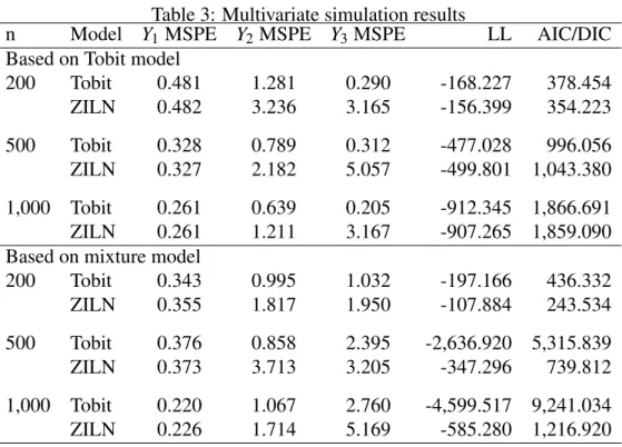
The results from a simulated data set based on a multivariate Tobit model are shown in Table 3. Overall, the fit of both models appear to be more closely aligned with the Tobit model in the first two simulations, while the zero-inflated model more accurately fits the model with the largest sample size. Additionally, the Tobit model predicts more efficiently, as shown by the lower MSPE in most cases. This is consistent with the univariate results and again is not surprising, given the data were generated from a Tobit model.
It is surprising the closeness of model fit, when we compare the results from data simulated from a mixture model, as shown in Table 3. Here, the zero-inflated model strongly improves the model fit, relative to the Tobit formulation. It is surprising that while most MSPE measures are close, they tend to favor the Tobit model formulation.
These simulations were conducted to compare the efficiency of the two given models in 13This method essentially simulates a system of equations that includes the latent variable, where the latent
variable is unobservable to the researcher. Simulated values were based onβ= (5,4,−1; 5,5,−1; 1,2,−2), α=
(−1.5,0.5,−1; 0.4,0.5,−1;−3, .5,−1), and cross products (t12,t13,t23)=(0.6,-0.4,0.3).
14Values for the simulation based on a multivariate mixture model were based on Tobit parameters with the addition
cases where the data are generated from a single data generating process, and that of a two-step process. Simulation results indicate that both models do relatively well in fitting the data, when the data come from a Tobit model. Alternatively, the model fit tests quickly move in the direction of the zero-inflated model in cases where the data comes from a mixture model and the non-zero observations are modeled using a multivariate log-normal distribution. Prediction of out of sample observations appear to be more efficiently characterized through the Tobit model. This is interest-ing given the fact that classical Tobit prediction uses only the optimized parameter values, while the zero-inflated model employs a Bayesian method that employs the entire posterior distribution of the estimated parameter values. Overall, the ZILN model tends to fit the data particularly well whether the data are generated from a Tobit or two-step process. This may result from the ad-ditional parameters that characterize the probability of a non-zero outcome in mixture models. However, this over-fitting does not assist in improving prediction, as prediction tends be more precise when the appropriate model is specified.
This section has offered some initial guidance into evaluating real data through the use of simulated data sets. The simulated data sets offer the opportunity to evaluate the performance of the Tobit and zero-inflated models in situations where the true data generation process is known. The next section will look to evaluate the same postulated models in an application where the true data generating process is unknown.
An Application
This section applies the preceding models to cattle production risk variables. The data set that will be used possesses many of the same properties from the last section, such as a relatively high degree of censoring and positive skewness in the dependent variables. The proposed zero-inflated log-normal model is hypothesized to characterize censored cattle mortality rates better than the Tobit model because of the two part process that mortality observations are hypothesized
to follow, as well as based on a visual inspection of positive mortality observations being more closely characterized by a log-normal distribution. Cattle mortality rates are thought to follow a two step process because pens tend to come from the same, or nearby, producers and are relatively homogenous. Therefore, a single mortality can be seen as a sign that a pen that is more prone to sickness or disease. Additionally, airborne illnesses are contagious and can be spread rather quickly throughout the pen. Other variables that describe cattle production performance are introduced and evaluated using the previously developed multivariate framework. These variables include DMFC, which is measured as the average pounds of feed a pen of cattle require to add a pound of weight gain, and ADG, which is the average daily weight gain per head of cattle. VCPH is the amount of veterinary costs per head that are incurred over the feedlot stay.
This research focuses on the estimation and prediction of cattle production yield measures. Cattle mortality rates from commercial feedlots are of particular interest due to their importance in cattle feeding profits. Typically, mortality rates are zero or small, but can rise significantly during adverse weather, illness, or disease. The data used in this study consists of 5 commercial feedlots residing in Kansas and Nebraska, and includes entry and exit characteristics of 11,397 pens of cattle at these feedlots. Table 4 presents a summary of characteristics for different levels of mortality rates, including no mortalities
Particular attention will be placed on whether zero or positive mortality rates can be strongly determined based on the data at hand. The degree of censoring in this sample is 46%, implying that almost half of the observations contain no mortality losses. There is strong evidence that mortality rates are related to the previously mentioned conditioning variables, but we will need to determine whether censored mortality observations are systematically different than observed positive values. Positive mortality rates may be a sign of poor genetics coming from a particular breeder or sickness picked up within the herd. The idea here is that the cattle within the pen are quite homogeneous. Homogeneity within the herd is desirable as it allows for easier transport, uniform feeding rations, medical attention, and the amount of time on feed. If homogeneity within the herd holds, then pens
that have mortalities can be put into a class that is separate from those with no mortalities.
However, mortalities also may occur without warning and for unknown reasons. Glock and DeGroot (1998) report that 40% of all cattle mortalities in a Nebraska feedlot study were directly caused by Sudden Death Syndrome.15 However, the authors also point out that these deaths were without warning, which could be due to a “sudden death” or lack of observation by the feedlot workers. Smith (1998) also reports that respiratory disease and digestive disorders are responsible for approximately 44.1% and 25.0% of all mortalities, respectively. The high degree of correlation between dependent variables certainly indicates that lower mortality rates can be associated with different performance in the pen. However, the question in this study will be whether positive mortality rates significantly alter the performance. For this reason, we estimate additional parameters to examine the likelihood of a positive mortality outcome in the zero-inflated regression model.
A recent study by Belasco et al. (2006) found that the mean and variance of mortality rates in cattle feedlots are influenced by entry-level characteristics such as location of the feedlot, place-ment weight, season of placeplace-ment and gender. These variables will be used as conditioning vari-ables. By taking these factors into account, variations will stem from events that occur during the feeding period as well as characteristics that are unobservable in the data. The influence of these parameters will be estimated using the previously formulated models, based on two-thirds of the randomly selected data set where n=7,598. The remaining portion of the data set, m=3,799, will be used to test out of sample prediction accuracy. Predictive accuracy is important in existing crop insurance programs where past performance is used to derive predictive density functions for current contracts.16
After estimating expected mortality rates, based on pen-level characteristics, we will focus 15Glock and DeGroot (1998) loosely define Sudden Death as any case where feedlot cattle are found dead
unex-pectedly.
16The most direct example of this is the Average Production History (APH) crop insurance program that insures
our attention to estimating mortality rates as part of a system of equations that includes other per-formance and health measures for fed cattle, such as dry matter feed conversion (DMFC), average daily gain (ADG), and veterinary costs (VCPH), which are additional measures of cattle production yields.
Estimation Results
A desireable model specification will be one that fits the data in estimation and is able to predict dependent variable values with accuracy. For these reasons, these models will be compared in a way similar to the simulated data sets. First, we begin with univariate results. Results from using a classical Tobit model with heteroskedastic errors to model cattle mortality rates can be found in Table 5.
Tobit estimates forβmeasure the marginal impact of changes in the conditional variables on
the latent mortality rate.17 For example, the coefficient corresponding to in-weight, states that a 10% increase in entry weight lowers the latent variable by 3.9%.18 The estimates for αmeasure
the relative impact on the variance. For example, the estimation coefficient corresponding to fall implies that a pen placed in that period is associated with a variance that is 32% higher than the base months containing summer. MSPE is computed as the average squared difference between the predicted and actual mortality rates.
Next, we move to estimate the same set of data using the previously developed zero-inflated models in order to test our hypothesis that they will have a better fit. Before proceeding to es-timation, there are a few notable differences when using classical and Bayesian methods. First, 17The Tobit specification assumes that the latent variable is a continuous, normally distributed variable that is
ob-served for positive values and zero for negative values. Marginal changes in the latent variable must then be converted to the marginal changes in the observed variable, in order to offer inferences on the observable variable. The marginal impact on mortality rates can be approximated by multiplying the marginal impact on the latent variable by the degree of censoring (Greene, 1981)
18McDonald and Moffitt (1980) show how Tobit parameter estimates can be decomposed into two parts, where the
first part contains the effect on the probability that the variable is above zero, while the second part contains the mean effect, conditional on being greater than zero.
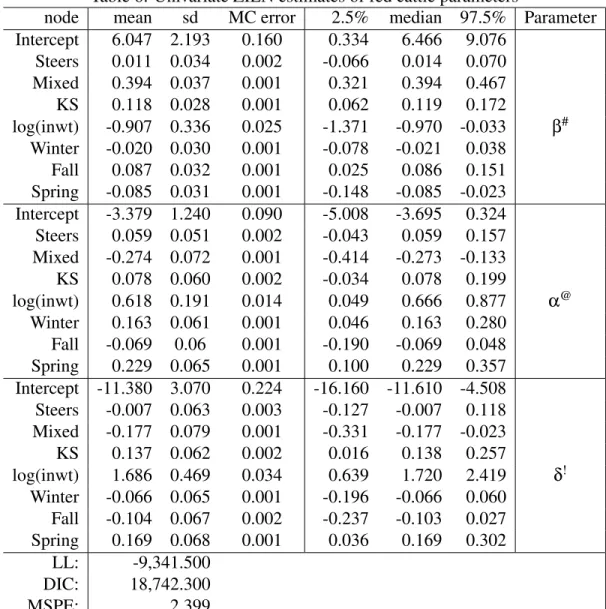
Bayesian point estimates are typically computed as the mean from Monte Carlo simulations of the posterior density function. This estimation process is done in two parts; first the likelihood of a zero value is modeled, followed by simulating the positive predicted realizations, based on a log-normal distribution. In addition to the mean value, additional characteristics of the posterior distributions are supplied, such as the median, 2.5 and 97.5 percentile values, and the standard deviation, as well as the Monte Carlo standard error of the mean. Results from the zero-inflated log-normal model are shown below in Table 6.
Parameter estimates in the zero-inflated model refer to two distinct processes. The first process includes the likelihood of a zero outcome or one described by a log-normal distribution. This process is estimated throughδutilizing equation (3). Based on this formulation, the parameter
estimates can be expressed as the negative of the marginal impact of the conditional variable on the probability of a positive outcome, relative to the variance of the Bernoulli component:
δk=− ∂ρi ∂xki · 1 ρi · 1+exp(x0iδ) exp(x0iδ) =−∂ρi ∂xki · 1 ρi(1−ρi) (11)
where the variance is shown asρi(1−ρi). For example, entry weight largely and negatively influ-ences the likelihood of positive mortality rates. This is not surprising given that more mature pens are better equipped to survive adverse conditions, whereas younger pens tend to be more likely to result in mortalities. Alternatively, mixed pens have a negativeδcoefficient which implies that
there is a positive relationship, relative to heifer pens. Therefore, if a pen is mixed, it has a higher probability of incurring positive mortality realizations that can be modeled with a log-normal dis-tribution.
The Tobit model assumes that estimates forβ andδ will work in the same way. For most
variables, δ coefficients are negatively related to βcoefficients, which points to directional
con-sistency. For example, increases to entry weight shift the mean of mortality rates downward and also decrease the probability of a positive outcome. This does not necessarily mean that the two
processes work identically, as is assumed with the Tobit model, but rather tend to generally work in the same direction.
Parameter estimates forβ refer to the marginal impact that the conditioning variables have
on the positive realizations of mortality rates. Interpretations for these parameters refer to the marginal increase in the log of mortality rate. For example, an increase in entry weight by 1.0% is associated with a reduction in mortality rates by 0.9% for the observations that experience a positive mortality rate.
It is interesting to note the different implications from parameter estimates from the Tobit and ZILN models. For example, an insignificant mean parameter estimate for the variable KS in the Tobit model implies that mortality rates are not significantly impacted by feedlot location. However, parameter estimates from the ZILN model infer that pens placed into feedlots located in Kansas have a lower likelihood of a positive mortality realization by 13.7%, relative to Nebraska feedlots. At the same time, pens placed in Kansas that have a positive mortality rate, can be expected to realize a rate that is 11.8% higher than Nebraska feedlots. This might seem strange to have significant impacts in opposite directions that influence both the likelihood of a mortality and the positive mortality rate, but by distinguishing between these processes we can isolate their respective impacts. One possible explanation might be that Kansas lots spend more time to prevent mortalities from occurring through vaccinations or backgrounding, but are not able to prevent the spread of disease as quickly as the Nebraska feedlots. This is a notable departure from the Tobit model which saw no significant influence since these impacts essentially canceled each other out.
Another notable difference is in seasonal impacts on the mean of mortality rates. While the none of the seasonal variables are significantly different than summer under the Tobit model, both Fall and Spring are significantly different under the ZILN specification. The ZILN results are more inline with expectations as Fall placement are put under stress from extremely cold weather, which is different from summer placements. In fact, most of the pens with mortality losses above 10% in this data sample come from pens placed in the fall months.
The zero-inflated log-normal models also demonstrate a superior ability to characterize and predict cattle feedlot observations. A DIC measure of 18,742.3 demonstrates a closer fit, relative to the Tobit model, which as an AIC value of 22,790.7. Additionally, MSPE is minimized when using the ZILN model. The likely explanation for these findings is due to the data generating process. Cattle mortalities appear to be part of a two part process where once a pen experiences a mortality, the rate of mortalities can be modeled using a distinct distribution from those observations without mortalities.19
The given data set was also modeled using a zero-inflated Gamma (ZIG) distribution. While the Bernoulli component is similar to the ZILN model, this model characterizes the positive ob-servations using a Gamma distribution, which also can take into account highly skewed data. The results from the ZIG model are shown below in Table 7.
Regressions from univariate mortality models offer information concerning the relative im-pacts each conditioning variable has on mortality rates. However, this variable is likely better characterized in a multivariate setting with other variables that explain the health and performance of cattle on feedlots, ultimately describing production risk in cattle feeding enterprises. To this end, the multivariate Tobit model and multivariate zero-inflated models were used to characterize these four variables, described earlier. The results from the multivariate Tobit model are shown in table 8.
Results from this estimation mostly appear to be in line with the estimation from Belasco et al. (2006), as well as the first essay. While the same data set was used, this study employs two-thirds of the data for estimation and the final third for out of sample prediction. Mortality rates contain the most variability in prediction, mostly due to the relative lack of explanatory power from 19This method may also be useful in situations where the data have some similar characteristics. Examples may be
modeling the prevalence of animal disease, where a Bernoulli distribution characterizes the likelihood of an outbreak. Once an outbreak has occurred, a model describing its biological spread is needed. This strategy may also extend into areas of bio-security and food safety issues where biological processes may be allowed to spread within a population once contamination has occurred. Additionally, data that are characterized with a high degree of censoring can be efficiently characterized through the use of a zero-inflated model, as shown in earlier simulations.
the conditioning variables. While theseex-ante variables offer information on expected mortality rates, there does still appear to be a bit more unexplained variation than with the other variables. Performance variables, such as DMFC and ADG, are largely determined by observable biological traits. While not all of these biological traits are captured in these data, there does not appear to be a large portion unexplained by these variables.
The elements contained within the covariance matrix are under the estimates labeled as ’Het-eroskedasticity’.20 The sign of the off-diagonal covariance elements describe the relationship be-tween two variables. For example, DMFC and ADG are negatively related with a coefficient of -4.09, since a healthy pen of cattle will be expected to have a low feed conversion rate and a high rate of gain. Additionally, MSPE is broken out by dependent variable. MORT has the highest MSPE, which illustrates the lack of predictive power with that variable.
Next, the multivariate zero-inflated model is applied to the cattle feedlot data set and results are shown in Table 9. Estimates displayed here are consolidated, relative to the univariate table due to space constraints. In a Bayesian framework, confidence intervals are typically computed using the highest posterior density region, which will be different from a classical confidence interval when posterior distributions are bi-modal or asymmetric. Since the posterior estimates do not show bi-modal attributes, we proceed by taking the interval between the 2.5 and 97.5 percentiles to test whether the variable is significantly different from zero. While this is a departure from Bayesian theory, it nearly aligns with significance tests for the multivariate Tobit model. For example, in the zero-inflated model, if the posterior density function does not cross zero in the given interval, which includes 95 percent of the posterior density, then it is said to be significant at the 5% level.
Many of the same estimates appear in the zero-inflated table, with the addition of ’Delta’ terms, which describe the negative of the relative impact on the probability of a non-zero outcome. These estimates are computed in the same way as the univariate version of this model, leading to 20Belasco et al. (2007) provide a more detailed discussion concerning the construction of the covariance matrix for
many of the same inferences. Additionally, parameter estimates corresponding to DMFC, ADG, and VCPH are mostly the same between the Tobit model and ZILN models. Parameter estimates corresponding to MORT are different between the two models, as discussed with the univariate model.
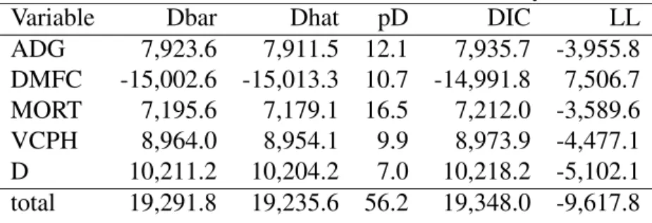
The zero-inflated model does a superior job of fitting the data and in terms of prediction accuracy, relative to the Tobit model. DIC for the ZILN model is substantially lower than AIC in the Tobit model, mainly due to the more accurate fit for Mortality rates, which contributes quite a lot of unexplained variability to the system of equations. The more efficient modeling of mortality rates stem from the ability of the zero-inflated model to more accurately represent MORT by taking into account the two part process inherent in mortality rates. MSPE measures are approximately the same for each of the non-censored variables, largely because they are modeled in a similar fashion. However, more information about mortality rates in the zero-inflated model add to more accurately model the other variables. In fact, the multivariate zero-inflated model predicts every dependent variable with more precision, leading to large gains in both prediction and model fitting. We can decompose the total DIC and LL values from the multivariate zero-inflated model into dependent variable components, which is shown in Table 10.21 This table is helpful in breaking down model fit measures to identify the performance of the model on each variable. MORT is more accurately characterized in a multivariate setting because of the effects from other non-censored variables. Recall, that the expected value and variance of MORT accounts for the uncensored variable levels in the multivariate setting. D represents the estimation on the parameters of ’Delta’, which performs roughly similar in both multivariate and univariate situations, since it uses the same modeling mechanism in each case. DMFC is modeled very tightly, as shown by the negative DIC, while ADG and VCPH leave some variability unestimated. The results from the total line are reported with the full model results in Table 9.
21LL values are computed by dividing Dhat by -2, sinceDhat=−2∗LL(βˆ,γˆ,δˆ). This aligns with LL values in the Tobit model which are computed based on optimized values. Along the same lines, Dhat is computed by using the optimal posterior means.
Implications and Recommendations
Modeling censored data remains a large area of concern and current research in econometrics. While use of the Tobit model may be well-justified in certain instances, the results from both simulated and actual cattle feeder data sets suggest the use of a zero-inflated modeling mechanism. This is particularly true in instances where data come from a two-step process. While two-step processes have been applied to hurdle models, zero-inflated models have largely been ignored in economic studies. This is mainly a result of the past limitation of zero-inflated models to count data. In this study, a mixture model is developed that can handle both univariate and multivariate situations rather efficiently, in addition to nesting the standard Tobit model. Additionally, the inherent parametric flexibility allows for distributional assumptions to change based on the data on hand, rather than strictly using truncated or normally distributions. Here we use a log-normal distribution to capture the positively skewed nature of cattle feedlot mortality rates, which gives the zero-inflated log-normal model significant advantages over the Tobit model. Advantages in model fit for the ZILN model stem from the ability to isolate and identify the impacts from observing a positive mortality rate and the level of mortality rates. However, the Tobit model is also shown to be a special case of the general mixture model.
Production risk in cattle feeding enterprises is inherently complex, given the many areas risk can originate. Results from this research demonstrate the potential gains from using this particular mixture model. Before applying this model to the data, simulations were conducted to test the model’s ability to predict and fit data generated in different forms. These simulations provide results that support the use of the mixture model, in both prediction and model fit, when the data is from a two-step process. Additionally, the mixture model demonstrated a strong ability to fit the data, even when the data are generated based on a Tobit model. These results are in general agreement with the results obtained within our application of cattle feeding.
vari-ability. The proposed model takes a step forward in developing a modeling strategy that can be used to measure other livestock or live animal productive measures. By more accurately charac-terizing these risks insurance companies, animal producers, and operators can better understand the risks involved with animal production. Future research is currently focusing on developing this model to account for systems where censoring occurs in more than three variables, which is cur-rently problematic in classical estimation techniques. Examples where this particular model might be useful include consumption, livestock disease spread, or production processes.
Additionally, the flexibility of this model allows for uses outside of live animal yields. The major flexibility in the proposed model lies in the ability to make different distributional assump-tions. Distributional assumptions typically need to be made in cases when data cannot fully explain variability. However, nonparametric and semi-parametric methods may be of particular interest when large data sets are evaluated, since they allow empirical data to create a unique density. With more data available on live animal yields, augmenting this model to include these types of density functions may provide additional precision.
References
Akaike, H. (1974) ‘A new look at the statistical model identification.’IEEE Transactions on Auto-matic Control19, 716–723
Amemiya, T. (1974) ‘Multivariate regression and simultaneous equation models when the depen-dent variables are truncated normal.’Econometrica42(6), 999–1012
(1984) ‘Tobit models: A survey.’Journal of Econometrics24, 3–61
Arabmazar, A., and P. Schmidt (1982) ‘An investigation of the robustness of the tobit estimator to non-normality.’Econometrica50(4), 1055–1064
Belasco, E. J., B. K. Goodwin, and S. K. Ghosh (2007) ‘A multivariate evaluation of ex-ante risks associated with fed cattle production.’ Selected Paper. SCC-76: Economics and Management of Risk in Agriculture and Natural Resources Annual Meeting
Belasco, E. J., M. R. Taylor, B. K. Goodwin, and T. C. Schroeder (2006) ‘Probabilistic models of yield, price, and revenue risk for fed cattle production.’ Selected Paper. American Agricultural Economics Association Annual Meeting, Long Beach
Bera, A. K., C. M. Jarque, and L. F. Lee (1984) ‘Testing the normality assumption in limited dependent variable models.’International Economic Review25(3), 563–578
Chavas, J. P., and K. Kim (2004) ‘A heteroskedastic multivariate tobit analysis of price dynamics in the presence of price floors.’American Journal of Agricultural Economics86(3), 576–593
Chib, S. (1992) ‘Bayes inference in the tobit censored regression model.’Journal of Econometrics 51, 79–99
Chib, S., and E. Greenberg (1996) ‘Markov chain monte carlo simulation methods in econometric.’ Econometric Theory12(3), 409–431
Cornick, J., T. L. Cox, and B. W. Gould (1994) ‘Fluid milk purchase: A multivariate tobit analysis.’ American Journal of Agricultural Economics76, 74–82
Cragg, J. G. (1971) ‘Some statistical models for limited dependent variables with application to the demand for durable goods.’Econometrica39(5), 829–844
Eiswerth, M. E., and J. S. Shonkwiler (2006) ‘Examining post-wildfire reseeding on arid range-land: A multivariate tobit modeling approach.’Econological Modeling192, 286–298
Ghosh, S. K., P. Mukhopadhyay, and J. C. Lu (2006) ‘Bayesian analysis of zero-inflated regression models.’Journal of Statistical Planning and Inference136, 1360–1375
Glock, R. D., and B. D. DeGroot (1998) ‘Sudden death of feedlot cattle.’Journal of Animal Science 76, 315–319
Greene, W. H. (1981) ‘On the asymptotic bias of the ordinary least squares estimator of the tobit model.’Econometrica49(2), 505–513
Gurmu, S., and P. K. Trivedi (1996) ‘Excess zeros in count models for recreation trips.’Journal of Business and Economic Statistics14(4), 469–477
Jones, A. M. (1989) ‘A double-hurdle model of cigarette consumption.’Journal of Applied Econo-metrics4(1), 23–39
Lambert, D. (1992) ‘Zero-inflated poisson regression, with an application to defects in manufac-turing.’Technometrics34(1), 1–14
Lee, L. F. (1993) ‘Multivariate tobit models in econometrics.’ InHandbook of Statistics, Vol. 11, ed. G. S. Maddala, C. R. Rao, and H. D. Vinod. chapter 6, pp. 145–173
Li, C. S., J. C. Lu, J. Park, K. Kim, P. A. Brinkley, and J. P. Peterson (1999) ‘Multivariate zero-inflated poisson models and their applications.’Technometrics41(1), 29–38
McDonald, J. F., and R. A. Moffitt (1980) ‘The uses of tobit analysis.’ The Review of Economics and Statistics62(2), 884–895
Robert, Christian P. (2001)The Bayesian Choice: from decision-theoretic foundations to compu-tational implementation,2nd ed. (Springer texts in statistics)
Smith, R. A. (1998) ‘Impact of disease on feedlot performance: A review.’ Journal of Animal Science76, 272–274
Spiegelhalter, D., A. Thomas, N. Best, and D. Lunn (2003) ‘Winbugs user manual, version 1.4 mrc biostatistics unit, cambridge, uk.’ http://www.mrc-bsu.cam.ac.uk/bugs
Spiegelhalter, D. J., N. G. Best, B. P. Carlin, and A. van der Linde (2002) ‘Bayesian measures of model complexity and fit.’Journal of the Royal Statistical Association, Series B64, 583–639
Tobin, J. (1958) ‘Estimation of relationships for limited dependent variables.’ Econometrica 26(1), 24–36
Table 1: Simulation results based on Tobit model
n Model MSPE LL AIC/DIC
Homoskedastic errors 200 Tobit 0.773 -86.044 184.088 ZILN 23.982 -58.162 122.934 ZIG 4.453 -165.280 337.138 500 Tobit 0.460 -258.590 529.179 ZILN 96.064 -170.905 350.238 ZIG 52.720 -497.998 1,002.490 1,000 Tobit 0.466 -508.902 1,029.805 ZILN 94.809 -400.526 809.331 ZIG 47.098 -985.960 1,977.590 Heteroskedastic errors 200 Tobit 16.624 -87.057 186.114 ZILN 20.416 -57.162 123.416 ZIG 17.083 -187.151 381.949 500 Tobit 6.205 -248.387 508.774 ZILN 10.156 -168.842 348.661 ZIG 12.018 -546.32 1,100.390 1,000 Tobit 10.012 -453.739 919.478 ZILN 14.528 -358.822 728.513 ZIG 16.745 -1,024.810 2,058.140
Table 2: Simulation results based on mixture model
n Model MSPE LL AIC/DIC
Homoskedastic errors 200 Tobit 1.953 -95.535 203.069 ZILN 0.280 -2.583 11.510 ZIG 0.303 6.905 -7.865 500 Tobit 2.153 -276.410 564.821 ZILN 0.079 29.148 -50.412 ZIG 0.083 13.379 -20.674 1,000 Tobit 1.189 -499.676 1,011.351 ZILN 0.044 21.211 -33.565 ZIG 0.046 82.563 -158.735 Heteroskedastic errors 200 Tobit 77.813 -40.024 92.049 ZILN 63.386 -26.204 60.732 ZIG 64.052 -76.506 160.651 500 Tobit 12.941 -130.961 273.923 ZILN 4.303 -102.802 214.994 ZIG 3.971 -235.094 478.824 1,000 Tobit 4.610 -272.204 556.407 ZILN 2.948 -183.034 376.549 ZIG 2.468 -430.032 867.893
Table 3: Multivariate simulation results
n Model Y1MSPE Y2MSPE Y3MSPE LL AIC/DIC Based on Tobit model
200 Tobit 0.481 1.281 0.290 -168.227 378.454 ZILN 0.482 3.236 3.165 -156.399 354.223 500 Tobit 0.328 0.789 0.312 -477.028 996.056 ZILN 0.327 2.182 5.057 -499.801 1,043.380 1,000 Tobit 0.261 0.639 0.205 -912.345 1,866.691 ZILN 0.261 1.211 3.167 -907.265 1,859.090 Based on mixture model
200 Tobit 0.343 0.995 1.032 -197.166 436.332 ZILN 0.355 1.817 1.950 -107.884 243.534 500 Tobit 0.376 0.858 2.395 -2,636.920 5,315.839 ZILN 0.373 3.713 3.205 -347.296 739.812 1,000 Tobit 0.220 1.067 2.760 -4,599.517 9,241.034 ZILN 0.226 1.714 5.169 -585.280 1,216.920
Table 4: Comparison of pens with differing mortality losses Mortality Rate (%)a Variable 0 0.01 - 1 1 - 2 2 - 3 3 - 4 >4 Observations 5,161 2,415 2,327 744 305 445 DMFC 6.05 6.27 6.21 6.34 6.42 6.85 ADG 3.49 3.35 3.28 3.11 3.06 2.82 Intake 20.96 20.82 20.15 19.52 19.49 18.88 VCPH 10.18 10.08 12.46 15.67 17.89 26.57 InWt 754.27 751.53 719.72 686.35 699.00 671.63 OutWt 1,188.72 1,179.90 1,168.75 1,152.95 1,158.40 1,144.66 HeadIn 120.24 182.04 126.19 123.14 114.72 110.57 Days on Feed 123.45 125.66 133.44 143.83 141.57 150.57 Proportion of sample: Winter 0.24 0.27 0.26 0.29 0.29 0.21 Spring 0.26 0.24 0.21 0.16 0.17 0.10 Summer 0.27 0.26 0.26 0.25 0.24 0.30 Fall 0.23 0.23 0.27 0.30 0.30 0.39 Steers 0.53 0.56 0.49 0.43 0.42 0.35 Heifers 0.36 0.37 0.37 0.36 0.38 0.33 Mixed 0.10 0.07 0.14 0.20 0.20 0.32 KS 0.82 0.76 0.82 0.77 0.79 0.82
aNote: A mortality rate that results in a whole number is placed into the higher bins
Table 5: Univariate Tobit estimates of fed cattle mortality parameters
β# α@
Variables coeff. se. coeff. se Intercept: 25.782∗ 1.515 12.068∗ 1.114 Steers: 0.168∗ 0.055 -0.021 0.048 Mixed: 0.307∗ 0.124 0.984∗ 0.073 Kansas: -0.068 0.058 0.292∗ 0.058 log(inwt): -3.893∗ 0.231 -1.654∗ 0.172 Winter: 0.065 0.068 -0.243∗ 0.061 Fall: 0.043 0.079 0.315∗ 0.061 Spring: -0.089 0.069 -0.278∗ 0.065 LL: -11,389.353 AIC: 22,790.706 MSPE: 2.661
∗Denotes estimate is significant at the 0.05 level #βmeasures the marginal change on the mean
of the latent variable
@
Table 6: Univariate ZILN estimates of fed cattle parameters
node mean sd MC error 2.5% median 97.5% Parameter Intercept 6.047 2.193 0.160 0.334 6.466 9.076 Steers 0.011 0.034 0.002 -0.066 0.014 0.070 Mixed 0.394 0.037 0.001 0.321 0.394 0.467 KS 0.118 0.028 0.001 0.062 0.119 0.172 log(inwt) -0.907 0.336 0.025 -1.371 -0.970 -0.033 β# Winter -0.020 0.030 0.001 -0.078 -0.021 0.038 Fall 0.087 0.032 0.001 0.025 0.086 0.151 Spring -0.085 0.031 0.001 -0.148 -0.085 -0.023 Intercept -3.379 1.240 0.090 -5.008 -3.695 0.324 Steers 0.059 0.051 0.002 -0.043 0.059 0.157 Mixed -0.274 0.072 0.001 -0.414 -0.273 -0.133 KS 0.078 0.060 0.002 -0.034 0.078 0.199 log(inwt) 0.618 0.191 0.014 0.049 0.666 0.877 α@ Winter 0.163 0.061 0.001 0.046 0.163 0.280 Fall -0.069 0.06 0.001 -0.190 -0.069 0.048 Spring 0.229 0.065 0.001 0.100 0.229 0.357 Intercept -11.380 3.070 0.224 -16.160 -11.610 -4.508 Steers -0.007 0.063 0.003 -0.127 -0.007 0.118 Mixed -0.177 0.079 0.001 -0.331 -0.177 -0.023 KS 0.137 0.062 0.002 0.016 0.138 0.257 log(inwt) 1.686 0.469 0.034 0.639 1.720 2.419 δ! Winter -0.066 0.065 0.001 -0.196 -0.066 0.060 Fall -0.104 0.067 0.002 -0.237 -0.103 0.027 Spring 0.169 0.068 0.001 0.036 0.169 0.302 LL: -9,341.500 DIC: 18,742.300 MSPE: 2.399 #
βmeasures the marginal change on the mean of the latent variable
@αmeasures the relative impact on the variance
Table 7: Univariate ZIG estimates of fed cattle parameters
node mean sd MC error 2.5% median 97.5% Parameter Intercept 2.569 0.424 0.031 1.904 2.510 3.350 Steers -0.054 0.033 0.002 -0.115 -0.054 0.010 Mixed 0.379 0.044 0.002 0.295 0.379 0.466 KS 0.014 0.034 0.002 -0.054 0.015 0.079 log(inwt) -0.410 0.066 0.005 -0.533 -0.402 -0.310 γ Winter 0.035 0.040 0.002 -0.040 0.034 0.118 Fall 0.134 0.040 0.002 0.057 0.133 0.217 Spring -0.188 0.044 0.002 -0.270 -0.190 -0.094 1.187 0.028 0.001 1.134 1.187 1.243 κ Intercept -0.465 0.427 0.031 -1.426 -0.429 0.318 Steers 0.114 0.052 0.003 0.010 0.113 0.221 Mixed -0.168 0.078 0.003 -0.322 -0.166 -0.019 KS 0.167 0.055 0.003 0.063 0.165 0.280 log(inwt) 0.020 0.063 0.005 -0.102 0.015 0.156 δ Winter -0.108 0.064 0.003 -0.240 -0.106 0.013 Fall -0.145 0.065 0.003 -0.280 -0.145 -0.018 Spring 0.212 0.063 0.003 0.074 0.215 0.330 LL: -10,985.850 DIC: 21,987.000 MSPE: 2.767